High-Precision and Robust SOC Estimation of LiFePO₄ Blade Batteries Based on the BPNN-EKF Algorithm

Abstract

The lithium iron phosphate (LiFePO₄) blade battery is a long, rectangular-shaped cell that can be directly integrated into battery pack systems. It enhances volumetric power density, significantly reduces costs, and is widely utilized in electric vehicles. However, the flat open circuit voltage and significant polarization differences under wide operational temperatures are challenging for accurate voltage modeling of battery management systems (BMSs). In particular, inaccurate state of charge (SOC) estimation may cause overcharging and over-discharging risks. To accurately perceive the SOC of LiFePO₄ blade batteries, a SOC estimation method based on the backpropagation neural network-extended Kalman filter (BPNN-EKF) algorithm is proposed. BPNN is a neural network model that utilizes the backpropagation algorithm to update model parameters, while EKF is an optimal estimation algorithm. Firstly, dynamic working condition tests, including the New European Driving Cycle (NEDC) and high-speed working (HSW) condition tests, are conducted under a wide temperature range (−25–43 °C). HSW conditions refer to a simulated operating condition that mimics the driving of an electric vehicle on a highway. The minimum voltage of the battery system is used as the output for training the BPNN model. We derive the Kalman gain by combining the BPNN output voltage. Additionally, the EKF algorithm is employed to correct the SOC value using voltage error information. Concerning long SOC calculation intervals, capacity errors, initial SOC errors, and current and voltage sampling errors, the maximum SOC estimation RMSE is 3.98% at −20 °C NEDC, 3.62% at 10 °C NEDC, and 1.68% at 35 °C HSW. The proposed algorithm can be applied to different temperatures and operations, demonstrating high robustness. This BPNN-EKF algorithm has the potential to be embedded in electric vehicle BMS systems for practical applications.

1. Introduction

Promoting the development of new energy vehicles is a crucial way to achieve carbon neutrality in the transportation industry [1,2]. In recent years, the energy density of lithium iron phosphate (LiFePO₄) batteries has continuously improved. Due to the LiFePO₄ battery’s low cost and high safety characteristics, it has been widely used in pure and plug-in hybrid electric vehicles. Blade batteries are a structural innovation form of LiFePO₄ batteries, which directly integrate the elongated battery cells into the battery system, further improving the specific energy and continuously increasing their market share in the global market. Battery management system (BMS) is the core of ensuring the safe and efficient performance of battery systems [3,4], and state of charge (SOC) is the basis for other battery management strategies [5]. Accurate SOC estimation can enable drivers to use battery power reasonably, avoid overcharging or over-discharging the battery system, and mitigate safety risks [6]. On the other hand, accurate SOC estimation can fully utilize the capacity performance of batteries, reducing user anxiety for drivers [7,8]. Therefore, accurate SOC estimation is crucial for the performance of the battery system.

SOC is the battery system’s state, which the BMS cannot directly measure. Researchers have proposed many SOC estimation methods, mainly including the ampere-hour integration method, the open circuit voltage (OCV) lookup table method, methods based on modern control theory, and neural network methods.

The ampere-hour integration method calculates the change of SOC by integrating current over time, which has a low time cost [9,10]. The OCV lookup method estimates the SOC value by interpolating the OCV on the OCV-SOC curve [11,12,13]. However, SOC estimation based on the ampere-hour integration method is an open-loop estimation approach, and its accuracy is influenced by continuous current sampling errors and inaccurate initial SOC value. OCV is a thermodynamic state of the battery [14] and requires a long resting time to obtain it accurately. Therefore, SOC estimation methods based on the OCV lookup method have limitations in real vehicle applications.

The modern control-theory-based method uses the error information between the simulated and measured voltage model values to provide feedback and correct the SOC value [15]. Battery voltage models can be divided into electrochemical mechanism models, simplified electrochemical models, and equivalent circuit models (ECMs). Doyle et al. [16] started from first principles, utilized partial differential equations to describe processes such as solid-phase diffusion and liquid-phase diffusion of lithium ions, and established a complex electrochemical mechanism model, the parameter identification and solution process of which is very complicated. Han et al. [17] simplified the solid-state diffusion process based on the electrochemical mechanism model, and the authors established the single particle (SP) model. However, the computational complexity of the model remains high, which is unsuitable for practical applications. The ECM simulates the voltage using resistors and capacitors, which have moderate accuracy and low computational time cost. It has been widely used in practical applications on vehicles [18,19]. The SOC estimation algorithm varies depending on the method used to determine the SOC feedback coefficient. Plett et al. [20] applied the extended Kalman filter (EKF) algorithm to battery SOC estimation for the first time, achieving good results. Xiao et al. [8] employed the unscented Kalman filter (UKF) algorithm to estimate SOC, which uses the unscented transform to capture the nonlinearity of the voltage and further improve the accuracy of SOC estimation. Wang et al. [21] employed the cubature Kalman filter (CKF) algorithm to approximate the Bayesian probability distribution using a set of even-weighted volume points, demonstrating higher robustness and filtering accuracy than the UKF algorithm. However, the accuracy of the EKF method is limited, as it only considers the first-order Taylor expansion of the OCV and other nonlinear terms, neglecting higher-order terms. Further, the Kalman filter series algorithms assume that the model and measurement noise is the Gaussian distribution, which may not be the case in practice, thereby limiting the application of the EKF algorithm. Anton et al. [22] used the particle filter algorithm, and Yao et al. [23] used the H-infinity algorithm for SOC estimation. Both algorithms do not require assuming the Gaussian noise distribution, further improving the accuracy of SOC estimation. In summary, the ECM combined with the EKF algorithm is currently the most widely used method for SOC estimation.

Estimating SOC using neural network (NN) methods involves constructing a dataset by selecting input features such as current, voltage, and temperature, and training the NN node parameters for a nonlinear mapping from input features to SOC. This approach is effective for SOC estimation [24]. Fu et al. [25] developed a radial basis function neural network for SOC estimation, achieving high accuracy by designing a well-structured neural network. Chen et al. [26] developed a new long short term memory (LSTM)—a recurrent neural network (RNN)-based SOC estimation neural network structure—by expanding the network’s input and constraining the network’s output. Ren et al. [27] conducted a comprehensive review of various neural network models suitable for SOC estimation, among which the BP neural network is a simple and efficient model. However, due to the solid nonlinear current, voltage, and temperature characteristics, directly estimating SOC based on NN can lead to significant oscillatory errors [28,29,30,31,32].

However, for LiFePO₄ batteries, the coexistence of FePO₄ and Li_yFeO₄ (0 < y < 1) during charge and discharge processes results in a flat OCV plateau [33]. In addition, the internal polarization of the battery is exacerbated at low temperatures, and the nonlinear characteristics of internal resistance are significant, making it very difficult to accurately model LiFePO₄ batteries over a wide temperature range using ECMs. Moreover, in the ECM-based EKF algorithm, the Kalman gain is the derivative of OCV to SOC. The Kalman gain matrix within the OCV platform region is unstable, leading to poor SOC estimation accuracy. Additionally, in real-world scenarios, SOC estimation can be affected by initial SOC, capacity, voltage, and current sampling errors. Therefore, the robustness of SOC estimation algorithms under different error conditions must be further validated.

In this research, we first constructed a dataset of operating conditions covering a wide temperature range (−25 °C to 43 °C). Then, we trained a backpropagation neural network (BPNN) model using feature engineering to select input features. The BPNN can capture the intense nonlinear relationship between current, temperature, and voltage. It demonstrates high accuracy in simulating voltage on the test set, thereby solving the problem of inaccurate voltage modeling over a wide temperature range. The BPNN output is the minimum terminal voltage of the series-connected battery cells in the battery pack. Furthermore, we derived the Kalman gain expression, incorporating the BPNN output based on the EKF algorithm. This approach avoids the problem of unstable SOC estimation caused by the derivative of OCV within the OCV platform region. Considering voltage and current sampling errors, capacity errors, initial SOC errors, and long SOC calculation intervals, the proposed algorithm demonstrated high accuracy and robustness in SOC estimation. The maximum SOC estimation RMSE is 3.98% at −20 °C NEDC, 3.62% at 10 °C NEDC, and 1.68% at 35 °C HSW. Compared to other SOC estimation methods, the BPNN-EKF SOC estimation algorithm demonstrates stronger robustness and better applicability under different temperatures and operating conditions.

2. BPNN-EKF Algorithm

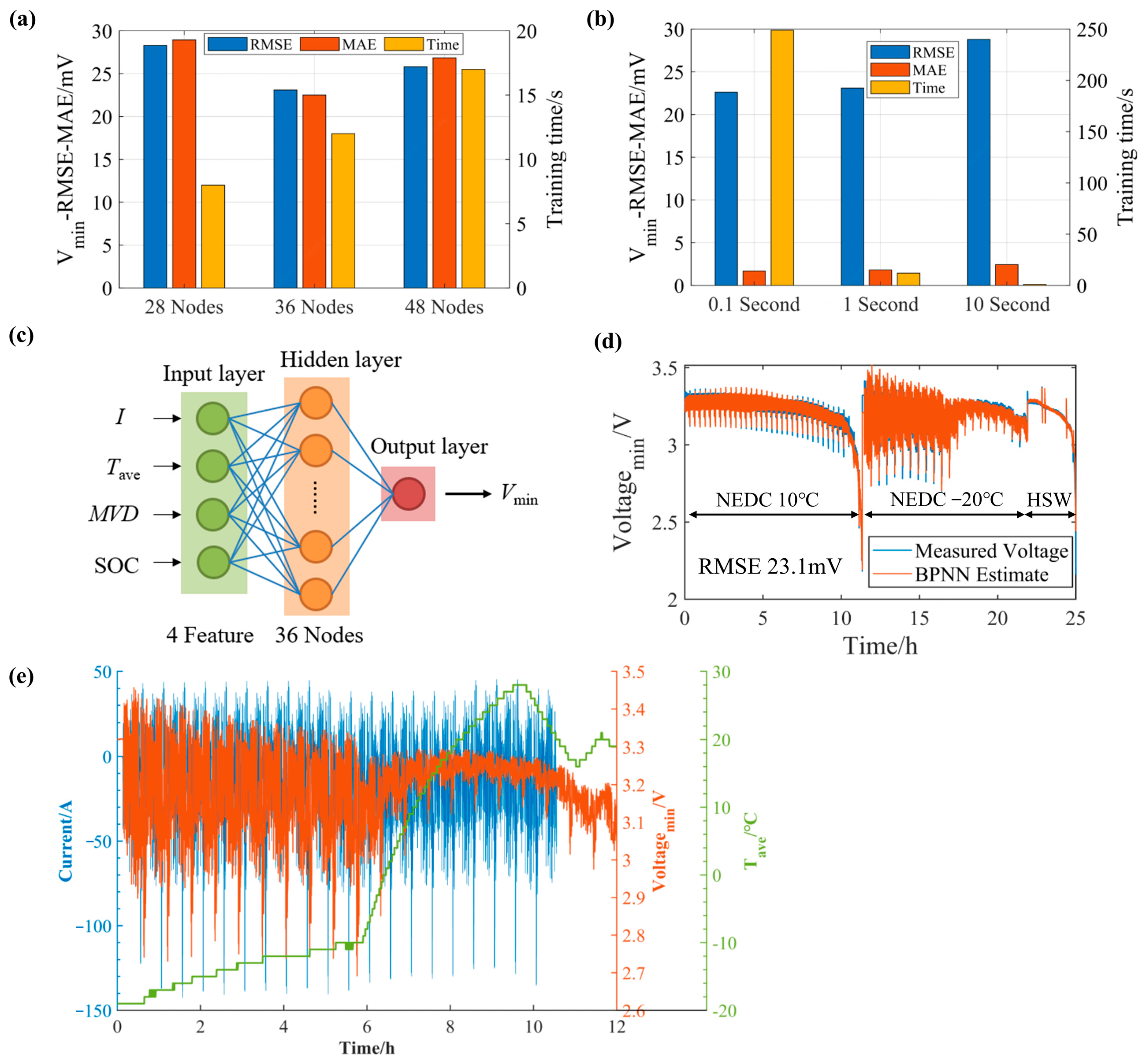
2.1. Training of the BPNN Model

BPNN is a widely used neural network model that maps non-linear relationships between input and output using activation functions, and updates node parameters in different layers using a backpropagation algorithm. The voltage characteristics of LiFePO₄ batteries change significantly at different temperatures, especially at low temperatures, where the internal polarization of the battery increases and voltage changes sharply. Traditional ECM often lacks accuracy. To accurately capture the complex relationship between SOC, current, temperature, and terminal voltage, the LiFePO₄ battery system is tested under −25 °C to 43 °C using the New European Driving Cycle (NEDC) and high-speed working (HSW) conditions to construct a neural network training dataset. The minimum terminal voltage of the battery system is used as the output target, and feature selection is performed using the Pearson correlation coefficient (PCC). The simulation accuracy of the BPNN test set is evaluated under different hyperparameters to determine the optimal neural network structure.

2.1.1. Dataset Construction

The typical parameters of the blade LiFePO₄ battery are shown in

Table 1. Typical parameters of the LiFePO₄ blade battery cell.

Battery Cell	Specification
Cathode material	LiFePO4
Anode material	Graphite
Nominal capacity	135 Ah
Nominal voltage	3.2 V
Charging cutoff voltage	3.8 V
Discharging cutoff voltage	2.0 V

and

Table 2. Typical parameters of the LiFePO₄ blade battery system.

Battery System	Specification
Configuration	178S1P
Nominal voltage	570 V
Nominal capacity	135 Ah
Nominal energy capacity	76.9 kWh

. The battery cell is rectangular, with LiFePO₄ as the positive electrode material and graphite as the negative electrode. The rated capacity is 135 Ah, the charge cut-off voltage is 3.8 V, and the discharge cut-off voltage is 2.0 V. The blade battery system consists of a 178S1P configuration with a rated voltage of 570 V and a system energy of 76.9 kWh. This battery pack is installed in the BYD Auto Industry Company Limited Han electric vehicle.

As shown in Figure 1, the experiment is conducted on a blade battery system and divided into laboratory and field tests. The laboratory test placed the battery system in a programmable temperature box, simulated working conditions using a charge-discharge machine to input current excitation, and collected voltage and temperature signals. The sampling time is 0.1 s, and the voltage sampling system contains the highest and lowest voltage of the battery system’s single cells with a voltage sampling resolution of 0.001 mV and a current sampling resolution of 0.001 mA. Multiple temperature sampling points are distributed throughout the battery system, and the temperature monitoring system provides the system’s average temperature, and the highest and lowest temperatures recorded, with a temperature sampling resolution of 1 °C. Before testing, the battery system is fully charged at 25 °C.

To obtain battery characteristics at different temperatures, NEDC working condition tests are conducted at −25 °C, −20 °C, −5 °C, 0 °C, 10 °C, 25 °C, and 45 °C. For field tests, the driver simulates the NEDC working conditions during on-road driving tests conducted at −7 °C and −20 °C. In addition, field driving tests are performed on a Chinese highway at a speed of 120 km/h, with testing ambient temperatures of 35 °C and 30 °C, namely 35 °C HSW and 30 °C HSW. During the field driving tests, time, voltage, current, and temperature signals are sampled using an onboard sampling chip with the same sampling time and accuracy as in the laboratory. Therefore, this experiment data set consists of eleven working condition tests, seven laboratory tests, and four field driving tests.

To train the BPNN model, the above working conditions need to be divided into training, validation, and testing sets. The division of the experimental data set is shown in Figure 2. In this research, the −25 °C NEDC, −5 °C NEDC, 0 °C NEDC, 25 °C NEDC, 43 °C NEDC, and 30 °C HSW are assigned to the training set, and the field tests of −20 °C NEDC and −7 °C NEDC are assigned to the validation set. The testing set includes 10 °C NEDC, −20 °C NEDC, and 35 °C HSW working conditions. The testing set includes three working conditions: a low-temperature condition of −20 °C to verify the model’s applicability in low-temperature environments, and 10 °C NEDC and 35 °C HSW working conditions to test the model’s accuracy under different working conditions and temperatures.

2.1.2. Feature Selection

After constructing the dataset, it is necessary to determine the input features and output targets of the BPNN model. As this study aims to estimate the SOC of the entire battery system during the discharge process, the main focus is on the minimum discharge voltage of the series-connected battery system. The target output of the BPNN is the minimum discharge voltage of the battery system. In terms of input features, the initial selection included maximum voltage difference (MVD), maximum temperature difference (MTD), current (I), average temperature (T_ave), current change rate (CCR), average temperature change rate (ATCR), and SOC as input features. A detailed description of the selected features is shown in

Table 3. Neural network feature meanings.

Feature Name	Description
Maximum voltage difference (MVD)	The difference between the highest and lowest voltage of individual cells within the series-connected blade battery system.
Maximum temperature difference (MTD)	The difference between the highest temperature sampling data and the lowest temperature sampling data within the series-connected blade battery pack.
Current (I)	The current flowing through the series-connected blade battery pack, with positive value indicating charging.
Average temperature (Tave)	The average value of temperature sampling data within the series-connected blade battery pack.
Current change rate (CCR)	The difference in current between two sampling intervals.
Average temperature change rate (ATCR)	The difference in average temperature between two sampling intervals.
State of charge (SOC)	The available capacity of the battery divided by its nominal capacity (135 Ah).

.

To explore the relationship between input features and output voltage, PCC is used to screen the main features. PCC is a way to measure the correlation between input and output features, with an output range from −1 to +1, where 0 represents no correlation, negative values represent negative correlation, and positive values represent positive correlation. The calculation of the PCC is shown in Equations (1)–(3), and the results are shown in Figure 3. The correlation coefficient between the same features is 1, and if two different features are positively correlated, they are represented by light green, while negative correlation is represented by white. Based on the results of the PCC, the four features with the highest absolute correlation are selected as input features of the BPNN, including MVD, I, SOC, and T_ave, which are found to be most relevant to the output. The PCC for these four features is highlighted in red in Figure 3.

$$r_f=\frac{{\sum }_{i=1}^k(f_i-\overline{f})(v_{\mathrm{m}\mathrm{i}\mathrm{n},i}-\overline{v_{\mathrm{m}\mathrm{i}\mathrm{n}}})}{\sqrt{{\sum }_{i=1}^k{(f_i-\overline{f})}^2}\sqrt{{\sum }_{i=1}^k{(v_{\mathrm{m}\mathrm{i}\mathrm{n},i}-\overline{v_{\mathrm{m}\mathrm{i}\mathrm{n}}})}^2}}$$

(1)

$$\overline{f}=\frac{1}{k}{\sum }_{i=1}^k{f}_i$$

(2)

$$\overline{v_{\mathrm{m}\mathrm{i}\mathrm{n}}}=\frac{1}{k}{\sum }_{i=1}^k{v}_{\mathrm{m}\mathrm{i}\mathrm{n}}$$

(3)

where $r_f$ represents the PCC between the input features and the output, and $f_i$ and $v_{\mathrm{m}\mathrm{i}\mathrm{n},i}$ are the feature variable value and the minimum voltage of the battery system at index sequence $i$ in the dataset, respectively. $\overline{f}$ and $\overline{v_{\mathrm{m}\mathrm{i}\mathrm{n}}}$ are the mean value, and $k$ is the length of the dataset.

2.1.3. BPNN Training

The network structure of the BPNN model mainly consists of an input layer, a hidden layer, and an output layer. After feature selection, the input layer selected four features, including MVD, I, SOC, and T_ave, and the output layer’s output value is the minimum terminal voltage of the battery system. The structure of the hidden layer also needs to be determined.

To reduce the complexity of the entire model, a single hidden layer is chosen. The nonlinear activation function of the BPNN is the hyperbolic tangent function, as shown in Equation (4). The Levenberg–Marquardt algorithm is adopted for the training algorithm. The Levenberg–Marquardt algorithm is a variation of Newton’s method, used to minimize the sum of squares of the nonlinear loss function in a BPNN model. The core idea is to use the Jacobian matrix (which is easier to compute) as a replacement for the computation of the Hessian matrix, thereby improving the efficiency of optimization. The Levenberg–Marquardt algorithm is a standard numerical optimization method that accelerates the training of BPNN model.

$$\mathrm{tansig}\left(x\right)=\frac{\sinh (x)}{\cosh (x)}=\frac{e^x-e^{-x}}{e^x+e^{-x}}$$

(4)

where $\mathrm{tansig}$ is the hyperbolic tangent function, $\sinh$ is the hyperbolic sine function, $\cosh$ is the hyperbolic cosine function, e is the Euler number.

To ensure the generalization of the BPNN model, the training ends when the training error on the validation set does not decrease for six consecutive times. Before model training, feature normalization is required to eliminate the influence of differences in units and scales between features, and each feature is treated equally. The normalization calculation formula is shown in Equation (5). The mathematical expression of the neural network is shown in Equation (6).

$$z=\frac{{(z}_{\mathrm{m}\mathrm{a}\mathrm{x}}-z_{\mathrm{m}\mathrm{i}\mathrm{n}})(p-p_{\mathrm{m}\mathrm{i}\mathrm{n}})}{p_{\mathrm{m}\mathrm{a}\mathrm{x}}-p_{\mathrm{m}\mathrm{i}\mathrm{n}}}+z_{\mathrm{m}\mathrm{i}\mathrm{n}}$$

(5)

where $z$ is the normalized value of the feature, $p_{\mathrm{m}\mathrm{a}\mathrm{x}}$ and $p_{\mathrm{m}\mathrm{i}\mathrm{n}}$ are the upper and lower limits of the normalization interval, respectively, which are +1 and −1, $z_{\mathrm{m}\mathrm{a}\mathrm{x}}$ is the maximum value of the feature, and $z_{\mathrm{m}\mathrm{i}\mathrm{n}}$ is the minimum value of the feature.

$$v_{min}=W_2\times \mathrm{t}\mathrm{a}\mathrm{n}\mathrm{s}\mathrm{i}\mathrm{g}\left(W_1\times z+b_1\right)+b_2$$

(6)

where $v_{min}$ represents the neural network output, $z$ represents the input feature vector, $W_1$ and $W_2$ are the weight matrices between the input layer and the hidden layer, and between the hidden layer and the output layer, respectively. $b_1$ and $b_2$ are bias vectors, and tansig is the nonlinear activation function used in the hidden and output layers.

To explore the optimal number of nodes in the hidden layer, single-hidden-layer BPNN models with 28, 36, and 48 nodes are trained, and the simulation errors of the test set and training time are compared for different node numbers. Matlab R2020b, the computational platform used for BPNN training, is run on the Intel (R) Xeon (R) Gold 62486R CPU @ 3.00 Ghz @ 2.99 Ghz (two processors) with 16 GB RAM. As shown in Figure 4a, with the increase in the number of nodes, the model training time increases, but the root mean square error (RMSE) and mean absolute error (MAE) of the model on the test set do not decrease. Increasing the number of nodes brings difficulties to the model training. A total of 36 nodes are chosen as the optimal number of nodes in the hidden layer. The actual data sampling time is 0.1 s. When training the neural network model with 0.1 s sampling data, the training time is 249 s, voltage simulation RMSE is 22.6 mV, and MAE is 14.1 mV. When training the BPNN model with 1 s interval sampling data, the training time can be significantly reduced to 12 s, 4.8% of the original training time. The RMSE and MAE of the terminal voltage simulation only increased by 2.21% and 6.38%, respectively. When selecting data with a 10 s interval for training the model, the terminal voltage simulation error increases significantly, with RMSE increasing to 28.8 mV and MAE to 20.4 mV. Considering the trade-off between model training time cost and accuracy, 1 s sampling data is chosen for model training. The final neural network model is shown in Figure 4c.

The performance of the BPNN model on the test set is shown in Figure 4d. The BPNN model shows good voltage simulation accuracy for the 10 °C NEDC, −20 °C NEDC, and 35 °C HSW working conditions, with an overall RMSE of 23.1 mV. It is worth noting that at −20 °C, the voltage fluctuation is severe in the initial stage, as shown in Figure 4e. This is due to the higher internal resistance of the battery at low temperatures, which results in a higher polarization voltage. After a certain amount of charge and discharge, the heat generated by the battery’s internal resistance increases the temperature, reducing the resistance value and narrowing the voltage fluctuation range. Under these conditions, with apparent changes in internal resistance, the BPNN model can still follow the voltage change trend very well, verifying the accuracy of the BPNN model.

2.2. BPNN-EKF Algorithm

The fundamental value for battery system SOC estimation is obtained through ampere-hour integration, as shown in Equation (7). However, since ampere-hour integration is an open-loop calculation method, it is susceptible to various noises, thus requiring calibration during real-world applications. Based on the BPNN voltage model, this research calibrates the SOC value obtained from the ampere-hour integration calculation using voltage error information. The calibration algorithm adopts the EKF algorithm, which can achieve optimal estimation in the least squares sense. Firstly, a state equation is established for the battery system, and EKF iterative calculation is performed. The input vector of the state equation is the current value, the state vector is the SOC value, and the observation value is the minimum voltage of the battery system. The transition matrices in the state Equation (11) are shown respectively in Equations (12) and (13). The key to the BPNN-EKF fusion is to determine the expression of the Kalman gain, which is obtained by taking the derivative of the SOC concerning the output voltage value from the BPNN model. The derivative result is shown in Equations (14) and (15), and mathematical operations are performed using the trained neural network model matrix. This Kalman gain term avoids the traditional OCV differentiation with respect to SOC in the ECM model, and can achieve a more stable calibration effect for SOC. The BPNN-EKF algorithm framework is shown in Figure 5. The covariance matrix P takes a value of 1, Q takes a value of 10⁻⁹, and R takes a value of 0.5.

$${\mathrm{S}\mathrm{O}\mathrm{C}}_t={\mathrm{S}\mathrm{O}\mathrm{C}}_0+{\int }_{t_0}^t\frac{\eta I}{Q_{system}}d\tau$$

(7)

where ${\mathrm{S}\mathrm{O}\mathrm{C}}_t$ represents the SOC value at time $t$, ${\mathrm{S}\mathrm{O}\mathrm{C}}_0$ is the initial value of SOC, $t_0$ is the initial calculation time, $\eta$ is the Coulomb efficiency with a value of 1, $I$ is the current value, positive for charging and negative for discharging, and $Q_{system}$ is the battery system capacity with a nominal value of 135 Ah.

$$u_t=I_t$$

(8)

$$x_t={\mathrm{S}\mathrm{O}\mathrm{C}}_t$$

(9)

$$y_t=V_{\mathrm{m}\mathrm{i}\mathrm{n},t}+{\nu }_t$$

(10)

$$x_t={Ax}_{t-1}+{Bu}_{t-1}+{\omega }_{t-1}$$

(11)

$$A=1$$

(12)

$$B=-\frac{∆t}{3600\times Q_{system}}$$

(13)

$${H_t}_t=\frac{{\mathit{\partial }V}_{min}}{\mathit{\partial }{x}_t}=W_2\times (W_1\times {\left[\mathrm{0,0},\mathrm{1,0}\right]}^{\mathrm{T}})\times ({\left[1;\dots ;1\right]}_{36\times 1}-\mathrm{t}\mathrm{a}\mathrm{n}\mathrm{s}\mathrm{i}\mathrm{g}{(b_1)}^2)$$

(14)

$$K_t=P_t^{-}{H}_t^T{(H_t{P}_t^{-}{H}_t^T+R)}^{-1}$$

(15)

where $u_t$ represents the input variable, $x_t$ represents the state variable, and $y_t$ represents the observed variable. $A$ and $B$ are state transition matrices, and $\omega$ represents the model noise, while $\nu$ represents the observation noise. It is assumed that both $\omega$ and $\nu$ variables follow a Gaussian distribution, $H_t$ is the Jacobian matrix, $K_t$ is the Kalman gain, $P_t^{-}$ and $R$ are covariance matrix.

In this section, NEDC and HSW tests are conducted on a series-connected battery pack of LiFePO₄ blade batteries under different temperatures in both laboratory and field scenarios. The test results are divided into training, validation, and testing sets to train a BPNN model with the minimum terminal voltage as the output. By calculating the PCC between different physical features and the minimum terminal voltage of the series-connected battery system, the most correlated features, namely MVD, I, SOC and T_ave, are selected as input features for the BPNN. By comparing the training results, the number of nodes in the hidden layer of the neural network is determined to be 36, and the sampling interval for training the network is set to 1 s. The constructed neural network model achieved a low RMSE of only 23.6 mV in simulating the terminal voltage under −20 °C NEDC, 10 °C NEDC, and 35 °C HSW validation working conditions, indicating high simulation accuracy. Furthermore, the expression for the Kalman gain, which integrates the output terminal voltage of the BPNN, is derived and used for deep fusion with the EKF algorithm. The BPNN-EKF algorithm utilizes the error between simulated voltage and measured voltage to correct the initial value of SOC based on ampere-hour integration. The algorithm is not only applicable to the LiFePO₄ battery system but also suitable for nickel-cobalt-manganese (NCM) lithium ion batteries and lithium manganese iron phosphate batteries. It only requires training the BPNN model with experimental data from different battery systems. The fusion of EKF and BPNN models remains the same. However, considering the limited types of test conditions currently available, to apply this algorithm in the real world, it is necessary to increase the amount of training data in the training set to improve the model’s universality.

3. SOC Estimation Results

3.1. Ideal Situation

The SOC estimation algorithm is validated on test conditions of −20 °C NEDC, 10 °C NEDC, and 35 °C HSW, with SOC reference values obtained by accurate initial SOC values and ampere-hour integration. The SOC estimation results for the three test working conditions without considering other errors are shown in Figure 6a–c, with RMSE errors of 1.81%, 2.26%, and 1.36%, respectively. The BPNN-EKF algorithm has a SOC estimation error of less than 2% in the −20 °C low-temperature and has desirable estimation results in the 10 °C NEDC and 35 °C HSW, demonstrating the effectiveness of the algorithm for wide temperature range and different working conditions SOC estimation. The absolute error of SOC exhibited a fluctuating pattern, with the EKF algorithm correcting the SOC error.

3.2. Algorithm Robustness Verification

In practical situations, the performance of a battery system is affected by various sources of noise and interference, and real-time computation is required for onboard applications. To better fit real-world scenarios, the capacity of a battery may have errors, the sampling of current and voltage may have random noise, and the initial SOC may have errors. Moreover, the SOC calculation intervals also affect the accuracy of SOC estimation. Therefore, evaluating the robustness and accuracy of the SOC estimation algorithm under different scenarios is necessary.

3.2.1. Capacity Error

During the use of electric vehicle batteries, their capacity gradually decays; therefore, the battery capacity needs to be estimated. However, capacity estimation is subject to errors. The error in capacity directly affects the accuracy of SOC estimation. When there is a negative bias in capacity, SOC estimation methods based on ampere-hour integration can result in an overestimation of SOC, and this bias persists over time. This can potentially lead to over-discharging of the battery, posing safety risks. Overestimated SOC values can cause voltage discrepancies between model predictions and actual measurements during the discharge process. The BPNN-EKF algorithm can be employed to correct the SOC based on this voltage error information.

This research evaluates the accuracy of SOC estimation using the BPNN-EKF algorithm under the assumption of a 5% capacity negative error. The results of SOC estimation under test working conditions of −20 °C NEDC, 10 °C NEDC, and 35 °C HSW are presented in Figure 6d–f, with RMSE of 3.98%, 2.16%, and 1.37%, respectively. Compared to the scenario without capacity error, the errors are virtually unchanged at 10 °C NEDC and 35 °C HSW, and increased by only 2% at −20 °C NEDC, indicating that the BPNN-EKF algorithm is robust to the errors caused by capacity estimation in these three working conditions. The fact that the RMSE of SOC remains essentially unchanged implies that the BPNN-EKF algorithm is not significantly affected by capacity errors.

3.2.2. Current and Voltage Sampling Error

The current and voltage sampling devices have a certain sampling accuracy, and produce random noise during sampling. The noise in current sampling also affects the SOC calculation method based on ampere-hour integration in the BPNN-EKF algorithm, while voltage sampling errors introduce disturbances to the model-based SOC feedback correction algorithm. The robustness and accuracy of the BPNN-EKF algorithm in this scenario need further validation.

To verify the accuracy and robustness of the BPNN-EKF algorithm in SOC estimation under current and voltage sampling errors, we introduced a random noise of −10% to +10% to the original voltage sampling data and a random noise of −20% to +20% to the original current sampling data. The process of applying current and voltage noise to the original data is illustrated in Figure 7. Figure 7a depicts the flowchart of the random noise injection process. Figure 7b shows the random noise added to the original voltage sampling data. Figure 7c compares the original voltage sampling data with the voltage noise data. Figure 7d displays the random noise added to the original current sampling data. Lastly, Figure 7e compares the original current sampling data with the current noise data. The SOC estimation algorithm is validated under the combined effect of current and voltage sampling errors, and the SOC estimation results are shown in Figure 6g–i. The SOC estimation RMSE is 1.54% under the −20 °C NEDC working condition, 2.51% under the 10 °C NEDC working condition, and 1.55% under the 35 °C HSW working condition. Even with the superimposed sampling errors, the SOC estimation can still maintain high accuracy, indicating that the BPNN-EKF algorithm is not sensitive to sampling noise because voltage error information is the core source of SOC correction, and random voltage noise can increase error information and enhance the correction effect of SOC. The SOC estimation accuracy of the BPNN-EKF algorithm can still be maintained at a high level even when there are sampling errors in voltage and current.

3.2.3. Initial SOC Error

In practical situations, the initial SOC value may not be accurate. Correcting the initial SOC during operation helps drivers obtain accurate battery state information, and enables them to engage in appropriate driving behavior. The initial SOC error also generates voltage error information, which can be captured by BPNN-EKF to correct the initial SOC error.

A simulation scenario with a relatively severe 20% initial error is set up to verify the algorithm’s estimation accuracy. The simulation results of SOC are shown in Figure 8a,d,g. The RMSE errors are 1.81%, 3.62%, and 1.52% under −20 °C NEDC, 10 °C NEDC, and 35 °C HSW, respectively. The process of correcting the initial SOC error gradually reduces the SOC error. If the correction is done too quickly, the RMSE of SOC estimation remains essentially unchanged, for example, under the −20 °C NEDC working condition. If the correction speed is slightly slower, it can increase the RMSE of SOC estimation, for example, under the 10 °C NEDC and 35 °C HSW working conditions. This indicates that the accuracy of the battery model is crucial in the early stages of operation. Due to the large initial SOC error, the voltage error information is significantly increased, thereby enhancing the SOC correction effect and making the SOC error quickly converge. The Kalman gain curve and its early amplification are shown in Figure 8b,c,e,f,h,i. The equation shown in Equation (16) represents the correction of the SOC feedforward value using the Kalman gain and voltage error. When the SOC error is large, the voltage error increases. With the assistance of a stable Kalman gain, this leads to a larger correction effect, allowing the SOC to rapidly approach the true value. Under the −20 °C NEDC working condition, with a 20% initial error in the early stage, the Kalman gain rapidly increased to about 0.6, forming a strong SOC correction effect, making the quick SOC approach the true value. Under 10 °C NEDC and 35 °C HSW working conditions, the Kalman gain is also large and showed a fluctuating feature and the absolute SOC error continued to decrease.

$$x_t^{+}=x_t^{-}+K_t(y_t-v_{\mathrm{m}\mathrm{i}\mathrm{n}})$$

(16)

where $x_t^{+}$ represents the SOC after correction by the EKF algorithm, $x_t^{-}$ represents the SOC calculated through ampere-hour integration method, $K_t$ represents the Kalman gain, $y_t$ represents the measured minimum voltage value in the series-connected battery pack, and $v_{\mathrm{m}\mathrm{i}\mathrm{n}}$ represents the predicted minimum voltage value in the series-connected battery pack by the BPNN model.

3.2.4. Interval Calculation of SOC

Considering the limitation of computing power in actual vehicles, calculating SOC every 1 s may burden the BMS management system significantly. When the hardware of the battery management system is constrained by computational power, it may be necessary to calculate SOC at intervals of multiple seconds. Within adjacent calculation intervals, the SOC value remains constant and cannot reflect the true SOC value. However, the voltage error caused by SOC errors also generates a Kalman gain, which can be used to correct it through the BPNN-EKF algorithm. We utilize this scenario to further validate the robustness of the BPNN-EKF algorithm.

The SOC estimation results at intervals of 5 s, 10 s, and 30 s are shown in Figure 9. As the calculation time interval increases, the SOC estimation error increases, and the error fluctuation shows an increasing trend because the calculated SOC value does not change during the interval, causing the difference between the calculated SOC and the accurate SOC to increase. When the calculation is resumed, the continuous SOC difference brings voltage error information, corrected by the EKF algorithm, and the SOC error is further reduced. Therefore, the absolute SOC error fluctuates continuously. Overall, the SOC still has good accuracy and robustness at different calculation time intervals. Under a 30 s interval, the BPNN-EKF algorithm has an RMSE error of 3.04% at −20 °C NEDC, 2.85% at 10 °C NEDC, and 1.68% at 35 °C HSW working conditions.

As shown in the Figure 10, the BPNN-EKF algorithm demonstrated high accuracy in estimating SOC under four different scenarios: capacity error, errors in current and voltage sampling, error in initial SOC, and interval SOC calculation. The algorithm showed good resistance to various errors attributed to the fusion of the Kalman gain calculation and the output voltage of the BPNN. The stability of SOC estimation is improved by using voltage information to correct SOC errors. The algorithm is suitable for various operating conditions. Under the low-temperature NEDC working condition of −20 °C, the BPNN model can track the tremendous nonlinear changes in voltage well, and the maximum SOC estimation error is 3.98%. Under the 10 °C NEDC working condition, the maximum RMSE of SOC estimation is 3.62%; under the 35 °C HSW working condition, the maximum RMSE of SOC estimation is 1.49%. The BPNN-EKF algorithm, with its strong robustness and high accuracy, holds great potential for application in real-world electric vehicle management systems. It can significantly enhance the precision of SOC estimation in battery systems, enabling drivers to have a better awareness of the battery’s state. By improving SOC estimation accuracy, potential safety risks can be effectively mitigated. This algorithm has the capability to contribute to the overall safety and performance of electric vehicles, providing reliable information about the battery’s status for optimal driving and preventing any potential safety hazards.

4. Conclusions

The LiFePO₄ batteries, known for their flat open-circuit voltage and significant polarization at different temperatures, pose challenges in accurately modeling their voltage behavior. This difficulty in voltage modeling presents a challenge for model-based SOC estimation algorithms. Additionally, the current state of SOC estimation algorithms shows poor robustness and accuracy under different operating conditions and temperatures, further contributing to potential safety risks in electric vehicles. This research focuses on the LiFePO₄ blade battery system and proposes a BPNN-EKF algorithm for accurate SOC estimation, which addresses the inaccurate voltage model simulation issues under a wide temperature range, approximate SOC estimation at low temperatures, and the insufficient robustness in the SOC estimation algorithm for LiFePO₄ batteries.

The main contributions are summarized as follows:

(1) A BPNN model is constructed to simulate the minimum terminal voltage of the blade battery system with high accuracy under a wide temperature range (25–43 °C) through feature selection and hyperparameter tuning. The maximum RMSE of the terminal voltage under −20 °C NEDC, 10 °C NEDC, and 35 °C HSW test working conditions is only 23.1 mV. An accurate voltage model can generate stable voltage error information in the presence of SOC errors, thereby correcting SOC estimation errors. This is particularly crucial in blade battery systems, where our developed BPNN-EKF algorithm utilizes voltage to differentiate SOC. As a result, an accurate voltage model will generate stable Kalman gains, enhancing the robustness and accuracy of SOC estimation.

(2) Based on the BPNN model for terminal voltage output, we derive the expression for calculating the Kalman gain and achieve deep fusion of BPNN and EKF algorithms. We then utilize the BPNN-EKF algorithm to accurately estimate the blade battery system’s SOC. The BPNN-EKF algorithm demonstrated high SOC simulation accuracy under different scenarios, with low capacity, current, voltage sampling, initial SOC, and interval SOC calculation errors. The maximum SOC estimation RMSE is 3.98% at −20 °C NEDC, 3.62% at 10 °C NEDC, and 1.68% at 35 °C HSW. The BPNN-EKF algorithm has the potential to be applied in BMS to achieve high accuracy and robustness in SOC estimation, especially under wide temperature ranges and various operating conditions. This method aims to provide more accurate battery status information to drivers, resulting in an improved driving experience and mitigating potential safety risks.

The BPNN-EKF SOC estimation algorithm is not only applicable to LiFePO₄ batteries but also exhibits its versatility to be applied to batteries of other chemistries. The accuracy of SOC estimation across different battery systems is worth further validation in the future. Additionally, the consideration of NEDC and HSW operating conditions alone is insufficient. To enhance the accuracy of the BPNN model, it is necessary to incorporate a broader range of real-world operating conditions during model training to improve its applicability.

References

1. Li, Y.; Wei, Y.; Zhu, F.; Du, J.; Zhao, Z.; Ouyang, M. The path enabling storage of renewable energy toward carbon neutralization in China. Etransportation 2023, 16, 100226. [Google Scholar] [CrossRef]
2. Dixon, J.; Bukhsh, W.; Bell, K.; Brand, C. Vehicle to grid: Driver plug-in patterns, their impact on the cost and carbon of charging, and implications for system flexibility. Etransportation 2022, 13, 100180. [Google Scholar] [CrossRef]
3. Hu, G.; Huang, P.; Bai, Z.; Wang, Q.; Qi, K. Comprehensively analysis the failure evolution and safety evaluation of automotive lithium ion battery. Etransportation 2021, 10, 100140. [Google Scholar] [CrossRef]
4. Wang, X.; Wei, X.; Zhu, J.; Dai, H.; Zheng, Y.; Xu, X.; Chen, Q. A review of modeling, acquisition, and application of lithium-ion battery impedance for onboard battery management. Etransportation 2021, 7, 100093. [Google Scholar] [CrossRef]
5. Liu, Y.; Zhang, C.; Jiang, J.; Zhang, L.; Zhang, W.; Wang, L.Y. Deduction of the transformation regulation on voltage curve for lithium-ion batteries and its application in parameters estimation. Etransportation 2022, 12, 100164. [Google Scholar] [CrossRef]
6. Liu, W.; Hu, X.; Lin, X.; Yang, X.-G.; Song, Z.; Foley, A.M.; Couture, J. Toward high-accuracy and high-efficiency battery electrothermal modeling: A general approach to tackling modeling errors. Etransportation 2022, 14, 100195. [Google Scholar] [CrossRef]
7. Mao, S.; Han, M.; Han, X.; Lu, L.; Feng, X.; Su, A.; Wang, D.; Chen, Z.; Lu, Y.; Ouyang, M. An Electrical–Thermal Coupling Model with Artificial Intelligence for State of Charge and Residual Available Energy Co-Estimation of LiFePO4 Battery System under Various Temperatures. Batteries 2022, 8, 140. [Google Scholar] [CrossRef]
8. Song, Z.; Yang, X.-G.; Yang, N.; Delgado, F.P.; Hofmann, H.; Sun, J. A study of cell-to-cell variation of capacity in parallel-connected lithium-ion battery cells. Etransportation 2021, 7, 100091. [Google Scholar] [CrossRef]
9. Liu, Z.; Li, Z.; Zhang, J.; Su, L.; Ge, H. Accurate and efficient estimation of lithium-ion battery state of charge with alternate adaptive extended Kalman filter and ampere-hour counting methods. Energies 2019, 12, 757. [Google Scholar] [CrossRef] [Green Version]
10. Xiong, X.; Wang, S.L.; Fernandez, C.; Yu, C.M.; Zou, C.Y.; Jiang, C. A novel practical state of charge estimation method: An adaptive improved ampere-hour method based on composite correction factor. Int. J. Energy Res. 2020, 44, 11385–11404. [Google Scholar] [CrossRef]
11. Xiao, T.; Shi, X.; Zhou, B.; Wang, X. Comparative Study of EKF and UKF for SOC Estimation of Lithium-ion Batteries. In Proceedings of the 2019 IEEE Innovative Smart Grid Technologies-Asia (ISGT Asia), Chengdu, China, 21–24 May 2019; pp. 1570–1575. [Google Scholar]
12. Yu, Q.; Huang, Y.; Tang, A.; Wang, C.; Shen, W. OCV-SOC-Temperature Relationship Construction and State of Charge Estimation for a Series–Parallel Lithium-Ion Battery Pack. IEEE Trans. Intell. Transp. Syst. 2023, 24, 6362–6371. [Google Scholar] [CrossRef]
13. Fan, K.; Wan, Y.; Wang, Z.; Jiang, K. Time-efficient identification of lithium-ion battery temperature-dependent OCV-SOC curve using multi-output Gaussian process. Energy 2023, 268, 126724. [Google Scholar] [CrossRef]
14. Dreyer, W.; Jamnik, J.; Guhlke, C.; Huth, R.; Moškon, J.; Gaberšček, M. The thermodynamic origin of hysteresis in insertion batteries. Nat. Mater. 2010, 9, 448–453. [Google Scholar] [CrossRef]
15. Hu, X.; Li, S.; Peng, H. A comparative study of equivalent circuit models for Li-ion batteries. J. Power Sources 2012, 198, 359–367. [Google Scholar] [CrossRef]
16. Doyle, M.; Fuller, T.F.; Newman, J. Modeling of galvanostatic charge and discharge of the lithium/polymer/insertion cell. J. Electrochem. Soc. 1993, 140, 1526. [Google Scholar] [CrossRef]
17. Han, X.; Ouyang, M.; Lu, L.; Li, J. Simplification of physics-based electrochemical model for lithium ion battery on electric vehicle. Part I: Diffusion simplification and single particle model. J. Power Sources 2015, 278, 802–813. [Google Scholar] [CrossRef]
18. Hu, X.; Feng, F.; Liu, K.; Zhang, L.; Xie, J.; Liu, B. State estimation for advanced battery management: Key challenges and future trends. Renew. Sustain. Energy Rev. 2019, 114, 109334. [Google Scholar] [CrossRef]
19. Wang, Y.; Tian, J.; Sun, Z.; Wang, L.; Xu, R.; Li, M.; Chen, Z. A comprehensive review of battery modeling and state estimation approaches for advanced battery management systems. Renew. Sustain. Energy Rev. 2020, 131, 110015. [Google Scholar] [CrossRef]
20. Plett, G.L. Extended Kalman filtering for battery management systems of LiPB-based HEV battery packs: Part 3. State and parameter estimation. J. Power Sources 2004, 134, 277–292. [Google Scholar] [CrossRef]
21. Wang, L.; Han, J.; Liu, C.; Li, G. State of charge estimation of lithium-ion based on VFFRLS-noise adaptive CKF algorithm. Ind. Eng. Chem. Res. 2022, 61, 7489–7503. [Google Scholar] [CrossRef]
22. Anton, J.C.A.; Nieto, P.J.G.; Gonzalo, E.G.; Pérez, J.C.V.; Vega, M.G.; Viejo, C.B. A new predictive model for the state-of-charge of a high-power lithium-ion cell based on a PSO-optimized multivariate adaptive regression spline approach. IEEE Trans. Veh. Technol. 2015, 65, 4197–4208. [Google Scholar] [CrossRef]
23. Yao, J.; Ding, J.; Cheng, Y.; Feng, L. Sliding mode-based H-infinity filter for SOC estimation of lithium-ion batteries. Ionics 2021, 27, 5147–5157. [Google Scholar] [CrossRef]
24. How, D.N.T.; Hannan, M.A.; Lipu, M.S.H.; Ker, P.J. State of charge estimation for lithium-ion batteries using model-based and data-driven methods: A review. IEEE Access 2019, 7, 136116–136136. [Google Scholar] [CrossRef]
25. Fu, B.; Wang, W.; Li, Y.; Peng, Q. An improved neural network model for battery smarter state-of-charge estimation of energy-transportation system. Green Energy Intell. Transp. 2023, 2, 100067. [Google Scholar] [CrossRef]
26. Chen, J.; Zhang, Y.; Wu, J.; Cheng, W.; Zhu, Q. SOC estimation for lithium-ion battery using the LSTM-RNN with extended input and constrained output. Energy 2023, 262, 125375. [Google Scholar] [CrossRef]
27. Ren, Z.; Du, C. A review of machine learning state-of-charge and state-of-health estimation algorithms for lithium-ion batteries. Energy Rep. 2023, 9, 2993–3021. [Google Scholar] [CrossRef]
28. Wang, W.; Ma, B.; Hua, X.; Zou, B.; Zhang, L.; Yu, H.; Yang, K.; Yang, S.; Liu, X. End-Cloud Collaboration Approach for State-of-Charge Estimation in Lithium Batteries Using CNN-LSTM and UKF. Batteries 2023, 9, 114. [Google Scholar] [CrossRef]
29. Kumar, C.; Zhu, R.; Buticchi, G.; Liserre, M. Sizing and SOC management of a smart-transformer-based energy storage system. IEEE Trans. Ind. Electron. 2017, 65, 6709–6718. [Google Scholar] [CrossRef]
30. Hong, J.; Wang, Z.; Chen, W.; Wang, L.-Y.; Qu, C. Online joint-prediction of multi-forward-step battery SOC using LSTM neural networks and multiple linear regression for real-world electric vehicles. J. Energy Storage 2020, 30, 101459. [Google Scholar] [CrossRef]
31. Jiao, M.; Wang, D.; Qiu, J. A GRU-RNN based momentum optimized algorithm for SOC estimation. J. Power Sources 2020, 459, 228051. [Google Scholar] [CrossRef]
32. Lopes, E.D.R.; Soudre, M.M.; Llanos, C.H.; Ayala, H.V.H. Nonlinear receding-horizon filter approximation with neural networks for fast state of charge estimation of lithium-ion batteries. J. Energy Storage 2023, 68, 107677. [Google Scholar] [CrossRef]
33. Srinivasan, V.; Newman, J. Existence of path-dependence in the LiFePO4 electrode. Electrochem. Solid-State Lett. 2006, 9, A110. [Google Scholar] [CrossRef]
Figure 1. Schematic diagram of battery experiments (a) 25 °C NEDC working condition; (b) 30 °C high-speed working condition; (c) the battery experimental platform; (d) on-vehicle data acquisition device; (e) the LiFePO4 blade battery cell; (f) series LiFePO4 blade battery system; (g) BYD Han electric vehicle.
Batteries 09 00333 g001
Figure 2. The experimental dataset and the current-voltage curves for different working conditions. The training set: (a) −25 °C NEDC, (b) −5 °C NEDC, (c) 0 °C NEDC, (d) 25 °C NEDC, (e) 43 °C NEDC, (f) 30 °C HSW. The validation set: (g) the field test of −20 °C NEDC (h) the field test of−7 °C NEDC. The testing set: (i) −20 °C NEDC, (j) 10 °C NEDC, (k) 35 °C HSW.
Batteries 09 00333 g002
Figure 3. Pearson correlation coefficient calculation results.
Batteries 09 00333 g003
Figure 4. BPNN training: (a) model training time and test set voltage RMSE under different hidden layer node numbers; (b) model training time and test set voltage RMSE error under 0.1 s, 1 s, and 10 s sampling data; (c) BPNN model architecture; (d) BPNN model training results on the test set; (e) voltage, current, and average temperature curves of −20 °C NEDC working condition.
Batteries 09 00333 g004
Figure 5. BPNN-EKF algorithm framework diagram.
Batteries 09 00333 g005
Figure 6. SOC estimation results. Ideal conditions: (a) −20 °C NEDC, (b) 10 °C NEDC, (c) 35 °C HSW. With 5% capacity error: (d) −20 °C NEDC, (e) 10 °C NEDC, (f) 35 °C HSW. Current and voltage sampling error: (g) −20 °C NEDC, (h) 10 °C NEDC, (i) 35 °C HSW.
Batteries 09 00333 g006
Figure 7. Process diagram for adding noise to current and voltage data. (a) the flowchart of the random noise injection process (b) the random noise added to the original voltage sampling data (c) the original voltage sampling data and the voltage noise data; (d) the random noise added to the original current sampling data, (e) the original current sampling data and the current noise data.
Batteries 09 00333 g007
Figure 8. SOC estimation results with an initial SOC error of 20%. −20 °C NEDC: (a) SOC estimation results, (b) Kalman gain, and (c) magnified view of the Kalman gain at the initial stage; 10 °C NEDC: (d) SOC estimation results, (e) Kalman gain, and (f) magnified view of the Kalman gain at the initial stage; 35 °C HSW: (g) SOC estimation results, (h) Kalman gain, and (i) magnified view of the Kalman gain at the initial stage.
Batteries 09 00333 g008
Figure 9. SOC estimation results with interval calculation. At 5 s: (a) −20 °C NEDC, (b) 10 °C NEDC, (c) 35 °C HSW; 10 s: (d) −20 °C NEDC, (e) 10 °C NEDC, (f) 35 °C HSW;30 s: (g) −20 °C NEDC, (h) 10 °C NEDC, (i) 35 °C HSW.
Batteries 09 00333 g009
Figure 10. SOC estimation results under ideal and different error conditions.
Batteries 09 00333 g010