Properties of Ion Complexes and Their Impact on Charge Transport in Organic Solvent-Based Electrolyte Solutions for Lithium Batteries: Insights from a Theoretical Perspective

Abstract

Electrolyte formulations in standard lithium ion and lithium metal batteries are complex mixtures of various components. In this article, we review molecular key principles of ion complexes in multicomponent electrolyte solutions in regards of their influence on charge transport mechanisms. We outline basic concepts for the description of ion–solvent and ion–ion interactions, which can be used to rationalize recent experimental and numerical findings concerning modern electrolyte formulations. Furthermore, we discuss benefits and drawbacks of empirical concepts in comparison to molecular theories of solution for a more refined understanding of ion behavior in organic solvents. The outcomes of our discussion provide a rational for beneficial properties of ions, solvent, co-solvent and additive molecules, and highlight possible routes for further improvement of novel electrolyte solutions.

1. Introduction

The use of multicomponent electrolyte solutions in modern electrochemical storage devices such as rechargeable lithium ion and lithium metal batteries (LIBs and LMBs) is of fundamental importance for effective ion shuttling and transport mechanisms [1,2,3,4,5,6,7,8,9,10]. Nowadays well-known fast charging rates as well as the impressive performance of recent LIB and LMB devices [11,12,13,14] are not possible without decades of intense research on advanced electrolyte compositions. Although often not known in detail, standard electrolyte formulations in commercial energy storage devices mostly include various organic solvents, a plethora of distinct lithium ion conducting salts, and a broad range of possible further components in order to fulfill several duties related to the performance and safety of the electrochemical cell [1,3,6]. In addition to ions and the main solvent, components with concentrations at the molar scale are usually called co-solvents, whereas all other species which have total mass ratios lower than 5 wt % are classified as additives [15]. It is worth noting that additives are most often used as flame retardants, for the formation of protective layers at the electrodes, or as ion solvation enhancers [15,16,17]. Prominent examples for standard electrolyte formulations are high dielectric constant solvents of cyclic alkyl carbonates such as propylene carbonate (PC) or ethylene carbonate (EC), which provide an enhanced dissolution of the lithium salts, in combination with linear esters such as dimethyl carbonate (DMC), or ethylmethyl carbonate (EMC) as co-solvents to decrease the viscosity of the solution [1,3,6,18,19]. In combination with one or more lithium ion conducting salts, it becomes clear that the underlying ion correlation and charge transport mechanisms in the solution reveal a high level of complexity. Despite important benefits in terms of relatively low cost, most components of liquid organic electrolyte formulations are highly flammable and their use is restricted to well-defined electrode voltage ranges [5,6,7,16]. Recent research thus focuses on novel electrolyte formulations with lower flammability, higher electrochemical and thermal stability, and the presence of multi-functional molecular groups in regards of improved efficiencies and safeties for next-generation LIBs, LMBs and dual ion batteries (DIBs) [1,3,6,7,8,16,18,20,21,22,23,24,25,26,27,28,29,30,31,32].

Whereas most electrolyte solutions are well characterized in terms of their thermophysical and electrochemical properties [1,3], less is known on the underlying molecular interactions between the components. Due to the complexity of the solution, previous theoretical approaches such as scaled particle theory [33] mostly focus on ad hoc molecular approximations, which are often too simple and not applicable for distinct species in non-ideal or non-homogeneous solutions [34]. Consequently, parts of the general research strategy for the development of improved electrolyte solutions rely on empirical concepts and simple rules of thumbs instead of a rigorous molecular understanding of interaction mechanisms. A prominent example is the often cited alchemical law similia similibus solvuntur, which means the same dissolves in the same. In regards of this approach, it is often assumed that polar solutes and specifically lithium salts are highly solvated by polar solvents, whereas they are nearly insoluble in apolar media. It is worth noting that broad discrepancies between the individual saturation concentrations for distinct lithium salts in various organic solvents highlight crucial limitations for this simple approach [8,28,30,35,36,37,38,39,40].

Hence, the development of novel electrolyte formulations often relies on limited molecular understanding, empirical arguments, theoretical approaches suffering from unspecific approximations, or previous experimental findings instead of a desirable frame-guided design of tailor-made components for distinct purposes. In this context, refined theoretical and numerical approaches often provide useful frameworks to establish a more advanced level of understanding. Although molecular theories of solution usually suffer from an absence of exact analytic results, the benefits of the Kirkwood–Buff (KB) theory [34,41], as such an approach for the study of ion correlation effects, solubilities of salts, development of ion models, or the influence of co-solvents on ion dissociation equilibria, were recently pointed out [30,42,43,44,45,46,47,48,49,50,51,52].

In this article, we introduce basic theoretical concepts, which allow us to rationalize specific properties of ion complexes and electrolyte solutions in more detail. We discuss benefits and limitations of theoretical models, and review their applicability in comparison to experimental and simulation outcomes. The corresponding findings highlight the importance of specific ion effects, ion–ion correlations, molecular effects of solvation, and the influence of additive and co-solvent molecules on the dissociation behavior of the ions. Our discussion provides important insights into the properties of ions in solution, which allow us to answer relevant questions, and to avoid pitfalls of modern electrolyte research in terms of long-standing, but questionable assumptions.

In particular, we focus on the following questions:

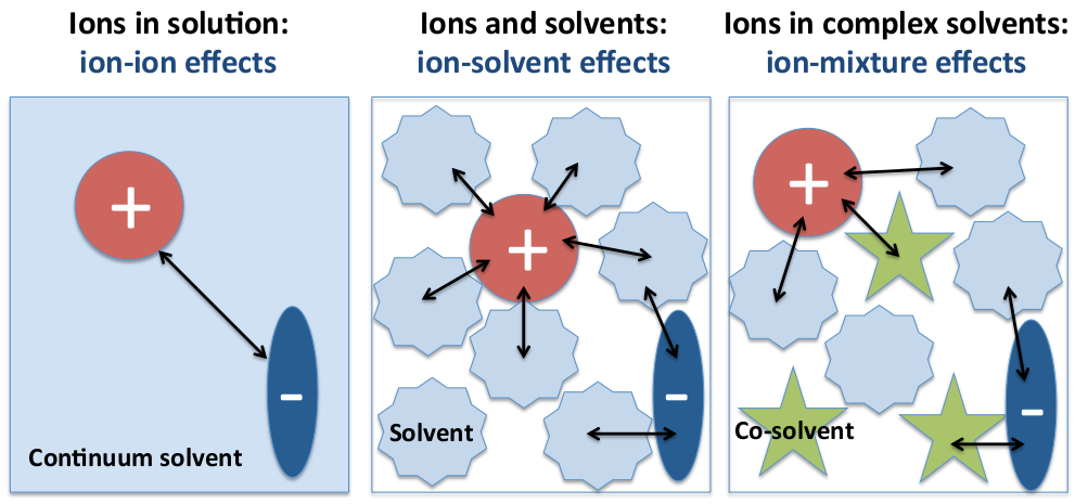
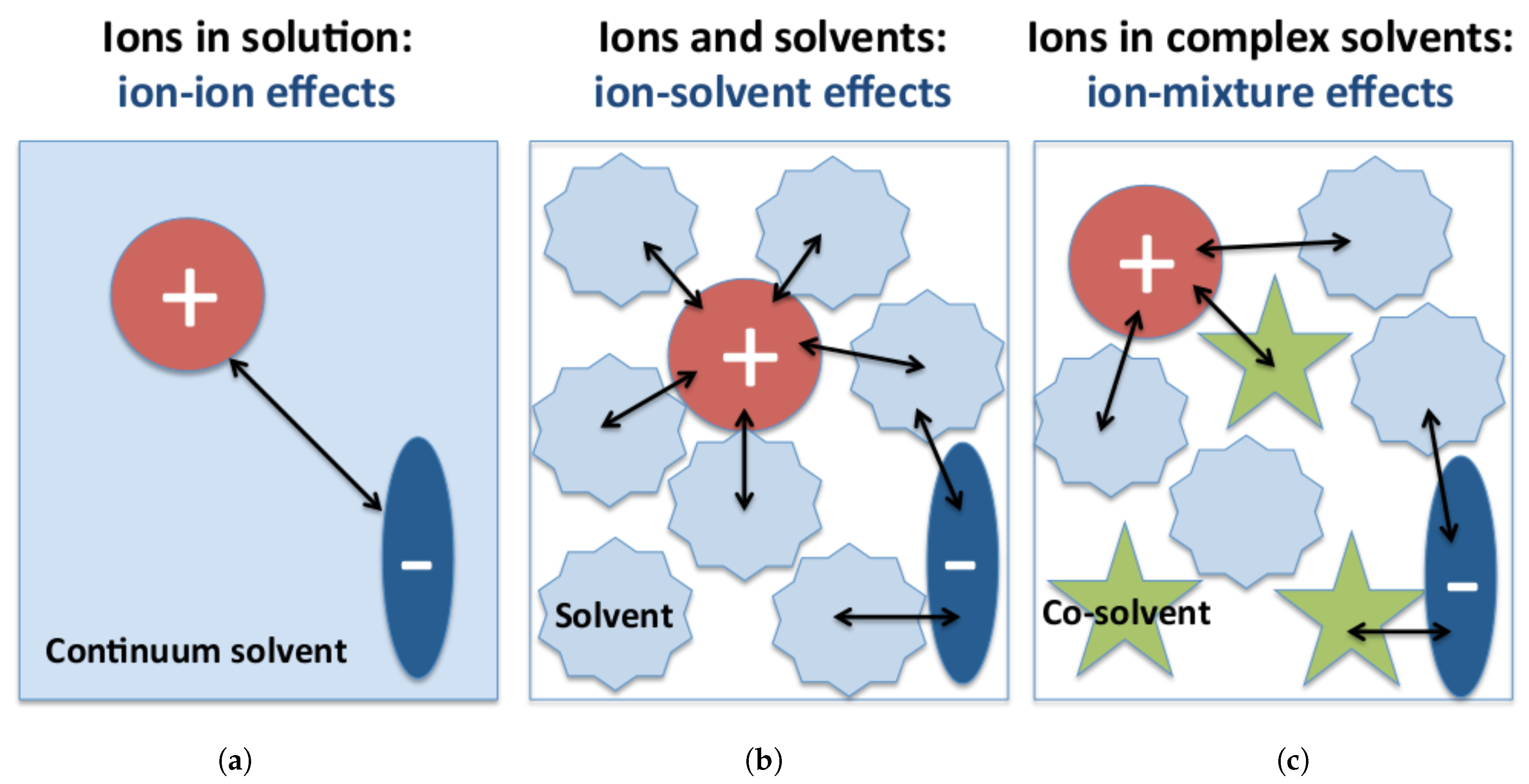
• Which factors determine ion–ion interactions, and how do the corresponding effects modify charge transport?
• Which properties of solvents are appropriate discriminators in order to distinguish between good and poor solvents, and which solvents are well-suited to increase the performance of electrochemical cells in terms of high salt solubility and beneficial charge transport behavior?
• How does the presence of co-solvents or additives affect the solvation of ions, and which conclusions can be drawn for the solubility of salts?

It has to be pointed out that most of the further important effects for electrolyte solutions, for instance chemical reactions of components at electrode interfaces, as well as the influence of strong electric fields in combination with polarization effects, are outside the scope of this review. With regard to these points, we refer the reader to further interesting and recent works besides various other studies [1,3,6,8,9,16,53,54,55,56,57,58,59].

Our article is organized as follows. With regard to Figure 1, we introduce three main sections, which focus on ion–ion interactions and the resulting consequences for charge transport, the interaction between ions and solvents, and the properties of ions in complex mixtures such as multicomponent solutions. The article starts with a basic introduction into ion correlation effects in terms of simple mean-field approaches. Hereafter, we discuss the properties of ion complex states in organic solvents and their influence on the charge transport. In Section 3, we discuss potential influences on the ion solvation behavior. In more detail, we review beneficial concepts of donor and acceptor numbers in combination with softness and hardness parameters, which provide a rational for the the occurrence of specific ion effects. The influence of co-solvents or additives on ion correlation effects is discussed in Section 4. Herein, we introduce basic concepts from KB theory in order to derive explicit expressions for the ion solubility, and the change of the chemical equilibrium between dissociated and associated ion states in presence of multicomponent solutions. At the end, we combine the concepts in order to rationalize the properties of recent electrolyte formulations, and to discuss possible routes for future research. We briefly conclude and summarize in the last section.

2. Ions in Solution: Correlation Effects and Their Influence on Charge Transport

In this section, we review basic principles regarding the properties of ions in organic solvent-based electrolyte solutions. In more detail, we discuss general concepts and highlight the crucial role of specific ion effects with regard to the underlying solvation behavior. Moreover, we introduce simple electrostatic mean-field theories and comment on their deficiencies for the description of real electrolyte solutions. At this point, we ignore the molecular details of the solvent, and thus rely on a continuum background model with a global and constant dielectric constant. The corresponding simplifications allow us to point out basic properties of ion complexes in solution. The abundant occurrence of long-range electrostatic correlation effects between the ions and the corresponding consequences for charge transport are discussed at the end of this section.

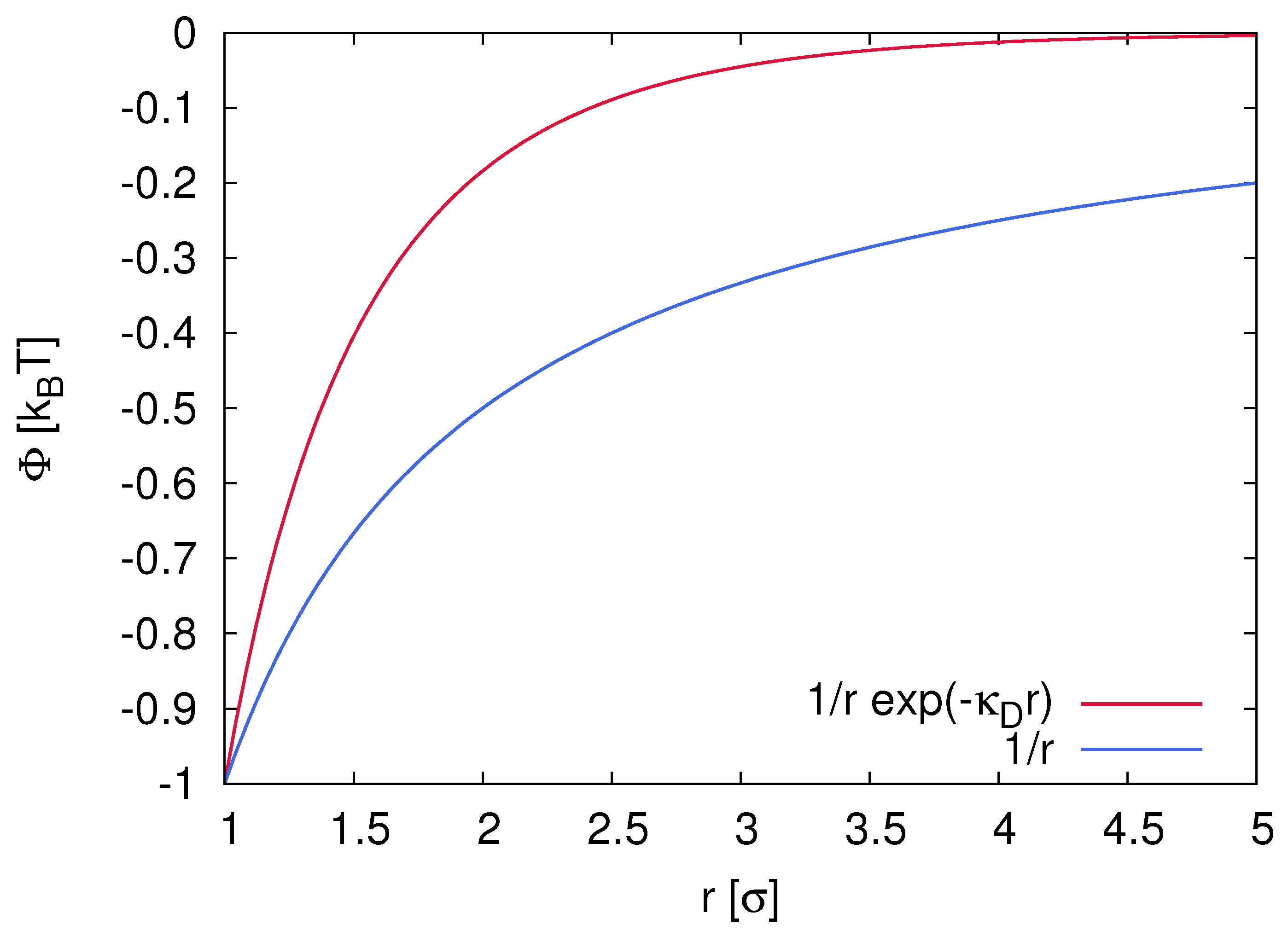
2.1. Electrostatic Interactions and Properties of Ion Complexes

The formation of ion complexes in electrolyte solutions is governed by electrostatic interactions. For two ions in a solvent with dielectric constant ${ϵ}_r$, the electrostatic Coulomb potential $\Phi \left(r\right)$ between the ions shows a decay on large length scales with [60]

$$\Phi \left(r\right)\sim 1/\left({ϵ}_{r}r\right),$$

(1)

where r denotes the distance between the ions. Note that Equation (1) is only valid for extremely dilute electrolyte solutions. At moderate and higher salt concentrations $c_s$, cations and anions mutually influence each other in terms of N-body attractive or repulsive electrostatic interactions, such that any rigorous derivation of analytical expressions without the use of reasonable approximations fails. Hence, simplifications in terms of effective field theories have to be introduced, which mostly rely on point-like ideal ions without any excluded-volume effects. Pioneering work on the properties of electrolyte solutions at finite temperature T finally brought forward the Poisson–Boltzmann (PB) theory, whose fundamental equation for ions of species j with valency $z_j$ and elementary charge e around a charged central object (main solute) can be written as [60,61,62]

$$\frac{{\partial }^2}{\partial r^2}\Phi \left(r\right)=-\sum _j\frac{z_{j}e}{{ϵ}_r{ϵ}_0}{\rho }_{j}exp\left(-\frac{z_{j}e\Phi \left(r\right)}{k_{B}T}\right)$$

(2)

with Boltzmann constant $k_B$ and vacuum permittivity ${ϵ}_0$. The density of ion species j in bulk phase at $\Phi \left(r\right)=0$ is denoted by ${\rho }_j$. It is worth noting that, even within the mean-field PB approach, analytic solutions except for simple geometries are hard to derive [60]. In contrast, for simple and dilute ions under the condition of charge neutrality $({\sum }_j{z}_j{\rho }_j=0)$, unit valency and moderate maximum electrostatic potential $\Phi \left(r_s\right)={\Phi }_s$ with ${\Phi }_s/k_{B}T\ll 1$ at the hydrodynamic boundary position $r_s$ around the main solute, Equation (2) can be linearized, which yields for the electrostatic potential around a spherical object [60]

$$\Phi \left(r\right)\sim \frac{1}{{ϵ}_{r}r}{e}^{-{\kappa }_{D}r},$$

(3)

with the Debye–Hückel length

$${\kappa }_D^{-1}=\sqrt{\frac{{ϵ}_r{ϵ}_0{k}_{B}T}{2e^2{\rho }_s}},$$

(4)

suggesting a faster decay of electrostatic interactions at finite total ion density ${\rho }_s$ when compared to single ion pairs. The corresponding decay of $\Phi \left(r\right)$ due to the presence of the surrounding ions when compared to the standard Coulomb potential for single ions (Equation (1)) is depicted in Figure 2. As can be seen, even for moderate values of the Debye–Hückel length ${\kappa }_D^{-1}=\sigma$, where $\sigma$ denotes the radius of the charged object, a significant reduction of the electrostatic potential and thus a screening effect for $r/\sigma \gg 1$ can be observed.

However, also for dilute ions in the limit of vanishing values for ${\kappa }_D$ and thus in presence of non-modified Coulomb potentials, electrostatic interactions become screened beyond a characteristic distance, which is called Bjerrum length and defined by [61]

$${\lambda }_B=\frac{e^2}{4\pi {ϵ}_0{ϵ}_r{k}_{B}T},$$

(5)

which increases with decreasing temperature and dielectric constant of the solution. In more detail, the corresponding value of the Bjerrum length denotes the distance between the ions, where electrostatic interactions are of comparable magnitude as the thermal energy $k_{B}T$. Consequently, even in the limit of vanishing salt concentrations, electrostatic interactions between the ions can be ignored for distances $r\ge {\lambda }_B$, as induced by a dielectric screening effect of the surrounding solvent molecules [63]. With regard to explicit values, water at room temperature has a value of ${\lambda }_B^{{\mathrm{H}}_2\mathrm{O}}\approx 0.7$ nm, whereas other solvents have Bjerrum lengths of ${\lambda }_B^{\mathrm{sol}}\approx 0.7·({ϵ}_r^{{\mathrm{H}}_2\mathrm{O}}/{ϵ}_r^{\mathrm{sol}})$ nm, where ${ϵ}_r^{{\mathrm{H}}_2\mathrm{O}}=78$ denotes the dielectric constant of water at room temperatures, and ${ϵ}_r^{\mathrm{sol}}$ is the corresponding value of the respective solvent. Hence, standard organic solvents in LIBs such as PC or EC with dielectric constants of ${ϵ}_r=64.92$ (PC) and ${ϵ}_r=89.78$ (EC) [1] have rather short Bjerrum lengths of ${\lambda }_B^{\mathrm{PC}}\approx 0.84$ nm and ${\lambda }_B^{\mathrm{EC}}\approx 0.61$ nm, respectively. As a simple estimate, the value of the Bjerrum length can be used to define the largest distance for electrostatically bound or correlated ions. It has to be noted that other distance criteria for ion pairs and ion complexes have also been introduced [54], but, due to reasons of simplicity, we rely on the Bjerrum length as fundamental length scale for the definition of bound ions or ion complexes without further restrictions. Previous simulation outcomes by some of us highlight the validity of this simple estimate [30,38,51,64,65,66].

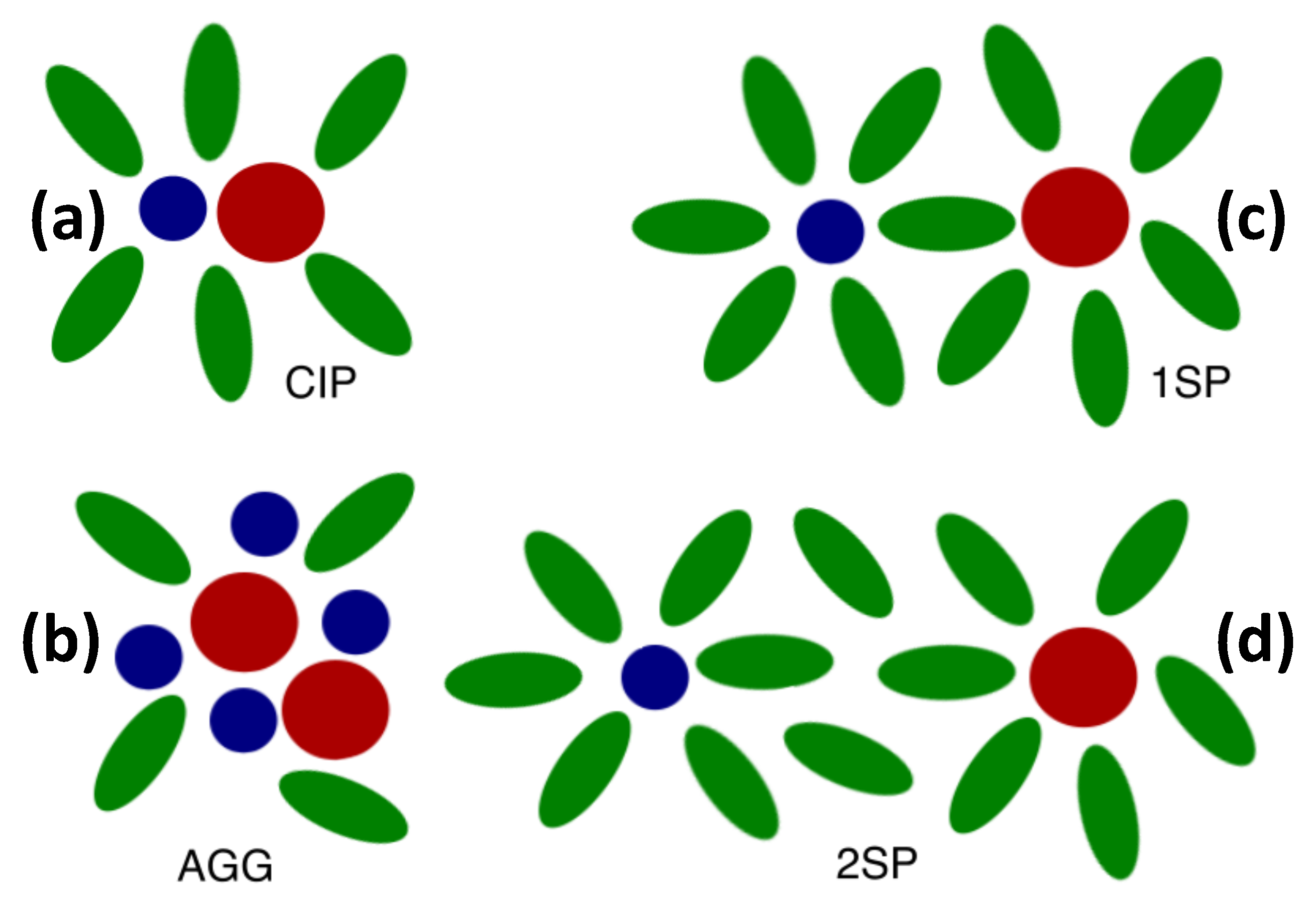
2.2. Distinct States of Ion Complexes

In contrast to simple electrostatic mean-field approaches, recent numerical and experimental findings indeed revealed the occurrence of various ion complex states. Hence, ions and solvent molecules aggregate within the Bjerrum length to ion–solvent complexes with distinct stoichiometries, as influenced by the ion species, the ion concentration, and the molecular properties of the solvent molecules [45,53,63,67,68,69,70,71,72,73,74,75,76,77,78].

In more detail, one can observe contact (CIP), solvent-shared (1SP), and solvent-separated (2SP) ion pairs in accordance with Figure 3. Despite a vast amount of current research efforts, the mechanisms underlying ion complex formation are still not fully understood [53,69,79,80,81].

In more detail, CIPs usually correspond to closest-distance contact ion pairs, whereas 1SP states include ion pairs, which are separated by one solvation shell, in contrast to 2SP states, which are separated by two or more solvation shells. Consequently, each ion in the 2SP state maintains its individual solvation shell, which is only marginally affected by the presence of the counterion. Consequently, the distance between the ions increases in the order CIP < 1SP < 2SP, which is in agreement with the reciprocal binding energies associated with the individual ion states. Despite the presence of various solvation shells [51,65], the distance between the ions in the 2SP state, as the largest complex in the aforementioned series, is always smaller than the corresponding value of ${\lambda }_B$ [70]. In terms of a moderate salt concentration of $c_s\ll 1$ mol/L, it has to be noted that most ion complexes in organic solvents are dominated by solvent-separated pairs [8,59]. The underlying reason can be attributed to the molecular details of the solvent molecules, whose coordination around the ions partly compensates the loss of electrostatic energies associated with the formation of CIP states.

At higher salt concentrations and for specific lithium salts such as lithium bis(trifluorosulfonyl)imide (LiTFSI) with bulky anions, the occurrence of ion aggregate (AGG) states in various solvents has also been observed [8,26,32,59,82]. A prominent example for AGG states are super-concentrated electrolytes or solvent-in-salt electrolyte solutions [8,26,40,59,82]. As the name “solvent-in-salt” implies, the number of solvent molecules is significantly reduced in these solutions, such that the individual solvation shells around the ions are only partially filled by solvent molecules [8,40,59]. Consequently, the number of ion complexes including CIP and AGG states increases with increasing salt concentration, although the corresponding detailed mechanisms and structures are yet under debate [82]. Over the last years, super-concentrated electrolytes for various solvents and salts [26,40,59,82] attracted enormous interest with regard to their potential use in LIBs and LMBs [8,59]. First results for acetonitrile, PC, sulfolane, and even water are promising in terms of reaching relatively high electrochemical stabilities and sufficient ionic conductivities [8,26,40,59,82].

2.3. Specific Ion Effects

For some solvents and specifically for water, differences in the complex formation tendencies for distinct ions are observed, which can be rationalized by the influence of specific ion effects [38,54,63,68,70,75,83,84,85,86]. These effects are often observed in aqueous solutions, whereas studies of specific ion effects in organic solvents are rather sparse [30,76,77,78,87]. A series of seminal studies [35,36,37] regarding the solubility of various lithium salts in acetonitrile reveals the following order, LiPF${}_6<$ LiFSI < LiTFSI $\le$ LiClO${}_4<$ LiBF${}_4\ll$ LiCF${}_3$CO${}_2$, which coincides with the observed tendency of ion complex formation.

Despite many numerical and experimental studies, a consistent theoretical framework to rationalize specific ion effects is still missing [75]. As a first empirical attempt towards this aim for aqueous electrolyte solutions, it has been proposed to distinguish ions in terms of their chaotropic and kosmotropic properties [53,54,67,68,70,73]. Hence, smaller ions such as F${}^{-}$ and Li${}^{+}$ are kosmotropes, meaning that they are water structure makers, whereas larger ions such as I${}^{-}$ and SCN${}^{-}$ are chaotropes, which emphasizes the fact that these species have to be considered as water structure breakers [53,54,63,70]. With regard to these definitions, it has to be clearly pointed out that kosmotropic and chaotropic properties are solely defined for ions in aqueous solutions, whereas the occurrence of comparable effects in aprotic solvents is currently under debate [30,76,83]. Chaotropic and kosmotropic effects on the water structure can be observed in terms of viscosity variations associated with the Jones–Dole viscosity B coefficient, as well as with regard to the dynamic behavior of water molecules in terms of dipolar relaxation times [53,63,87]. It is worth noting that recent studies on mixtures of salts with distinct properties reveal that the individual effects compensate each other [88].

As an extension of the chaotrope/kosmotrope approach, the law of matching water affinities (LMWA) was introduced by Collins [70,89], which rationalizes the experimental finding that pairs of kosmotropic or chaotropic ions reveal the highest stability. In this context, the meaning of kosmotropic and chaotropic behavior is no longer understood in terms of the impact on the water structure, rather than the degree of hydration for the corresponding ions [86]. Consequently, it is generally accepted that kosmotropes show a high degree of hydration, whereas the opposite can be assumed for chaotropic ions. The underlying empirical concept of the LMWA relies on calculated data regarding the differences of the individual ion hydration enthalpies $W_{x^{+}}$ and $W_{y^{-}}$, the so-called heats of hydration $\Delta \Delta H_{\mathrm{hyd}}=W_{x^{+}}-W_{y^{-}}$, whose difference is compared to the experimentally measurable standard heat of solution $Q_s$ of a crystalline salt with identical ions in infinite dilution. Corresponding results for distinct salts in terms of so-called volcano plots [70,83,89,90] are depicted in Figure 4A.

Hence, for $Q_s>0$, the separation of an ion pair is energetically unfavorable (endothermic reaction), whereas the ion pair easily breaks for $Q_s<0$ (exothermic reaction). With regard to the presented data, it becomes evident that ions with comparable size or influence on the water structure in terms of $\Delta \Delta H_{\mathrm{hyd}}\approx 0$ mostly reveal values of $Q_s>0$. In contrast, chaotropic and kosmotropic ions and thus ions of different size significantly differ in their individual heats of hydration according to $|\Delta \Delta H_{\mathrm{hyd}}|\gg 0$, which is most often accomplished by unstable ion pairs in terms of $Q_s<0$. Consequently, ions of comparable size show comparable degrees of hydration, so-called water affinities, such that combinations of small anions and cations or combinations of large anions and cations form the most stable ion pairs (Figure 4B [70]. For alkali halide salts, it thus can be seen that CsI with large and chaotropic ions forms the most stable ion pair. In contrast, LiI is the least stable ion pair, as it is composed of the kosmotropic lithium ion and the chaotropic iodide ion. The LMWA concept is discussed in more detail in Refs. [63,70,86,90], where it is also highlighted that electrostatic energies between the ions contribute a significant amount to the resulting values of $Q_s$. Although the presence of chaotropic properties with regard to the hydration behavior is often debated, simulation findings and experimental outcomes reveal that the complexation behavior of the ions is strongly influenced by the hydration behavior [69].

Moreover, it has to be noted that the LMWA approach reveals some similarities with the famous hard/soft acids and bases (HSAB) principle, which states that hard Lewis acids as electron acceptors prefer to coordinate with hard Lewis bases as electron donors, and soft acids prefer to coordinate with soft bases [91]. As already briefly mentioned, few studies are devoted to the occurrence of specific ion effects in non-aqueous solutions [30,38,76,77,78,83]. With regard to the corresponding results, it has been observed that the LMWA approach is also applicable for several organic solvents, such that it can be generalized to a law of matching solvent affinities [83]. Recent experimental results [78,83] thus reveal the applicability of this concept for various organic solvents such as methanol, formamide, PC, and dimethyl sulfoxide (DMSO).

In addition to the importance of these effects for lithium salts in LIBs, comparable conclusions can be drawn for sodium salts in sodium ion batteries (SIBs). In SIBs, the conducting ion is changed from Li${}^{+}$ to Na${}^{+}$, which slightly modifies the molecular interactions between the ion species, or between the ions and the solvent molecules. In fact, the differences in the solvation behavior between Li${}^{+}$ and Na${}^{+}$ in most organic solvents are rather marginal, which can be rationalized by the low charge of both ions. Hence, it has been discussed that identical solvents or anions such as in LIBs can be used in SIBs [10]. Despite recent successful efforts with regard to new materials, it has to be mentioned that SIBs provide lower energy densities when compared to LIBs due to a higher standard electrode potential of Na${}^{+}$ in contrast to Li${}^{+}$ besides other drawbacks [92]. In contrast, the properties of salts with divalent or trivalent ions change significantly when compared to lithium or sodium salts. It has been reported that the transfer of multivalent ions from water to organic solvents is highly unfavorable, as evidenced by positive transfer free energies [93]. Furthermore, multivalent ions show a high preference being in contact with water molecules, which hinders systematic studies on ion pairing and ion association in hygroscopic organic solvents. In contrast to monovalent ions, the association tendency of multivalent ions is also significantly increased, which can be rationalized by stronger electrostatic interactions between the ion species. As a specific example, it has been shown that large objects reveal a charge reversal behavior in presence of multivalent ions, which means that more ions are bound than needed for charge compensation [94,95].

2.4. Ion Correlation Effects and Transport Behavior

With regard to the previous discussion in Section 2.2, we now demonstrate why the occurrence of ion complexes is of fundamental importance for electrolyte research. As prime example, the formation of ion complexes heavily affects the ionic conductivity due to omnipresent correlations between the ions. Strictly speaking, ions which form net neutral complexes, as mentioned before, do not contribute to the ionic conductivity, which negatively affects the power density of electrochemical cells. It is thus beneficial to achieve high values of ion dissociation, which is usually supported by using high dielectric constant solvents [1].

With regard to the influence of ion correlations on charge transport, the ideal ionic conductivity for non-interacting, i.e., ideal, ions is given by the Nernst–Einstein equation, which for a 1:1 salt in the limit of long times reads [96,97]

$${\sigma }^{\mathrm{id}}=\frac{e^2{\rho }_s}{k_{B}T}(D_{++}^s+D_{--}^s)$$

(6)

where $D_{++}^s$ and $D_{--}^s$ denote the individual self-diffusion coefficients for cations and anions. With regard to the presence of ion complexes, it becomes obvious that Equation (6) is only valid in the limit of low salt concentrations due to negligible ion correlation effects. Hence, for higher salt concentrations, the effective, or experimentally observed, ionic conductivity in terms of the Einstein–Helfand equation [51,65,66,96,98] reads

$${\sigma }^{\mathrm{eff}}=\frac{e^2{\rho }_s}{k_{B}T}(D_{+}+D_{-}).$$

(7)

with

$$D_{+}\equiv D_{++}^s+D_{++}^{\prime }-D_{\pm }$$

(8)

and

$$D_{-}\equiv D_{--}^s+D_{--}^{\prime }-D_{\pm }$$

(9)

where $D_{--}^{\prime }$ and $D_{++}^{\prime }$ denote the cross-correlated diffusion coefficients between cations or anions, respectively, and $D_{\pm }$ the corresponding symmetric diffusion coefficients including correlation effects between anions and cations. As can be seen, the contributions of $D_{\pm }$ diminish the effective ionic conductivity considerably when compared to the ideal ionic conductivity. Consequently, the ideal Nernst–Einstein ionic conductivity suffers from a neglect of ionic correlations, such that Equation (6) provides the maximum possible ionic conductivity in accordance with ${\sigma }^{\mathrm{id}}>{\sigma }^{\mathrm{eff}}$.

In addition, the calculation of ideal and effective ionic conductivities allows us to estimate the amount of correlated ion motion. As a specific expression for the dynamic correlation factor, the ratio of both ionic conductivities reads [96,98]

$${\Delta }_{\mathrm{IC}}=1-\frac{{\sigma }^{\mathrm{eff}}}{{\sigma }^{\mathrm{id}}}$$

(10)

with ${\Delta }_{\mathrm{IC}}\in [0,1]$, where a value of ${\Delta }_{\mathrm{IC}}=1$ reveals full ion correlation, and vice versa ${\Delta }_{\mathrm{IC}}=0$ the absence of any correlation effects. It has to be pointed out that the value of ${\Delta }_{\mathrm{IC}}$ represents the fraction of correlated ion motion, which does not necessarily coincide with the fraction of ion complexes. As discussed in Section 2.2, all CIP, AGG, 1SP and 2SP states are examples of ion complexes and thus contribute to the actual value of the dynamic correlation factor. A further distinction between the individual contributions regarding the value of ${\Delta }_{\mathrm{IC}}$ is hence not obvious without any detailed analysis of the structural arrangement.

In addition to the ionic conductivity, the cation transference number as a further descriptor of charge transport [9]

$$t^{+}=\frac{{\sigma }_{+}^{\mathrm{eff}}}{{\sigma }^{\mathrm{eff}}}$$

(11)

with

$${\sigma }_{+}^{\mathrm{eff}}=\frac{e^2{\rho }_s}{k_{B}T}{D}_{+}$$

(12)

is also of fundamental importance for LIBs or LMBs, as it mainly determines the charging and discharging rates. For highly effective electrolyte solutions or single ion conductors, one can observe values of $t^{+}>0.5$ [9,97], whereas most values in organic liquid electrolyte solutions are $t^{+}<0.5$ [6,9]. The corresponding value reveals that anions instead of cations mostly contribute to the ionic conductivity as an unwanted side effect in organic solvent-based LIBs. In the limit of negligible ion correlations or low salt concentrations, the cation transference number coincides with the cation transport number ${lim}_{{\Delta }_{\mathrm{IC}}\to 0}{t}^{+}=t_{\mathrm{app}}^{+}$, which is defined by [96,99]

$$t_{\mathrm{app}}^{+}=\frac{D_{++}^s}{D_{++}^s+D_{--}^s}$$

(13)

and hence ignores any correlation effects. Experimental results reveal significant deviations between transference and transport numbers, which highlights the influence of correlation effects for charge transport mechanisms in external electric fields [99,100,101]. Consequently, the formation of ion complexes at high and moderate salt concentrations imposes a significant limitation on ionic conductivities and on transference numbers. As these values are of fundamental importance for the electrochemical performance of LIBs, it is thus desirable to minimize these effects considerably [9].

As an example for charge transport in adiponitrile, the values of ideal and effective ionic conductivities at 300 K by means of atomistic molecular dynamics (MD) simulations in comparison to experimental values for different concentrations of LiBF${}_4$ and LiTFSI are shown in Figure 5 [30].

In agreement with the Walden relation [63], which reads ${\sigma }^{\mathrm{id}}\sim c_s/\eta$, where $\eta$ is the shear viscosity of the solution following from insertion of the Stokes–Einstein equation with $D^s\sim 1/\eta$, one observes a linear increase of the ionic conductivity at low salt concentrations due to ${\Delta }_{\mathrm{IC}}\approx 0$. At moderate concentrations, a maximum value of the ionic conductivity can be observed in terms of a balance between ion correlation effects and a high amount of charge carriers. In agreement with the limiting law for the ionic conductivity at very high salt concentrations [102,103] with $\sigma ={\sigma }_0-\xi c_s^{3/2}$, the values for the ionic conductivity reveal a nonlinear decay due to a positive Onsager prefactor $\xi$. With regard to the values for the effective Einstein–Helfand ionic conductivity, as shown in Figure 5, it can be concluded that the smaller BF${}_4^{-}$ anion induces a higher tendency of ion complex formation when compared to the TFSI${}^{-}$ anion, which is in agreement with the LMWA and HSAB concept. Further analysis reveals that both anions have comparable values for self-diffusion constants, and thus comparable ideal Nernst–Einstein ionic conductivities, which highlights the fact that the differences in the ionic conductivity can be solely attributed to ion correlation effects [30].

A simple and fast computation of ionic conductivities is provided by the advanced electrolyte model [104]. The corresponding approach strongly relies on the influence of different ion motion contributions, and also considers the complexation behavior of the ions. The validity of the model has recently been demonstrated for a series of ion and solvent combinations [105]. Ion correlation effects are also observed in polymer electrolytes, which are often considered as potential components of solid state batteries. In Reference [106], it is observed that, in mixtures of poly(ethylene oxide) (PEO) and LiI salts, correlated motion between the ions occurs, which differs significantly from previous findings for organic solvents. As the lithium ions are strongly coordinated by the oxygen atoms of the PEO chain, distinct spatiotemporal correlations dominate, which can be separated into several contributions in terms of the total dynamic behavior. However, the correlation between lithium and iodide ions contributes most significantly to the dynamics, which can be brought into agreement with simple analytic models by the introduction of phenomenological parameters.

All findings reveal that ion correlation effects are omnipresent, and dominate the dynamics of distinct systems at high salt concentrations. A deeper understanding of ion complex formation principles is thus of fundamental importance in order to develop improved electrolyte solutions.

3. Solvent–Ion Interactions at the Molecular Scale

In this section, we discuss the properties of solvents and their influence on the formation of ion complexes in more detail. Ion–solvent interactions are dominated by several factors, which are reviewed in the following subsections in terms of several examples.

3.1. Dielectric Decrement Effects

As discussed in Section 2.2 and Section 2.4, electrostatic attraction drives the formation of ion complexes, whose occurrence reduces the ionic conductivity due to correlation effects. In terms of a simple solution to this problem, the Bjerrum length for the respective solvents should have low values as achieved by high values for the dielectric constant ${ϵ}_r$. The question arises: Which molecular factors affect the dielectric constant of a solvent? Besides more sophisticated Green–Kubo relations [51,65,98], a simple relation for the dielectric constant reads [107,108,109]

$${ϵ}_r=1+4\pi \frac{\langle M_{\mathrm{trans}}^2\rangle }{3V{k}_{B}T}$$

(14)

which is readily applicable for one-component mixtures by the evaluation of the time-averaged squared net total translational dipole moment $\langle M_{\mathrm{trans}}^2\rangle$ of the molecules in the respective volume V. Consequently, well-arranged polar solvents with pronounced molecular dipole moments show a high value of the dielectric constant, and are thus beneficial media to reduce ion correlation effects.

Despite this simple view, it has to be mentioned that the value of the dielectric constant also depends on the chosen position, as it can locally change in close vicinity to ions, uncharged solutes, interfaces, and due to inhomogeneities in the solution [64,110,111,112,113]. Moreover, it is also affected by solvent–solvent, solvent–ion, and ion–ion interactions, which contribute significantly to the net value of the dielectric constant. However, for dilute salt conditions, a recent publication reports that the dielectric constant is mostly affected by solvent–solvent instead of ion–solvent or ion–ion contributions [51]. Although the corresponding findings significantly change at molar salt concentrations [64,66,81], the use of high dielectric constant solvents still remains beneficial.

To rationalize the change of the dielectric constant around charged objects such as ions, one has to remember that the electrostatic field of the ions perturbs the relaxation of the surrounding solvent molecules in terms of multipole interactions in accordance with [63]

$${ϵ}_r\left(E_{\varphi }\right)={ϵ}_r+\beta E_{\varphi }^2,$$

(15)

where ${ϵ}_r\left(E_{\varphi }\right)$ denotes the modified dielectric constant of the solvent due to a solvent- and concentration-specific coupling constant $\beta <0$ in combination with the electrostatic field $E_{\varphi }$. It is worth noting that the corresponding variation of ${ϵ}_r\left(E_{\varphi }\right)$, which is called dielectric decrement effect, thus affects the Coulomb energy between ions, and hence promotes the formation of ion complexes due to larger values of the Bjerrum length. Consequently, the Bjerrum length for polar solvents often increases in presence of higher salt concentrations. Furthermore, polar solvent molecules are strongly bound to the ion, which results in compression effects in terms of electrostriction mechanisms [63], which also diminish the mobility of the ions.

Consequently, the dielectric decrement effect can be considered as an important example for crucial solvent–ion interactions at local scales. Whereas these findings are of minor importance for low salt concentrations, their importance increases drastically at higher concentrations, as most solvent molecules are now part of the first or second solvation shell around the ions [64,66,114]. Thus, strongly bound solvent molecules govern the global properties of the solution, and thus also decrease the overall ionic conductivity in combination with stronger electrostatic correlation effects.

3.2. Molecular Properties of the Solvent: Donor/Acceptor Numbers and Chemical Hardnesses

The results of mean-field theories with a dielectric continuum solvent approach imply that solvents with low Bjerrum lengths induce a lower tendency of ion complex formation. In contrast, recent experimental and atomistic molecular dynamics (MD) simulation results highlighted a more complex behavior [38,87]. As an illustrative example [87], the counterion condensation behavior for sodium ions around highly charged sulfonated oligosulfonic acids in different solvents water, dimethyl sulfoxide (DMSO) and chloroform is shown in Figure 6. With regard to electrostatic mean-field counterion condensation theories [115,116,117], one would expect that the number of bound counterions increases with the order water < DMSO < chloroform in accordance with decreasing Bjerrum lengths [87].

Despite this reasonable assumption, it can indeed be seen in Figure 6 that more sodium ions are bound to the polyelectrolyte in water when compared to DMSO, which implies the following order for the fraction of bound counterions, DMSO < water < chloroform, such that water and DMSO change their positions. Hence, the corresponding results reveal that some solvents induce a strong counterion condensation behavior, which does not agree with the corresponding value of the dielectric constant nor Bjerrum length.

Hence, it is concluded that the amount and the interaction energy of coordinating solvent molecules in the first solvent shell around the ions reveal a massive influence on the solubility of the ions, and thus also on the formation tendency of ion complexes and the underlying free solvation energy [87]. In contrast to these enthalpic interactions, entropic contributions in terms of solvent conformations only account for around 10–20% [38] of the ion free solvation energy, and are thus of minor importance for most solvent–ion interactions [63]. The overwhelming remainder of the aforementioned enthalpic contributions can be assigned to ion–dipole interactions in presence of polar solvent molecules. Comparable findings were reported for adiponitrile [30]; for the different solvents water, N,N-dimethylacetamide, methanol, PC and EC [30,118]; and for lithium salts in presence of urea [119].

To discuss the results of Figure 6 in more detail, it is well-known that DMSO has two lone pair electrons, which imply a high nucleophilicity of the molecule, and thus very likely interact with positively charged groups or cations. The nucleophilic behavior of DMSO is even more pronounced when compared to water, which is a more favorable anion solvent due to its protic properties. Thus, in addition to the value of the dielectric constant, distinct polar solvent molecules have nucleophilic or electrophilic properties, which significantly influence the solvation behavior of anions and cations.

To categorize solvents with regard to their cation solvation properties, Gutmann et al. introduced the so-called empirical donor number (DN) [63,120,121], which accounts for the electron donating properties (donicity) of a solvent molecule. The value of the donor number DN is defined as the negative reaction enthalpy in units of kcal/mol for antimony pentachloride with the respective solvent in a 1:1 ratio in inert solvent 1,2-dichloroethane. It has to be noted that sometimes a donor number is also assigned to ion species, but, to keep the discussion simple, we merely focus on DN values for solvents [122].

As few examples, the values of donor numbers for common solvents are shown in

Table 1. Donor numbers (DN), acceptor numbers (AN), and values for the softness parameter ($S_{\exp }$) for common solvents according to Refs. [63,123,124,125,126,127]. Unknown values are denoted by $n.a.$

Solvent	DN	AN	${\mathit{S}}_{\mathbf{exp}}$
Water	18.0	54.8	0.0
Propylene carbonate	15.1	18.3	−0.09
Ethylene carbonate	16.4	$n.a.$	$n.a.$
Dimethyl carbonate	17.2	$n.a.$	$n.a.$
Diethyl carbonate	16.0	$n.a.$	$n.a.$
1,2–dimethoxyethane	20.0	$10.2$	$n.a.$
1,3–dioxolane	21.3	$n.a.$	$n.a.$
Tetraethylene glycol dimethyl ether	16.6	$10.5$	$n.a.$
N,N–Dimethylformamide	26.6	16.0	0.11
N,N–Dimethylacetamide	27.8	13.6	0.17
Dimethyl sulfoxide	29.8	19.3	0.22
Chloroform	4.0	23.1	$n.a.$
Tetramethylene sulfone	14.8	19.2	0.00
Methanol	30.0	41.5	0.02
Ethylene glycol	20.0	43.4	−0.03
Acetonitrile	32.0	18.9	0.34
N–Propanol	30.0	33.7	0.16
1,4–Dioxane	14.8	10.8	0.07
$\gamma$–Butyrolactone	18.0	17.3	0.02
N–Methylformamide	27.0	32.1	0.17
N,N–Dimethylformamide	26.6	16.0	0.11
N,N–Dimethylacetamide	27.8	13.6	0.17
Pyridine	33.1	14.2	0.64
Benzonitrile	11.9	15.5	0.34

. The highest values of DNs can be observed for pyridine and acetonitrile, which are thus beneficial solvents in order to solvate cations. In contrast, chloroform has to be considered as a poor solvent in this regard. In fact, the DN values for DMSO, water, methanol, chloroform, and N,N-dimethylacetamide also exactly follow the order observed for the ion binding behavior around polyelectrolytes, as discussed above and in Refs. [51,87]. Finally, all standard carbonate-based solvents and co-solvents of LIBs reveal sufficient DN values around 15–20 (Table 1).

Moreover, Table 1 also shows the values for the Gutmann–Mayer acceptor number (AN). The acceptor number accounts for the electron accepting properties (electrophilicity) of the solvent molecules. This property is closely related to the protic properties of a solvent, i.e., its tendency to donate protons in order to form hydrogen bonds or salt bridges with the anions, which rationalizes the high values for water (AN = $54.8$). The corresponding AN values are obtained by using NMR chemical shift values of $\delta$ for the ${}^{31}$P atom of triethylphosphine oxide in the respective solvent relative to the shift in N–hexane [63]. All AN values are commonly normalized to assess AN = 2.348 ($\delta$/ppm), meaning that the $\delta$-values are corrected for the diamagnetic susceptibility ${\chi }_s$ of the solvent. Consequently, a suitable solvent to reduce the formation of ion complexes between cations and anions should have high values of AN and DN, in combination with a low viscosity and a high dielectric constant. Although exact predictions within the donor and acceptor number concept are hard to derive, the DN and AN values provide a reasonable framework to identify suitable solvents for specific salts.

Closely related with the donor number is the Kamlet–Taft (KT) ${\beta }_{\mathrm{KT}}$ scale [63], which relies on mean values obtained from protic solvatochromic probes in comparison to structurally similar aprotic probes. The corresponding values ${\beta }_{\mathrm{KT}}$ are normalized to the interval defined by 0 (cyclohexane) and 1 (hexamethylphosphoric triamide). Values from KT and DN scales can be transformed via the relation

$$\mathrm{DN}=38.2{\beta }_{\mathrm{KT}}+0.5$$

(16)

as outlined in detail in Ref. [63]. However, it has to be noted that DN, AN, and ${\beta }_{\mathrm{KT}}$ values usually fail in terms of the solvation behavior of ions in multicomponent solutions [51,65]. Consequently, AN and DN values provide a reasonable starting point to estimate the quality of ion solvation in the respective single solvents at low salt concentration.

Furthermore, the interaction strength between the ions and the solvent is intimately linked to the corresponding polarizabilities of the components. With regard to this remark, specifically the chemical hardness/softness of the solvent and the ions are discussed as a potential discriminator for beneficial ion–solvent and ion–ion combinations [63]. Herewith, a connection to the HSAB principle [91] and the closely related LMWA approach [70,89] can be drawn straightforwardly. Strict definition of chemical hardness or softness are provided in the context of conceptual density functional theory (DFT) [128,129,130,131]. As a prerequisite, it can be rigorously shown that the electronegativity of a molecule or ion can be defined as [128]

$$\chi =-{\left(\frac{\partial E}{\partial n}\right)}_{\mathcal{V}}$$

(17)

as the derivative of the total electronic energy functional E with the number of electrons n under the constraint of a constant external or nuclear potential $\mathcal{V}$. Hence, the hardness of a species, whose value can be interpreted as resistance against electronic changes, follows from [128,131]

$${\eta }_H={\left(\frac{{\partial }^{2}E}{\partial n^2}\right)}_{\mathcal{V}}=-{\left(\frac{\partial \chi }{\partial n}\right)}_{\mathcal{V}},$$

(18)

which is the inverse of the softness [131]

$$S=\frac{1}{{\eta }_H}$$

(19)

in order to discriminate between polarizable and unpolarizable molecules [128]. As a simple estimate, the hardness and thus also the softness of a species can be estimated by the relation [129,131]

$${\eta }_H\simeq E_{\mathrm{LUMO}}-E_{\mathrm{HOMO}}$$

(20)

in terms of highest occupied and lowest unoccupied orbital energies $E_{\mathrm{HOMO}}$ and $E_{\mathrm{LUMO}}$, respectively. Consequently, species with small energy gaps between $E_{\mathrm{HOMO}}$ and $E_{\mathrm{LUMO}}$ are soft and thus easily polarizable, whereas the presence of large energy gaps is a property of hard species. Moreover, pronounced values of $|E_{\mathrm{HOMO}}|\gg 0$ coincide with a high oxidative stability in accordance with the Koopmans theorem [132,133], which implies that hard solvents such as adiponitrile can be used in high voltage LIBs without significant degradation effects [30].

In addition to computational studies and with regard to experimental measurements, the softness of ions can also be estimated by the difference of the formation energies in the gas phase (loss or gain of electrons), and the transfer energy of the respective ions from gas phase to aqueous solution [63]. Consequently, the closely related softness parameter $S_{\exp }$ for solvents relies on the evaluation of the transfer free energy $\Delta G_{\mathrm{tr}}^0=\Delta G_{\mathrm{solv}}^0-\Delta G_{\mathrm{aq}}^0$ for standardized ions from water as the source solvent (aq) to the solvent of interest (solv). In terms of standard ions from a well-defined experimental reference system, one usually relies on soft silver ions, on the one hand, and averaged values for hard sodium and potassium ions, on the other hand. Consequently, the empirical softness parameter for solvents can be calculated by [63]

$$S_{\exp }=\left[\Delta G_{\mathrm{tr}}^0\left({\mathrm{Ag}}^{+}\right)-1/2\left(\Delta G_{\mathrm{tr}}^0\left({\mathrm{Na}}^{+}\right)+\Delta G_{\mathrm{tr}}^0\left({\mathrm{K}}^{+}\right)\right)\right]/\left(100\mathrm{kJ}/\mathrm{mol}\right)$$

(21)

whereas other definitions and reference ions are also used [63]. In terms of Equation (21), solvents with $S_{\exp }\ge 0.25$ are considered as soft solvents, and thus preferably solvate soft ions, whereas solvents with $S_{\exp }\le 0$ are regarded as hard solvents, and thus preferably solvate hard ions. As shown by the values in Table 1 and in agreement with Equation (21), pyridine is a soft solvent, whereas PC and ethylene glycol are hard solvents. Furthermore, and despite the high DN value, pyridine is a rather poor solvent for lithium ions as one of the hardest ion species. Moreover, the roughly similar DN and AN values in combination with its pronounced chemical hardness rationalize the abundant use of PC as common component in LIB electrolyte solutions.

3.3. Solvation of Ions: Benefits of Computational Approaches

In combination with experimental studies, computational approaches are powerful tools which provide detailed insight into molecular interactions as well as electrochemical stabilities [17,55,56,82,132,133]. Closely connected with the conceptual DFT approach, numerical studies on the solvation behavior of lithium salts in organic solvents mostly rely on quantum chemical calculations in terms of DFT computations [55,56,57]. Here, we briefly discuss some standard protocols for reasons of completeness.

As a common approach to study the strength of ion–solvent interactions, the ions are surrounded by a local solvent cluster in accordance with the assumed first solvent shell coordination number [55]. Most often, the ion–solvent cluster is also embedded into a local continuum background with global dielectric constant to increase the accuracy of the calculations. With regard to this attempt, the lithium ion solvation energy can be computed by [56,134]

$$\Delta E_{\mathrm{solv}}=E_{\mathrm{tot}}({\mathrm{Li}}^{+}·S_x)-E_{\mathrm{tot}}\left({\mathrm{Li}}^{+}\right)-x·E_{\mathrm{tot}}\left(S_x\right),$$

(22)

with $E_{\mathrm{tot}}({\mathrm{Li}}^{+}·S_x)$ as total potential energy between the lithium ion and x solvent molecules ($S_x$), the total lithium ion energy $E_{\mathrm{tot}}\left({\mathrm{Li}}^{+}\right)$, and the total energy of $x=1,\dots ,N_s$ solvent molecules without ions $E_{\mathrm{tot}}\left(S_x\right)$. The number x of coordinating solvent molecules around the lithium ions can be estimated from Raman spectroscopy measurements, or from previous atomistic molecular dynamics (MD) simulations.

In addition to the solvation energy, the total desolvation energy, meaning the energy that is needed to remove the solvent shell from the lithium ions reads [56,134]

$$\Delta E_{\mathrm{desolv}}=E_{\mathrm{tot}}({\mathrm{Li}}^{+}·S_x)+E_{\mathrm{tot}}\left(S_x\right)-E_{\mathrm{tot}}\left([{\mathrm{Li}}^{+}·S_{x-1}]\right)$$

(23)

which can be computed for an arbitrary value of x solvent molecules. A corresponding example is shown in Figure 7, where different clusters of lithium ion–EC complexes (${[\mathrm{Li}·S_{x=1-4}]}^{+}$) are depicted. After geometry-optimization, the corresponding values for the total energy can be calculated with regard to adequate DFT functionals and basis sets. In terms of computational efficiency, B3LYP and PBE functionals often provide reasonable values [135], whereas more sophisticated Gaussian correlated G4MP2 approaches are nowadays also often in use [55,82]. However, it has to be noted that dispersion interactions are ignored in simple DFT calculations [136], and have to be taken additionally into consideration, specifically with regard to large solvent–ion clusters [136,137,138].

In addition to potential energies (enthalpies), the corresponding free energies for the ion–solvent clusters can also be evaluated via the relation [135]

$$G=E+\mathrm{ZPE}+pV-RTln\tilde{\Sigma }$$

(24)

where ZPE denotes the zero point energy, R denotes the universal gas constant, $pV$ denotes the pressure–volume relation, and $\tilde{\Sigma }$ denotes the molecular partition function with zero ground state energy. The corresponding values can be obtained from an a posteriori vibrational frequency analysis [139]. Additional evaluation of electrochemical stabilities in terms of redox potentials by the use of the Nernst equation highlight the applicability of the approach for distinct solvents in good agreement with experimental results [55,132,133].

Although quantum chemical approaches at different levels of theory are useful to estimate the binding energies and the corresponding oxidation and reduction potentials to a sufficient extent, limited information on the dynamic behavior of the complexes is available with regard to such static approaches. Moreover, and due to large computational costs, only the first or second coordination shells around the ions are taken into consideration. However, from our previous discussion in Section 2.2, it can be concluded that the associated length scales are often too short to properly reflect long-range electrostatic interactions. Thus, although aiming to provide a high degree of accuracy, quantum chemical calculations often suffer from finite volume effects or slight numerical variations due to the use of inappropriate functionals. The results of these calculations are rough estimates, which have to be underpinned and verified by experimental measurements or sophisticated MD techniques.

4. Ions in Multicomponent Solutions: Influence of Co-Solvent and Additive Molecules on the Properties of Ion Complexes

In Section 3, we discuss the properties of ions in single solvents. As shown, the molecular details of the solvent molecules and further specific properties such as the chemical hardness and the DN/AN values are of fundamental importance. However, the underlying considered binary solution, as composed by the dissolved salt and the solvent, reveals a rather low level of complexity. In this section, we focus on the influence of additional components in terms of co-solvents or additive molecules. Useful theoretical approaches to unravel these complex properties are molecular theories of solutions such as the Kirkwood–Buff (KB) theory or inhomogeneous fluctuation theory [34,41,42,45,51,140], which provide a straightforward definition of basic thermodynamic concepts in regards of molecular distribution functions. This section aims to introduce the basic framework and to highlight the benefits of the considered approaches for the study of multicomponent solutions.

It is worth noting that standard electrolyte formulations in LIBs are indeed often composed of distinct lithium salts, solvents, co-solvents, and several additive components. Besides further tasks, these additional compounds are often introduced to increase the solubility of the lithium ion conducting salt, and to decrease the viscosity of the solution [1,3,4,141]. With regard to both aims, often a high dielectric constant solvent such as EC or PC, which usually suffers from a high viscosity [6], is combined with co-solvent or additive components to decrease the viscosity of the solution, and thus enhance charge transport. Unfortunately, typical co-solvents such as EMC or DMC reveal low dielectric constants, which crucially supports the occurrence of ion correlation effects at higher co-solvent concentrations. In more detail, for low co-solvent concentrations, one usually observes a significant increase of the ionic conductivity due to decreasing viscosities in regards of ${\sigma }^{\mathrm{eff}}\sim 1/\eta$ until a maximum value is reached. For higher co-solvent concentrations, the influence of the main high dielectric constant solvent on the solubility of the salt decreases, such that the higher amount of co-solvent molecules induces an increase of ion correlation effects, which negatively affects the ionic conductivity in terms of the dynamic correlation factor (Equation (10)). The question arises: How can the presence of co-solvent molecules induce a change of ion correlation effects? With regard to our previous discussion in Section 3, it can be assumed that local interactions between the co-solvent molecules and the ions are mainly responsible for the observed variations.

4.1. Molecular Theories of Solution: Co-Solvent–Ion Interactions

To clarify this question in more detail, one has to study the composition of the solvent shells around the ions as well as the general distribution of species in the solution. Beneficial approaches in this context are molecular theories of solution, and specifically the Kirkwood–Buff (KB) theory [34,41,42,45,52]. As one would assume, a good solubility of ions in mixtures can be achieved by a preferential coordination of highly polar molecules around the ions, whereas the more apolar species should remain in bulk solution [1,3]. This simple view can be associated with a preferential solvation behavior, which can be studied straightforwardly by means of KB theory. Hence, if both ion species are preferably solvated by either solvent or co-solvent molecules, meaning that only one species forms the vast majority of the first solvation shell around both ions, the corresponding behavior is called homoselective solvation. In contrast, if both ion species are solvated by distinct components, which means that the first solvation shells around the ions differ significantly, a heteroselective solvation behavior can be observed. Furthermore, if the minor component of the solution, meaning the co-solvent or additive molecules, is excluded from the first ion solvation shell, one usually describes this observation as a preferential exclusion behavior, whereas a significant accumulation in close vicinity around the ions is called preferential binding [45,52]. After having defined basic principles of ion solvation in multicomponent solution, we now outline some fundamental concepts of KB theory in order to discuss the influence of co-solvent molecules on the ion dissociation behavior in more detail.

4.2. Ion Complexes in Presence of Co-Solvent Molecules: Influence on the Ion Dissociation Equilibrium

To study the influence of co-solvent molecules on the ion dissociation–association chemical equilibrium or the closely related salt solubility, we start this section with a simple ion dissociation–association reaction in terms of

$$\left({\mathrm{X}}^{+}{\mathrm{Y}}^{-}\right){}_{\mathrm{sol}}\rightleftharpoons {\mathrm{X}}_{\mathrm{sol}}^{+}+{\mathrm{Y}}_{\mathrm{sol}}^{-}$$

where the ion complex, either CIP, 1SP, 2SP or AGG, as defined in Section 2.2, is denoted by (X${}^{+}$Y${}^{-}$)${}_{\mathrm{sol}}$, and the fully dissociated ions by X${}_{\mathrm{sol}}^{+}$ and Y${}_{\mathrm{sol}}^{-}$. In principle, a lower amount of ion complexes can be achieved if the chemical equilibrium is significantly shifted to the right side, such that the solvation of the individual ion species is enhanced. For a theoretical description of this effect, we assume the presence of an infinitesimally small ion concentration, and we do not distinguish between CIP, 1SP, 2SP and AGG states. Thus, all ions within the Bjerrum length are considered as associated ion complexes, whereas all other ions are considered as dissociated ions [51]. In addition, the chemical equilibrium constant K is defined by the relations [142] $\Delta \mu ={\sum }_j{\omega }_j{\mu }_j=0$ and

$$\Delta {\mu }^0=\sum _j{\omega }_j{\mu }_j^0=-RTlnK,$$

(25)

with the chemical potentials ${\mu }_j$, the standard chemical potentials ${\mu }_j^0$, and the stoichiometric coefficients ${\omega }_j$ [142]. With regard to Equation (25), the chemical equilibrium constant can also be written as [142]

$$K=\prod _j{a}_j^{{\omega }_j}$$

(26)

with the chemical activity $a_j={\gamma }_j{x}_j$, where ${\gamma }_j$ denotes the chemical activity coefficient in combination with the mole fraction $x_j$. In terms of nomenclature, the salt ions have index “2”, whereas the solvent and co-solvent molecules have indices “1” and “3”, respectively. Within standard KB theory, it has to be noted that cations and anions have to be considered as indistinguishable [45,46,143].

If a linear influence of co-solvent molecules on the chemical equilibrium and on the chemical potential of the ions is assumed, it follows [42,45,51,144]

$$\Delta {\mu }_{\mathrm{cs}}=\Delta {\mu }^0-mRT{\rho }_3$$

(27)

with the co-solvent or additive bulk number density ${\rho }_3$, where $\Delta {\mu }_{\mathrm{cs}}$ can be regarded as a modified difference between the chemical potentials of dissociated and associated ion states due to the presence of co-solvent molecules. A more detailed discussion of the underlying relations and a verification of the approach can be found in Ref. [51]. As a result, a refined Equation (25) reads [45,52]

$$K_{\mathrm{cs}}=exp(-\Delta {\mu }_{\mathrm{cs}}/RT)=exp(-\Delta {\mu }^0/RT)·exp\left(m{\rho }_3\right)=K·K_{\mathrm{app}}$$

(28)

with

$$K_{\mathrm{app}}=exp\left(m{\rho }_3\right)$$

(29)

where $K_{\mathrm{app}}$ stands for an apparent chemical equilibrium constant, which yields the corresponding modified chemical equilibrium constant $K_{\mathrm{cs}}$ in presence of a co-solvent.

A connection between Equation (28) and the KB theory including the aforementioned binding concepts as introduced in Section 4.1 can be established by the definition of a preferential binding coefficient, which reads [45,51,145]

$${\nu }_{23}=-{\left(\frac{\partial {\mu }_2}{\partial {\mu }_3}\right)}_{p,T,{\rho }_2\to 0}={\mathrm{CN}}_{23}^{\mathrm{xs}}-\frac{{\rho }_3}{{\rho }_1}{\mathrm{CN}}_{21}^{\mathrm{xs}}$$

(30)

with excess coordination numbers [45]

$${\mathrm{CN}}_{2j}^{\mathrm{xs}}=4\pi {\rho }_j{\int }_0^{\infty }{r}^2[g_{2j}\left(r\right)-1]\mathrm{d}r,$$

(31)

where $g_{ij}\left(r\right)$ denotes the radial distribution function between the ions (index “2”) and solvent (index “1”) or co-solvent molecules (index “3”) at constant pressure p, constant temperature T, and for vanishing ion densities ${\rho }_2\to 0$. In more detail, the value of Equation (30) reveals the excess or the deficit of co-solvent or solvent molecules around the ions in comparison to bulk solution. Hence, a preferential exclusion of co-solvent molecules becomes evident for ${\nu }_{23}<0$, whereas a preferential binding is dictated by ${\nu }_{23}>0$.

The connection in terms of the preferential binding coefficient with the KB theory can be established by the KB integrals as defined by [34,41]

$$G_{ij}=\frac{{\mathrm{CN}}_{ij}^{\mathrm{xs}}}{{\rho }_j}=4\pi {\int }_0^{\infty }{r}^2[g_{ij}\left(r\right)-1]\mathrm{d}r,$$

(32)

which can be regarded as an expression for the excess volume around the ions associated with the surrounding species [42,45,51,146,147]. Moreover, the relation for KB integrals and excess coordination numbers are defined by $G_{ij}=G_{ji}$ and ${\mathrm{CN}}_{ij}^{\mathrm{xs}}\ne {\mathrm{CN}}_{ji}^{\mathrm{xs}}$ [45]. It has to be noted that the validity of the KB theory does not rely on the shape or volume of the considered species, and thus is free from any spurious assumptions [34,42]. A comparison with Equation (32) finally yields for Equation (30) the following expression [42]

$${\nu }_{23}={\rho }_3(G_{23}-G_{21})$$

(33)

which corresponds to a difference in the excess volumes of co-solvent and solvent molecules in close vicinity around the respective ion state [42,43,147,148,149,150,151,152,153,154,155,156,157]. With regard to different chemical potentials in terms of the individual ion states (ion complex, as denoted by superscript A vs. dissociated ions, as denoted by superscript F), one can define $\Delta {\mu }_{\mathrm{cs}}={\mu }_{\mathrm{cs}}^F-{\mu }_{\mathrm{cs}}^A$ according to Equation (27), and thus the difference between the dissociated and the associated ion state is given by [158]

$$\Delta {\nu }_{23}=-{\left(\frac{\partial \Delta {\mu }_{\mathrm{cs}}}{\partial {\mu }_3}\right)}_{p,T,{\rho }_2\to 0}=\Delta {\mathrm{CN}}_{23}-\frac{{\rho }_3}{{\rho }_1}\Delta {\mathrm{CN}}_{21}={\rho }_3(\Delta G_{23}-\Delta G_{21})$$

(34)

where the corresponding changes in the excess coordination number of co-solvent and solvent molecules, and the differences in the KB integrals around the dissociated and the associated ion state are defined by $\Delta {\mathrm{CN}}_{2j}={\mathrm{CN}}_{2j}^{\mathrm{xs},F}-{\mathrm{CN}}_{2j}^{\mathrm{xs},A}$ and $\Delta G_{2j}=G_{2j}^F-G_{2j}^A$, respectively. In combination with Equations (28) and (34) and with the definition of the chemical potential ${\mu }_j={\mu }_j^0+RTln{a}_j$ [142], it follows [45,51]

$$\Delta {\nu }_{23}=RT{\left(\frac{\partial ln{K}_{\mathrm{cs}}}{\partial {\mu }_3}\right)}_{p,T,{\rho }_2\to 0}={\left(\frac{\partial ln{K}_{\mathrm{app}}}{\partial ln{a}_3}\right)}_{p,T,{\rho }_2\to 0}$$

(35)

with ${(\partial lnK/\partial ln{a}_3)}_{p,T,{\rho }_2\to 0}=0$ in terms of Equation (28).

In more detail, Equation (35) reveals that a distinct accumulation behavior of co-solvent molecules around the dissociated and the associated ions shifts the chemical equilibrium either towards the dissociated ($\Delta {\nu }_{23}>0$) or the associated state ($\Delta {\nu }_{23}<0$). Consequently, the corresponding expression (Equation (35)) shows that the mere presence of co-solvent molecules, regardless if charged or uncharged, modifies the chemical equilibrium between distinct ion states, and thus also the solubility of species [45,52].

4.3. Chemical Equilibrium Constant and Binding Behavior of Co-Solvent Molecules

To derive a detailed expression for the influence of co-solvent molecules, one can assume the existence of a stable chemical equilibrium between the dissociated and the associated ion complex. In combination with Equation (29), one can rewrite Equation (27) accordingly [45,52]

$$ln{K}_{\mathrm{cs}}=lnK+m{\rho }_3$$

(36)

in terms of a linear influence of co-solvent molecules on the chemical equilibrium constant [51]. This assumption is usually valid for low and moderate mole fractions of co-solvent molecules [51]. With regard to Equations (36) and (28), one can also derive for the associated m-value the following expression [45,51]

$$m={\left(\frac{\partial ln{K}_{\mathrm{app}}}{\partial {\rho }_3}\right)}_{T,p}=\frac{a_{33}\Delta {\nu }_{23}}{{\rho }_3}$$

(37)

with the derivative of the chemical activity [34,41,42,44,154,159]

$$a_{33}={\left(\frac{\partial ln{a}_3}{\partial ln{\rho }_3}\right)}_{T,p}=\frac{1}{1+{\rho }_3(G_{33}-G_{31})}$$

(38)

and the corresponding KB integrals $G_{ij}$ [34,41] as defined in Equation (32). Often, the derivative of the chemical activity (Equation (38)) is written as [42]

$$a_{33}=1+{\left(\frac{\partial ln{\gamma }_3}{\partial ln{\rho }_3}\right)}_{T,p}$$

(39)

with the activity coefficient ${\gamma }_3$ of co-solvent molecules [34,48,49], which can be obtained from experiments or refined computational methods [160]. Large values of m in units of inverse number density thus express a significant influence on co-solvent molecules on the respective amount of ion complexes. The expression for the modified chemical equilibrium constant finally reads [51]

$$K_{\mathrm{cs}}=Kexp(a_{33}\Delta {\nu }_{23}),$$

(40)

which highlights the close relation with $a_{33}$ and $\Delta {\nu }_{23}$.

In terms of stability requirements, the value for the derivative of the chemical activity is always $a_{33}>0$, which reveals that the chemical equilibrium is shifted to the associated ion complex state for $\Delta {\nu }_{23}<0$, meaning that co-solvent molecules are more preferentially excluded from the dissociated ions when compared to the associated state. Moreover, for low co-solvent densities, it becomes clear that the activity coefficient approaches unity with ${\gamma }_3\approx 1$, and thus accordingly $a_{33}\approx 1$ due to nearly ideal distributions, which means that the modified chemical equilibrium reads

$$K_{\mathrm{cs}}=Kexp(\Delta {\nu }_{23})$$

(41)

which highlights the fact that solely the binding properties of the co-solvent molecules changes the chemical equilibrium between associated and dissociated ion states.

4.4. Beneficial Properties of Co-Solvent Molecules

With regard to Section 4.3, the question arises if a general expression for $\Delta {\nu }_{23}$ exists, which provides frame-guided design principles to enhance ion dissociation by a specific choice of co-solvents? Although such an expression is not readily derivable, simple considerations indeed highlight general concepts. As already mentioned and with regard to Equation (32), KB integrals can also be interpreted as excess volumes. With regard to this remark, Equation (33) also reads [45,51]

$${\nu }_{23}={\rho }_3(V_{23}^{\mathrm{xs}}-V_{21}^{\mathrm{xs}})$$

(42)

where $V_{21}^{\mathrm{xs}}$ and $V_{23}^{\mathrm{xs}}$ denote the excess volumes of solvent and co-solvent molecules [45]. For low co-solvent and salt concentrations, one can assume a nearly ideal behavior, such that the derivative of the chemical activity as an estimate for the partial molar volume [34] approaches unity. Consequently, the excess molecular volumes of the species can be replaced accordingly by the partial molar volumes [34] in terms of $V_1^{\mathrm{pmv}}$ and $V_3^{\mathrm{pmv}}$. Hence, the difference in the preferential binding coefficients can be written as [34,51]

$$\Delta {\nu }_{23}={\rho }_3(\Delta V_3^{\mathrm{pmv}}-\Delta V_{21}^{\mathrm{pmv}}),$$

(43)

which can be further simplified by the use of [148,158]

$$\Delta V_2^{\mathrm{pmv}}=-V_1^{\mathrm{pmv}}\Delta {\mathrm{CN}}_{21}-V_3^{\mathrm{pmv}}\Delta {\mathrm{CN}}_{23}$$

(44)

as the relation for the partial molar volume change of the ions upon dissociation. With regard to Equation (32), it follows for ${\rho }_3\to 0$ that $\Delta V_2^{\mathrm{pmv}}\approx -V_1^{\mathrm{pmv}}\Delta {\mathrm{CN}}_{21}^{\mathrm{xs}}$, which corresponds to $\Delta V_2^{\mathrm{pmv}}\approx -\Delta G_{21}$. If we further assume that the partial molar volume change of ions is small upon dissociation, which can be easily rationalized by combination of lithium ions with large and bulky anions, it follows that $\Delta G_{21}\approx 0$, such that Equation (34) and equivalently Equation (43) reduce to [148,158]

$$\Delta {\nu }_{23}\approx {\rho }_3\Delta G_{23}$$

(45)

which highlights the fact that the change of the preferential binding coefficient and the change of the chemical equilibrium solely rely on the binding behavior of the co-solvent molecules.

Moreover, it is often reasonable to assume ${\nu }_{23}<0$ for $V_1^{\mathrm{pmv}}\ll V_3^{\mathrm{pmv}}$, as discussed in more detail in Refs. [51,149]. This assumption can be mostly related to the excluded volume of species around the ions, such that large co-solvent molecules reveal a more negative excluded volume when compared to smaller solvent molecules. The corresponding implications can also be related to the accumulation behavior around the individual ion states, such that it can be assumed that $\Delta {\nu }_{23}<0$ for $\Delta V_3^{\mathrm{xs}}/\Delta V_1^{\mathrm{xs}}\gg 1$. Hence, if the co-solvent molecules have a smaller partial molar volume than the solvent molecules, the chemical equilibrium is shifted to the dissociated ion state, whereas larger co-solvent molecules imply a shift of the chemical equilibrium towards the associated ion complex state. As a result of this discussion, co-solvent molecules should have smaller sizes when compared to solvent molecules in order to enhance the ion dissociation.

4.5. Solubility of Salts in Presence of Co-Solvent Molecules

In addition to co-solvent effects on the chemical equilibrium, the general solubility of salts can also be estimated with the help of the KB theory [159]. To derive the respective expression, one first needs to apply Gibbs phase rule [142] $F=C-P+2$, where F denotes the degrees of freedom, C denotes the number of components, and P denotes the number of phases. With regard to a salt at the solubility limit, all $C=3$ components (salt, solvent, and co-solvent) fulfill the requirement for the chemical equilibrium between the salt in the crystalline and the liquid phase in terms of $P=2$. From the Gibbs phase rule, it follows $F=3$, which can be attributed to a constant temperature, a constant pressure, and a constant salt density. To estimate the solubility limit of the solution, the chemical potential of the salt can be written as [159]

$${\mu }_2={\mu }_2^{*}+k_{B}Tln{\Lambda }_T{\rho }_2$$

(46)

where ${\mu }_2^{*}$ is the pseudo-chemical potential and ${\Lambda }_T$ is the thermal de-Broglie wavelength [34,159]. Chemical equilibrium between the salt in the liquid and the crystalline phase in terms of $\mathrm{d}{\mu }_2=0$ in accordance with Equation (46) yields [159]

$$-\mathrm{d}{\mu }_2^{*}=k_{B}T\mathrm{d}ln{S}_2,$$

(47)

with the maximum saturation density $S_2={\rho }_2^{\max }$. A straightforward expression for the maximum salt solubility in presence of co-solvent molecules reads [159]

$${\theta }_{S_2}=-\left(\frac{\partial {\mu }_2^{*}}{\partial {\rho }_3}\right)=-k_{B}T\left(\frac{\partial ln{S}_2}{\partial {\rho }_3}\right)$$

(48)

where the formal equivalence between ${\mu }_2$ and ${\mu }_2^{*}$ is used. Moreover, it follows [159]

$${\theta }_{S_2}=-\left(\frac{\partial {\mu }_2}{\partial {\mu }_3}\right)\left(\frac{\partial {\mu }_3}{\partial {\rho }_3}\right)$$

(49)

and by combination of Equations (36) and (37) that ${\theta }_{S_2}={\nu }_{23}{a}_{33}$ and thus [159]

$${\theta }_{S_2}=\frac{G_{23}-G_{21}}{1+{\rho }_3(G_{33}-G_{31})},$$

(50)

which highlights the importance of the molecular distribution functions of all species in the solution. Thus, a crucial connection among co-solvent–salt, solvent–salt, and co-solvent–solvent distributions imposes a crucial influence on the solubility of the salt. For instance, if the co-solvent molecules are preferentially bound to the ions in terms of $G_{23}-G_{21}\gg 0$, one can observe a significant increase of the maximum salt solubility. Moreover, large values for co-solvent–co-solvent distributions in terms of local clustering behavior and thus $G_{33}-G_{31}\gg 1$ significantly reduce the solubility of the salt. It is thus desirable to use solvents and co-solvents with reasonable partitioning behavior in order to reduce non-ideal mixing effects. Furthermore, co-solvent molecules should have smaller sizes when compared to solvent molecules, as outlined in more detail in the last subsection.

The corresponding results reveal that KB theory is a useful approach to provide a rationale for future research on electrolyte compositions. The benefits of the theory are its close connection to basic thermodynamic relations, and the independence of the equations from any size or shape of the molecules. Furthermore, KB theory can be applied straightforwardly, and specifically has shown its benefits in terms of the analysis of computer simulations [42,43,45]. It is worth noting that KB theory can also be applied to experimental data to evaluate the underlying radial distribution functions via an indirect technique [34,161,162]. A recent study on the convergence of experimental and simulation data for water in ionic liquids reveals the benefits of combined experimental and computational approaches [163].

5. Remarks and Future Perspectives

From this article, it becomes clear that there are numerous benefits in terms of combined experimental, computational, and theoretical approaches for the improvement of electrolyte solutions. In fact, less is known about ion solvation in organic solvents, despite many results in aqueous solutions [30,38,51,83]. Whereas the solvation behavior of lithium ions is often studied by various computational approaches (for a recent overview, see Refs. [55,56,82]), it is often assumed that anions reveal only a weak solvation behavior, which is of minor importance for the electrochemical performance of standard LIB or LMB electrolyte solutions [164,165]. The underlying assumption can be related to the abundant usage of high donor number solvents such as EC or PC in combination with the HSAB principle, which both predict a strong coordination of the solvent molecules around the hard cations, whereas the coordination of hard solvents around soft anions is energetically less favorable [38]. Nevertheless, as the discussion points out, a preferred solvation of anions further improves the dissociation behavior of salts, which positively affects the ionic conductivity. It is thus of fundamental importance, besides further studies on cation–solvent interactions, to unravel the anion–solvent coordination behavior in more detail.

Hence, the development of post LIB technologies with different salts, solvents, co-solvents, additives, and electrode materials requires a basic understanding of theoretical concepts and solvation mechanisms. Modern electrolyte formulations are complex solutions, which are crucially affected by the molecular interactions between the individual components. Consequently, a stepwise understanding and definition of main principles paves the way to a more rational design of electrolyte solutions for specific purposes also in future technologies and sodium ion batteries [10,92,166].

With regard to this aim, beneficial properties of solvents, co-solvents and ions are summarized in Figure 8.

Even at the lowest level of mean-field theory, it can be shown that high dielectric constant solvents with low viscosities minimize ion correlation effects and thus enhance charge transport. Ion correlation effects are also less pronounced if moderate salt concentrations are used. Moreover, the solvent should have high DN or AN values for beneficial ion solvation, and should be further hardly polarizable. As discussed above, hard solvents are electrochemically stable and provide a good solvation of lithium ions in terms of the HSAB concept. With regard to the data shown in Table 1, these properties are often fulfilled by electrolyte solvents PC, tetramethylene sulfone and $\gamma$-Butyrolactone. With regard to the fact that hard solvents usually reveal high electrochemical stabilities [55,132], the benefits of these solvents with regard to broad redox potentials and enhanced lithium ion solvation become obvious.

The largest room for improvement can be assigned to the specific design of additive and co-solvent molecules. Recent research into this direction fostered the introduction of multi-functional electrolyte components, which fulfill several tasks [6,15,167]. To decrease the ion correlation and to promote the occurrence of free ions, small additives or co-solvent molecules have to be introduced, which are even smaller than the solvent species. However, if the solvent and co-solvent molecules significantly differ in their properties, non-ideal mixing effects might occur, which diminish the salt saturation concentration considerably. Moreover, the co-solvents should also significantly decrease the viscosity of the solution. Hence, the corresponding requirements point to the development of an optimization strategy in order to fulfill all duties within acceptable deviations. The corresponding outcomes of our discussion might help to clarify the most important factors to define general design principles.

6. Summary and Conclusions

The outcomes of several studies discussed in this article highlight that most processes in organic solvent-based electrolyte solutions are very complex. This conclusion can be mostly related to diverse molecular interactions between the individual components, which heavily affect thermodynamic and electrochemical properties of the solution. An important influence on the electrochemical performance of electrolyte formulations can be assigned to the formation of ion complexes. The corresponding consequences with regard to the ion correlation behavior are most important for charge transport mechanisms in terms of ionic conductivities. Specifically, for high salt concentrations as used in standard LIB electrolyte formulations, the consequences of these correlation effects cannot be ignored.

Thus, ion complexes comprise distinct ion pairing states, which differ in their relative occurrence probability in terms of the considered ionic species or solvents. In principle, one can distinguish between contact ion pairs, ion aggregates and different states of solvent-separated ion pairs, for which the size and the influence of the ions on the solvent behavior plays an important role. Closely related, the molecular properties of the solvent, as reflected by DN/AN numbers and the chemical hardness of the molecules, are also of fundamental importance for the occurrence of these effects. Previous simulation and experimental outcomes highlight the significant influence of molecular and chemical properties in terms of the ion solvation and dissociation behavior, which by far exceeds a simple description in terms of mean-field approaches. Thus, the value of the dielectric constant can only be regarded as a rough estimate for the tendency of ion attraction and the formation of ion complexes. Moreover, dielectric constants and the corresponding Bjerrum length are global constants, which rely explicitly on the presence of homogeneous solutions. Consequently, specific ion and solvent effects impose a massive influence on the properties of the electrolyte solution. To achieve a high ion dissociation behavior, solvents with a pronounced anion and cation affinity have to be used. In more detail and in accordance with the HSAB principle, hard ions should be dissolved in hard solvents and vice versa soft ions in soft solvents. Despite this simple classification, standard salts in LIBs include Li${}^{+}$ as rather hard ions, which are most often combined with soft anions such as TFSI${}^{-}$. In consequence and in addition to other requirements such as low flammability, low viscosity, and high electrochemical stability, the search of suitable solvents for LIB electrolytes is a challenging task.

Moreover, standard LIB and LMB electrolyte solutions are composed of distinct components. We show that co-solvent molecules impose a significant influence on the chemical equilibrium between ion complexes and dissociated ions. A general framework for a proper and reliable description of ion solvation in multicomponent solution is thus of urgent need. With regard to this remark, the use of molecular theories of solution such as inhomogeneous fluctuation theory or Kirkwood–Buff theory is highly appreciated to establish a more consistent and fundamental point of view [34,140,168,169]. Although the generalization of most effects is far out of reach, the use of these theories allows us to define main principles and research guidelines for an improvement of electrolyte solutions for future LIB, LMB, and DIB technologies.

The content of this article mostly focused on the diversity and complexity of solution effects in multicomponent electrolyte formulations. We ignored several other important factors such as safety issues [167,170,171], as well as electrode–electrolyte interactions, chemical reactions [16,172,173], effects of solvents on solvent/ion co-intercalation [174,175,176], and active electrode material dissolution [177,178,179,180], which also have to be taken into consideration for the development of novel electrolyte compositions. Thus, distinct requirements have to be fulfilled at the same time, which highlights the difficulty of this challenge. Consequently, more insight into molecular mechanisms has to be gained in order to pave a successful way to future electrochemical energy storage devices.

References

1. Xu, K. Nonaqueous Liquid Electrolytes for Lithium-Based Rechargeable Batteries. Chem. Rev. 2004, 104, 4303–4417. [Google Scholar] [CrossRef] [PubMed]
2. Winter, M.; Brodd, R.J. What are batteries, fuel cells, and supercapacitors? Chem. Rev. 2004, 104, 4245–4269. [Google Scholar] [CrossRef] [PubMed]
3. Xu, K. Electrolytes and Interphases in Li-Ion Batteries and Beyond. Chem. Rev. 2014, 114, 11503–11618. [Google Scholar] [CrossRef] [PubMed]
4. Balducci, A. Ionic Liquids in Lithium-Ion Batteries. Top. Curr. Chem. 2017, 375, 20. [Google Scholar] [CrossRef] [PubMed]
5. Goodeneough, J.B.; Park, K.S. The Li-Ion Rechargeable Battery: A Perspective. J. Am. Chem. Soc. 2013, 135, 1167–1176. [Google Scholar] [CrossRef] [PubMed]
6. Cekic-Laskovic, I.; von Aspern, N.; Imholt, L.; Kaymaksiz, S.; Oldiges, K.; Rad, B.R.; Winter, M. Synergistic Effect of Blended Components in Nonaqueous Electrolytes for Lithium Ion Batteries. Top. Curr. Chem. 2017, 375, 37. [Google Scholar] [CrossRef] [PubMed]
7. Deng, D. Li-ion batteries: Basics, progress, and challenges. Energy Sci. Eng. 2015, 3, 385–418. [Google Scholar] [CrossRef]
8. Yamada, Y.; Yamada, A. Superconcentrated electrolytes for lithium batteries. J. Electrochem. Soc. 2015, 162, A2406–A2423. [Google Scholar] [CrossRef]
9. Diederichsen, K.M.; McShane, E.J.; McCloskey, B.D. The Most Promising Routes to a High Li+ Transference Number Electrolyte for Lithium Ion Batteries. ACS Energy Lett. 2017, 2, 2563–2575. [Google Scholar] [CrossRef]
10. Ponrouch, A.; Monti, D.; Boschin, A.; Steen, B.; Johansson, P.; Palacin, M. Non-aqueous electrolytes for sodium-ion batteries. J. Mater. Chem. A 2015, 3, 22–42. [Google Scholar] [CrossRef]
11. Schmuch, R.; Wagner, R.; Hörpel, G.; Placke, T.; Winter, M. Performance and cost of materials for lithium-based rechargeable automotive batteries. Nat. Energy 2018, 3, 267. [Google Scholar] [CrossRef]
12. Placke, T.; Kloepsch, R.; Dühnen, S.; Winter, M. Lithium ion, lithium metal, and alternative rechargeable battery technologies: The odyssey for high energy density. J. Solid State Electrochem. 2017, 21, 1939–1964. [Google Scholar] [CrossRef]
13. Meister, P.; Jia, H.; Li, J.; Kloepsch, R.; Winter, M.; Placke, T. Best practice: Performance and cost evaluation of lithium ion battery active materials with special emphasis on energy efficiency. Chem. Mater. 2016, 28, 7203–7217. [Google Scholar] [CrossRef]
14. Wagner, R.; Preschitschek, N.; Passerini, S.; Leker, J.; Winter, M. Current research trends and prospects among the various materials and designs used in lithium-based batteries. J. Appl. Electrochem. 2013, 43, 481–496. [Google Scholar] [CrossRef]
15. Zhang, S.S. A review on electrolyte additives for lithium-ion batteries. J. Power Sources 2006, 162, 1379–1394. [Google Scholar] [CrossRef]
16. Winter, M. The solid electrolyte interphase—The most important and the least understood solid electrolyte in rechargeable Li batteries. Z. Phys. Chem. 2009, 223, 1395–1406. [Google Scholar] [CrossRef]
17. Wang, J.; Wang, W.; Kollman, P.A.; Case, D.A. Automatic atom type and bond type perception in molecular mechanical calculations. J. Mol. Graph. Model. 2006, 25, 247–260. [Google Scholar] [CrossRef]
18. Schmitz, R.W.; Murmann, P.; Schmitz, R.; Müller, R.; Krämer, L.; Kasnatscheew, J.; Isken, P.; Niehoff, P.; Nowak, S.; Röschenthaler, G.V.; et al. Investigations on novel electrolytes, solvents and SEI additives for use in lithium-ion batteries: Systematic electrochemical characterization and detailed analysis by spectroscopic methods. Prog. Solid State Chem. 2014, 42, 65–84. [Google Scholar] [CrossRef]
19. Wrodnigg, G.H.; Besenhard, J.O.; Winter, M. Cyclic and acyclic sulfites: New solvents and electrolyte additives for lithium ion batteries with graphitic anodes? J. Power Sources 2001, 97, 592–594. [Google Scholar] [CrossRef]
20. Besenhard, J.O.; Von Werner, K.; Winter, M. Fluorine-Containing Solvents for Lithium Batteries Having Increased Safety. U.S. Patent 5,916,708, 29 June 1999. [Google Scholar]
21. Isken, P.; Dippel, C.; Schmitz, R.; Schmitz, R.; Kunze, M.; Passerini, S.; Winter, M.; Lex-Balducci, A. High flash point electrolyte for use in lithium-ion batteries. Electrochim. Acta 2011, 56, 7530–7535. [Google Scholar] [CrossRef]
22. Placke, T.; Fromm, O.; Lux, S.F.; Bieker, P.; Rothermel, S.; Meyer, H.W.; Passerini, S.; Winter, M. Reversible intercalation of bis (trifluoromethanesulfonyl) imide anions from an ionic liquid electrolyte into graphite for high performance dual-ion cells. J. Electrochem. Soc. 2012, 159, A1755–A1765. [Google Scholar] [CrossRef]
23. Placke, T.; Bieker, P.; Lux, S.F.; Fromm, O.; Meyer, H.W.; Passerini, S.; Winter, M. Dual-ion cells based on anion intercalation into graphite from ionic liquid-based electrolytes. Z. Phys. Chem. 2012, 226, 391–407. [Google Scholar] [CrossRef]
24. Schmuelling, G.; Placke, T.; Kloepsch, R.; Fromm, O.; Meyer, H.W.; Passerini, S.; Winter, M. X-ray diffraction studies of the electrochemical intercalation of bis (trifluoromethanesulfonyl) imide anions into graphite forádual-ion cells. J. Power Sources 2013, 239, 563–571. [Google Scholar] [CrossRef]
25. Rothermel, S.; Meister, P.; Schmuelling, G.; Fromm, O.; Meyer, H.W.; Nowak, S.; Winter, M.; Placke, T. Dual-graphite cells based on the reversible intercalation of bis (trifluoromethanesulfonyl) imide anions from an ionic liquid electrolyte. Energy Environ. Sci. 2014, 7, 3412–3423. [Google Scholar] [CrossRef]
26. Suo, L.; Borodin, O.; Gao, T.; Olguin, M.; Ho, J.; Fan, X.; Luo, C.; Wang, C.; Xu, K. “Water-in-salt” electrolyte enables high-voltage aqueous lithium-ion chemistries. Science 2015, 350, 938–943. [Google Scholar] [CrossRef] [PubMed]
27. Li, S.; Zhao, D.; Wang, P.; Cui, X.; Tang, F. Electrochemical effect and mechanism of adiponitrile additive for high-voltage electrolyte. Electrochim. Acta 2016, 222, 668–677. [Google Scholar] [CrossRef]
28. Ehteshami, N.; Paillard, E. Ethylene Carbonate-Free, Adiponitrile-Based Electrolytes Compatible with Graphite Anodes. ECS Trans. 2017, 77, 11–20. [Google Scholar] [CrossRef]
29. Farhat, D.; Ghamouss, F.; Maibach, J.; Edström, K.; Lemordant, D. Adiponitrile–Lithium Bis (trimethylsulfonyl) imide Solutions as Alkyl Carbonate-free Electrolytes for Li4Ti4O12 (LTO)/LiNi1/3Co1/3Mn1/3O2 (NMC) Li-Ion Batteries. ChemPhysChem 2017, 18, 1333–1344. [Google Scholar] [CrossRef]
30. Krishnamoorthy, A.N.; Oldiges, K.; Heuer, A.; Winter, M.; Cekic-Laskovic, I.; Holm, C.; Smiatek, J. Electrolyte solvents for high voltage lithium ion batteries: Ion pairing mechanisms, ionic conductivity, and specific anion effects in adiponitrile. Phys. Chem. Chem. Phys. 2018, 20, 25861–25874. [Google Scholar]
31. Beltrop, K.; Meister, P.; Klein, S.; Heckmann, A.; Gruenebaum, M.; Wiemhöfer, H.D.; Winter, M.; Placke, T. Does size really matter? New insights into the intercalation behavior of anions into a graphite-based positive electrode for dual-ion batteries. Electrochim. Acta 2016, 209, 44–55. [Google Scholar] [CrossRef]
32. Suo, L.; Borodin, O.; Wang, Y.; Rong, X.; Sun, W.; Fan, X.; Xu, S.; Schroeder, M.A.; Cresce, A.V.; Wang, F.; et al. “Water-in-Salt” Electrolyte Makes Aqueous Sodium-Ion Battery Safe, Green, and Long-Lasting. Adv. Energy Mater. 2017, 7, 1701189. [Google Scholar] [CrossRef]
33. Pierotti, R.A. A scaled particle theory of aqueous and nonaqueous solutions. Chem. Rev. 1976, 76, 717–726. [Google Scholar] [CrossRef]
34. Ben-Naim, A. Statistical Thermodynamics for Chemists and Biochemists; Springer Science & Business Media: Berlin, Germany, 2013. [Google Scholar]
35. Seo, D.M.; Borodin, O.; Han, S.D.; Ly, Q.; Boyle, P.D.; Henderson, W.A. Electrolyte Solvation and Ionic Association. J. Electrochem. Soc. 2012, 159, A553–A565. [Google Scholar] [CrossRef]
36. Seo, D.M.; Borodin, O.; Han, S.D.; Boyle, P.D.; Henderson, W.A. Electrolyte solvation and ionic association II. Acetonitrile-lithium salt mixtures: Highly dissociated salts. J. Electrochem. Soc. 2012, 159, A1489–A1500. [Google Scholar] [CrossRef]
37. Seo, D.M.; Borodin, O.; Balogh, D.; O’Connell, M.; Ly, Q.; Han, S.D.; Passerini, S.; Henderson, W.A. Electrolyte solvation and ionic association III. Acetonitrile-lithium salt mixtures–transport properties. J. Electrochem. Soc. 2013, 160, A1061–A1070. [Google Scholar] [CrossRef]
38. Krishnamoorthy, A.N.; Holm, C.; Smiatek, J. Specific ion effects for polyelectrolytes in aqueous and non-aqueous media: The importance of the ion solvation behavior. Soft Matter 2018, 14, 6243–6255. [Google Scholar] [CrossRef] [PubMed]
39. Ehteshami, N.; Egula-Barrio, A.; de Meatza, I.; Porcher, W.; Paillard, E. Adiponitrile-based electrolytes for high voltage, graphite-based Li-ion battery. J. Power Sources 2018, 397, 52–58. [Google Scholar] [CrossRef]
40. Yamada, Y.; Furukawa, K.; Sodeyama, K.; Kikuchi, K.; Yaegashi, M.; Tateyama, Y.; Yamada, A. Unusual stability of acetonitrile-based superconcentrated electrolytes for fast-charging lithium-ion batteries. J. Am. Chem. Soc. 2014, 136, 5039–5046. [Google Scholar] [CrossRef]
41. Kirkwood, J.G.; Buff, F.P. The statistical mechanical theory of solutions. I. J. Chem. Phys. 1951, 19, 774–777. [Google Scholar] [CrossRef]
42. Pierce, V.; Kang, M.; Aburi, M.; Weerasinghe, S.; Smith, P.E. Recent Applications of Kirkwood–Buff Theory to Biological Systems. Cell Biochem. Biophys. 2008, 50, 1–22. [Google Scholar] [CrossRef]
43. Smith, P.E. Computer simulation of cosolvent effects on hydrophobic hydration. J. Phys. Chem. B 1999, 103, 525–534. [Google Scholar] [CrossRef]
44. Newman, K.E. Kirkwood–Buff solution theory: Derivation and applications. Chem. Soc. Rev. 1994, 23, 31–40. [Google Scholar] [CrossRef]
45. Smiatek, J. Aqueous ionic liquids and their influence on protein conformations: An overview on recent theoretical and experimental insights. J. Phys. Condens. Matter 2017, 29, 233001. [Google Scholar] [CrossRef]
46. Kusalik, P.G.; Patey, G. The thermodynamic properties of electrolyte solutions: Some formal results. J. Chem. Phys. 1987, 86, 5110–5116. [Google Scholar] [CrossRef]
47. Liu, X.; Vlugt, T.J.; Bardow, A. Maxwell–Stefan diffusivities in binary mixtures of ionic liquids with dimethyl sulfoxide (DMSO) and H2O. J. Phys. Chem. B 2011, 115, 8506–8517. [Google Scholar] [CrossRef]
48. Fyta, M.; Netz, R.R. Ionic force field optimization based on single-ion and ion-pair solvation properties: Going beyond standard mixing rules. J. Chem. Phys. 2012, 136, 124103. [Google Scholar] [CrossRef]
49. Gee, M.B.; Cox, N.R.; Jiao, Y.; Bentenitis, N.; Weerasinghe, S.; Smith, P.E. A Kirkwood–Buff derived force field for aqueous alkali halides. J. Chem. Theory Comput. 2011, 7, 1369–1380. [Google Scholar] [CrossRef]
50. Peters, C.; Wolff, L.; Vlugt, T.J.H.; Bardow, A. Diffusion in Liquids: Experiments, Molecular Dynamics, and Engineering Models. Experimental Thermodynamics Volume X: Non-equilibrium Thermodynamics with Applications; Royal Society of Chemistry: Cambridge, UK, 2015; Volume 10, p. 78. [Google Scholar]
51. Krishnamoorthy, A.N.; Holm, C.; Smiatek, J. The influence of co-solutes on the chemical equilibrium—A Kirkwood–Buff theory for ion pair association-dissociation processes in ternary electrolyte solutions. J. Phys. Chem. C 2018, 122, 10293–10392. [Google Scholar] [CrossRef]
52. Oprzeska-Zingrebe, E.A.; Smiatek, J. Preferential binding of urea to single-stranded DNA structures:a molecular dynamics study. Biophys. J. 2018, 10, 809. [Google Scholar]
53. Marcus, Y.; Hefter, G. Ion pairing. Chem. Rev. 2006, 106, 4585–4621. [Google Scholar] [CrossRef]
54. Marcus, Y. Effect of ions on the structure of water: Structure making and breaking. Chem. Rev. 2009, 109, 1346–1370. [Google Scholar] [CrossRef]
55. Borodin, O. Molecular Modeling of Electrolytes. In Electrolytes for Lithium and Lithium-Ion Batteries; Springer: Berlin/Heidelberg, Germany, 2014; pp. 371–401. [Google Scholar]
56. Urban, A.; Seo, D.H.; Ceder, G. Computational understanding of Li-ion batteries. NPJ Comput. Mater. 2016, 2, 16002. [Google Scholar] [CrossRef] [Green Version]
57. Borodin, O.; Ren, X.; Vatamanu, J.; von Wald Cresce, A.; Knap, J.; Xu, K. Modeling insight into battery electrolyte electrochemical stability and interfacial structure. Acc. Chem. Res. 2017, 50, 2886–2894. [Google Scholar] [CrossRef]
58. Etacheri, V.; Marom, R.; Elazari, R.; Salitra, G.; Aurbach, D. Challenges in the development of advanced Li-ion batteries: A review. Energy Environ. Sci. 2011, 4, 3243–3262. [Google Scholar] [CrossRef]
59. Zheng, J.; Lochala, J.A.; Kwok, A.; Deng, Z.D.; Xiao, J. Research progress towards understanding the unique interfaces between concentrated electrolytes and electrodes for energy storage applications. Adv. Sci. 2017, 4, 1700032. [Google Scholar] [CrossRef]
60. Israelachvili, J.N. Intermolecular and Surface Forces; Acdemic Press: Cambridge, MA, USA, 2011. [Google Scholar]
61. Andelman, D. Electrostatic properties of membranes: The Poisson-Boltzmann theory. In Handbook of Biological Physics; Elsevier: Amsterdam, The Netherlands, 1995; Volume 1, pp. 603–642. [Google Scholar]
62. Grochowski, P.; Trylska, J. Continuum molecular electrostatics, salt effects, and counterion binding—A review of the Poisson—Boltzmann theory and its modifications. Biopolymers 2008, 89, 93–113. [Google Scholar] [CrossRef]
63. Marcus, Y. Ions in Solution and Their Solvation; John Wiley & Sons: Hoboken, NJ, USA, 2015. [Google Scholar]
64. Vögele, M.; Holm, C.; Smiatek, J. Coarse-grained simulations of polyelectrolyte complexes: MARTINI models for poly (styrene sulfonate) and poly (diallyldimethylammonium). J. Chem. Phys. 2015, 143, 243151. [Google Scholar] [CrossRef]
65. Krishnamoorthy, A.N.; Zeman, J.; Holm, C.; Smiatek, J. Preferential solvation and ion association properties in aqueous dimethyl sulfoxide solutions. Phys. Chem. Chem. Phys. 2016, 18, 31312–31322. [Google Scholar] [CrossRef] [Green Version]
66. Michalowsky, J.; Schäfer, L.V.; Holm, C.; Smiatek, J. A refined polarizable water model for the coarse-grained MARTINI force field with long-range electrostatic interactions. J. Chem. Phys. 2017, 146, 054501. [Google Scholar] [CrossRef]
67. Zhang, Y.; Cremer, P.S. Interactions between macromolecules and ions: The Hofmeister series. Curr. Opin. Chem. Biol. 2006, 10, 658–663. [Google Scholar] [CrossRef]
68. Lo Nostro, P.; Ninham, B.W. Hofmeister Phenomena: An Update on Ion Specificity in Biology. Chem. Rev. 2012, 112, 2286–2322. [Google Scholar] [CrossRef]
69. Van Der Vegt, N.F.; Haldrup, K.; Roke, S.; Zheng, J.; Lund, M.; Bakker, H.J. Water-mediated ion pairing: Occurrence and relevance. Chem. Rev. 2016, 116, 7626–7641. [Google Scholar] [CrossRef] [Green Version]
70. Collins, K.D. Ions from the Hofmeister series and osmolytes: Effects on proteins in solution and in the crystallization process. Methods 2004, 34, 300–311. [Google Scholar] [CrossRef]
71. Ball, P. Water as an active constituent in cell biology. Chem. Rev. 2008, 108, 74–108. [Google Scholar] [CrossRef]
72. Yang, Z. Hofmeister effects: An explanation for the impact of ionic liquids on biocatalysis. J. Biotechnol. 2009, 144, 12–22. [Google Scholar] [CrossRef]
73. Schröder, C. Proteins in Ionic Liquids: Current Status of Experiments and Simulations. Top. Curr. Chem. 2017, 375, 25. [Google Scholar] [CrossRef]
74. Zhao, H. Protein stabilization and enzyme activation in ionic liquids: Specific ion effects. J. Chem. Technol. Biotechnol. 2015, 91, 25–50. [Google Scholar] [CrossRef]
75. Kunz, W. Specific Ion Effects; World Scientific: Singapore, 2010. [Google Scholar]
76. Mazzini, V.; Craig, V.S. Specific-ion effects in non-aqueous systems. Curr. Opin. Colloid Int. Sci. 2016, 23, 82–93. [Google Scholar] [CrossRef]
77. Mazzini, V.; Craig, V.S. What is the fundamental ion-specific series for anions and cations? Ion specificity in standard partial molar volumes of electrolytes and electrostriction in water and non-aqueous solvents. Chem. Sci. 2017, 8, 7052–7065. [Google Scholar] [CrossRef] [Green Version]
78. Mazzini, V.; Liu, G.; Craig, V.S. Probing the Hofmeister series beyond water: Specific-ion effects in non-aqueous solvents. J. Chem. Phys. 2018, 148, 222805. [Google Scholar] [CrossRef] [Green Version]
79. Ciccotti, G.; Ferrario, M.; Hynes, J.T.; Kapral, R. Constrained molecular dynamics and the mean potential for an ion pair in a polar solvent. Chem. Phys. 1989, 129, 241–251. [Google Scholar] [CrossRef]
80. Ganguly, P.; Schravendijk, P.; Hess, B.; van der Vegt, N.F. Ion pairing in aqueous electrolyte solutions with biologically relevant anions. J. Phys. Chem. B 2011, 115, 3734–3739. [Google Scholar] [CrossRef]
81. Hess, B.; van der Vegt, N.F. Cation specific binding with protein surface charges. Proc. Natl. Acad. Sci. USA 2009, 106, 13296–13300. [Google Scholar] [CrossRef] [Green Version]
82. Borodin, O.; Suo, L.; Gobet, M.; Ren, X.; Wang, F.; Faraone, A.; Peng, J.; Olguin, M.; Schroeder, M.; Ding, M.S.; et al. Liquid Structure with Nano-Heterogeneity Promotes Cationic Transport in Concentrated Electrolytes. ACS Nano 2017, 11, 10462–10471. [Google Scholar] [CrossRef]
83. Mazzini, V.; Craig, V.S. Volcano Plots Emerge from a Sea of Nonaqueous Solvents: The Law of Matching Water Affinities Extends to All Solvents. ACS Cent. Sci. 2018, 4, 1056–1084. [Google Scholar] [CrossRef]
84. Batys, P.; Luukkonen, S.; Sammalkorpi, M. Ability of Poisson–Boltzmann Equation to Capture Molecular Dynamics Predicted Ion Distribution around Polyelectrolytes. Phys. Chem. Chem. Phys. 2017, 19, 24583–24593. [Google Scholar] [CrossRef]
85. Heyda, J.; Dzubiella, J. Ion-specific counterion condensation on charged peptides: Poisson–Boltzmann vs. atomistic simulations. Soft Matter 2012, 8, 9338–9344. [Google Scholar] [CrossRef]
86. Salis, A.; Ninham, B.W. Models and mechanisms of Hofmeister effects in electrolyte solutions, and colloid and protein systems revisited. Chem. Soc. Rev. 2014, 43, 7358–7377. [Google Scholar] [CrossRef] [Green Version]
87. Smiatek, J.; Wohlfarth, A.; Holm, C. The solvation and ion condensation properties for sulfonated polyelectrolytes in different solvents—A computational study. New J. Phys. 2014, 16, 025001. [Google Scholar] [CrossRef]
88. Hahn, M.B.; Uhlig, F.; Solomun, T.; Smiatek, J.; Sturm, H. Combined influence of ectoine and salt: Spectroscopic and numerical evidence for compensating effects on aqueous solutions. Phys. Chem. Chem. Phys. 2016, 18, 28398–28402. [Google Scholar] [CrossRef]
89. Collins, K.D. Charge density-dependent strength of hydration and biological structure. Biophys. J. 1997, 72, 65. [Google Scholar] [CrossRef]
90. Collins, K.D. Why continuum electrostatics theories cannot explain biological structure, polyelectrolytes or ionic strength effects in ion–protein interactions. Biophys. Chem. 2012, 167, 43–59. [Google Scholar] [CrossRef]
91. Pearson, R.G. Hard and soft acids and bases. J. Am. Chem. Soc. 1963, 85, 3533–3539. [Google Scholar] [CrossRef]
92. Hwang, J.Y.; Myung, S.T.; Sun, Y.K. Sodium-ion batteries: Present and future. Chem. Soc. Rev. 2017, 46, 3529–3614. [Google Scholar] [CrossRef]
93. Marcus, Y. Transfer of ions between solvents: Some new results concerning volumes, heat capacities and other quantities. Pure Appl. Chem. 1996, 68, 1495–1500. [Google Scholar] [CrossRef]
94. García-Giménez, E.; Alcaraz, A.; Aguilella, V.M. Overcharging below the nanoscale: Multivalent cations reverse the ion selectivity of a biological channel. Phys. Rev. E 2010, 81, 021912. [Google Scholar] [CrossRef]
95. Besteman, K.; Zevenbergen, M.; Lemay, S. Charge inversion by multivalent ions: Dependence on dielectric constant and surface-charge density. Phys. Rev. E 2005, 72, 061501. [Google Scholar] [CrossRef]
96. Kashyap, H.K.; Annapureddy, H.V.; Raineri, F.O.; Margulis, C.J. How is charge transport different in ionic liquids and electrolyte solutions? J. Phys. Chem. B 2011, 115, 13212–13221. [Google Scholar] [CrossRef]
97. Weyman, A.; Bier, M.; Holm, C.; Smiatek, J. Microphase separation and the formation of ion conductivity channels in poly(ionic liquid)s: A coarse-grained molecular dynamics study. J. Chem. Phys. 2018, 148, 193824. [Google Scholar] [CrossRef]
98. Schröder, C.; Haberler, M.; Steinhauser, O. On the computation and contribution of conductivity in molecular ionic liquids. J. Chem. Phys. 2008, 128, 134501. [Google Scholar] [CrossRef]
99. Wohde, F.; Balabajew, M.; Roling, B. Li+ Transference Numbers in Liquid Electrolytes Obtained by Very-Low-Frequency Impedance Spectroscopy at Variable Electrode Distances. J. Electrochem. Soc. 2016, 163, A714–A721. [Google Scholar] [CrossRef]
100. Gouverneur, M.; Kopp, J.; van Wüllen, L.; Schönhoff, M. Direct determination of ionic transference numbers in ionic liquids by electrophoretic NMR. Phys. Chem. Chem. Phys. 2015, 17, 30680–30686. [Google Scholar] [CrossRef] [Green Version]
101. Wohde, F.; Bhandary, R.; Moldrickx, J.M.; Sundermeyer, J.; Schönhoff, M.; Roling, B. Li+ ion transport in ionic liquid-based electrolytes and the influence of sulfonate-based zwitterion additives. Solid State Ionics 2015, 284, 37–44. [Google Scholar] [CrossRef]
102. Debye, P.; Hückel, E. The theory of electrolytes. I. Z. Phys. 1923, 24, 305–324. [Google Scholar]
103. Onsager, L.; Fuoss, R. Irreversible processes in electrolytes. Diffusion, conductance and viscous flow in arbitrary mixtures of strong electrolytes. J. Phys. Chem. 1932, 36, 2689–2778. [Google Scholar] [CrossRef]
104. Gering, K.L. Prediction of electrolyte conductivity: Results from a generalized molecular model based on ion solvation and a chemical physics framework. Electrochim. Acta 2017, 225, 175–189. [Google Scholar] [CrossRef]
105. Logan, E.; Tonita, E.M.; Gering, K.; Dahn, J. A Critical Evaluation of the Advanced Electrolyte Model. J. Electrochem. Soc. 2018, 165, A3350–A3359. [Google Scholar] [CrossRef]
106. Maitra, A.; Heuer, A. Understanding correlation effects for ion conduction in polymer electrolytes. J. Phys. Chem. B 2008, 112, 9641–9651. [Google Scholar] [CrossRef]
107. Neumann, M. Dipole moment fluctuation formulas in computer simulations of polar systems. Mol. Phys. 1983, 50, 841–858. [Google Scholar] [CrossRef]
108. Caillol, J.; Levesque, D.; Weis, J. Theoretical calculation of ionic solution properties. J. Chem. Phys. 1986, 85, 6645–6657. [Google Scholar] [CrossRef]
109. Caillol, J.M.; Levesque, D.; Weis, J.J. Electrical properties of polarizable ionic solutions. I. Theoretical aspects. J. Chem. Phys. 1989, 91, 5544–5554. [Google Scholar] [CrossRef]
110. Bonthuis, D.J.; Gekle, S.; Netz, R.R. Dielectric profile of interfacial water and its effect on double-layer capacitance. Phys. Rev. Lett. 2011, 107, 166102. [Google Scholar] [CrossRef]
111. Gekle, S.; Netz, R.R. Anisotropy in the dielectric spectrum of hydration water and its relation to water dynamics. J. Chem. Phys. 2012, 137, 104704. [Google Scholar] [CrossRef] [PubMed]
112. Fahrenberger, F.; Hickey, O.A.; Smiatek, J.; Holm, C. The influence of charged-induced variations in the local permittivity on the static and dynamic properties of polyelectrolyte solutions. J. Chem. Phys. 2015, 143, 243140. [Google Scholar] [CrossRef] [PubMed] [Green Version]
113. Fahrenberger, F.; Hickey, O.A.; Smiatek, J.; Holm, C. Importance of varying permittivity on the conductivity of polyelectrolyte solutions. Phys. Rev. Lett. 2015, 115, 118301. [Google Scholar] [CrossRef]
114. Hahn, M.B.; Solomun, T.; Wellhausen, R.; Hermann, S.; Seitz, H.; Meyer, S.; Kunte, H.J.; Zeman, J.; Uhlig, F.; Smiatek, J.; et al. Influence of the Compatible Solute Ectoine on the Local Water Structure: Implications for the Binding of the Protein G5P to DNA. J. Phys. Chem. B 2015, 119, 15212–15220. [Google Scholar] [CrossRef] [PubMed]
115. Manning, G. Limiting Laws and Counterion Condensation in Polyelectrolyte Solutions I. Colligative Properties. J. Chem. Phys. 1969, 51, 924–933. [Google Scholar] [CrossRef]
116. Manning, G.S.; Ray, J. Counterion condensation revisited. J. Biomol. Struct. Dyn. 1998, 16, 461–476. [Google Scholar] [CrossRef]
117. Deserno, M.; Holm, C.; May, S. Fraction of condensed counterions around a charged rod: Comparison of Poisson-Boltzmann theory and computer simulations. Macromolecules 2000, 33, 199–206. [Google Scholar] [CrossRef]
118. Borodin, O.; Smith, G.D. LiTFSI structure and transport in ethylene carbonate from molecular dynamics simulations. J. Phys. Chem. B 2006, 110, 4971–4977. [Google Scholar] [CrossRef]
119. Lesch, V.; Heuer, A.; Holm, C.; Smiatek, J. Properties of Apolar Solutes in Alkyl Imidazolium-Based Ionic Liquids: The Importance of Local Interactions. ChemPhysChem 2016, 17, 387–394. [Google Scholar] [CrossRef] [PubMed]
120. Gutmann, V. Empirical parameters for donor and acceptor properties of solvents. Electrochim. Acta 1976, 21, 661–670. [Google Scholar] [CrossRef]
121. Reichardt, C.; Welton, T. Solvents and Solvent Effects in Organic Chemistry; John Wiley & Sons: Hoboken, NJ, USA, 2011. [Google Scholar]
122. Younesi, R.; Veith, G.M.; Johansson, P.; Edström, K.; Vegge, T. Lithium salts for advanced lithium batteries: Li–metal, Li–O2, and Li–S. Energy Environ. Sci. 2015, 8, 1905. [Google Scholar] [CrossRef] [Green Version]
123. Cataldo, F. A revision of the Gutmann donor numbers of a series of phosphoramides including TEPA. Eur. Chem. Bull. 2015, 4, 92–97. [Google Scholar]
124. Laoire, C.O.; Mukerjee, S.; Abraham, K.; Plichta, E.J.; Hendrickson, M.A. Influence of nonaqueous solvents on the electrochemistry of oxygen in the rechargeable lithium- air battery. J. Phys. Chem. C 2010, 114, 9178–9186. [Google Scholar] [CrossRef]
125. Barthel, J.; Gores, H.; Mamantov, G.; Papov, A. Chemistry of Nonaqueous Solutions: Current Progress; VCH: New York, NY, USA, 1994; pp. 6–11. [Google Scholar]
126. Pistoia, G. Lithium Batteries: New Materials, Developments And Perspectives; Elsevier: Amsterdam, The Netherlands, 1994; Volume 5. [Google Scholar]
127. Salomon, M. Electrolyte solvation in aprotic solvents. J. Power Sources 1989, 26, 9–21. [Google Scholar] [CrossRef]
128. Parr, R.G.; Pearson, R.G. Absolute hardness: Companion parameter to absolute electronegativity. J. Am. Chem. Soc. 1983, 105, 7512–7516. [Google Scholar] [CrossRef]
129. Geerlings, P.; De Proft, F.; Langenaeker, W. Conceptual density functional theory. Chem. Rev. 2003, 103, 1793–1873. [Google Scholar] [CrossRef]
130. Liu, S.B. Conceptual density functional theory and some recent developments. Acta Phys. Chim. Sin. 2009, 25, 590–600. [Google Scholar]
131. Chattaraj, P.K.; Giri, S. Electrophilicity index within a conceptual DFT framework. Ann. Rep. Phys. Chem. C 2009, 105, 13–39. [Google Scholar] [CrossRef]
132. Korth, M. Large-scale virtual high-throughput screening for the identification of new battery electrolyte solvents: Evaluation of electronic structure theory methods. Phys. Chem. Chem. Phys. 2014, 16, 7919–7926. [Google Scholar] [CrossRef]
133. Borodin, O.; Olguin, M.; Spear, C.E.; Leitner, K.W.; Knap, J. Towards high throughput screening of electrochemical stability of battery electrolytes. Nanotechnology 2015, 26, 354004. [Google Scholar] [CrossRef]
134. Bhatt, M.D.; O’Dwyer, C. The Role of Carbonate and Sulfite Additives in Propylene Carbonate-Based Electrolytes on the Formation of SEI Layers at Graphitic Li-Ion Battery Anodes. J. Electrochem. Soc. 2014, 161, A1415–A1421. [Google Scholar] [CrossRef] [Green Version]
135. Wang, R.L.; Buhrmester, C.; Dahn, J.R. Calculations of Oxidation Potentials of Redox Shuttle Additives for Li-Ion Cells. J. Electrochem. Soc. 2006, 153, A445–A449. [Google Scholar] [CrossRef]
136. Grimme, S.; Hansen, A.; Brandenburg, J.G.; Bannwarth, C. Dispersion-corrected mean-field electronic structure methods. Chem. Rev. 2016, 116, 5105–5154. [Google Scholar] [CrossRef]
137. Grimme, S.; Antony, J.; Ehrlich, S.; Krieg, H. A consistent and accurate ab initio parametrization of density functional dispersion correction (DFT-D) for the 94 elements H-Pu. J. Chem. Phys. 2010, 132, 154104. [Google Scholar] [CrossRef]
138. Grimme, S.; Ehrlich, S.; Goerigk, L. Effect of the damping function in dispersion corrected density functional theory. J. Comput. Chem. 2011, 32, 1456–1465. [Google Scholar] [CrossRef]
139. Ho, J.; Coote, M.L.; Cramer, C.J.; Truhlar, D.G. Theoretical calculation of reduction potentials. In Organic Electrochemistry; CRC Press: Boca Raton, FL, USA, 2012; pp. 229–259. [Google Scholar]
140. Shimizu, S.; Matubayasi, N. A unified perspective on preferential solvation and adsorption based on inhomogeneous solvation theory. Physica A 2018, 492, 1988–1996. [Google Scholar] [CrossRef]
141. Galiński, M.; Lewandowski, A.; Stepniak, I. Ionic liquids as electrolytes. Electrochim. Acta 2006, 51, 5567–5580. [Google Scholar] [CrossRef]
142. Atkins, P.W.; de Paula, J. Physical Chemistry; Oxford University Press: Oxford, UK, 2010. [Google Scholar]
143. Schnell, S.K.; Englebienne, P.; Simon, J.M.; Krüger, P.; Balaji, S.P.; Kjelstrup, S.; Bedeaux, D.; Bardow, A.; Vlugt, T.J. How to apply the Kirkwood–Buff theory to individual species in salt solutions. Chem. Phys. Lett. 2013, 582, 154–157. [Google Scholar] [CrossRef]
144. Canchi, D.R.; García, A.E. Cosolvent effects on protein stability. Ann. Rev. Phys. Chem. 2013, 64, 273–293. [Google Scholar] [CrossRef] [PubMed]
145. Hall, D. Kirkwood–Buff theory of solutions. An alternative derivation of part of it and some applications. Trans. Faraday Soc. 1971, 67, 2516–2524. [Google Scholar] [CrossRef]
146. Chitra, R.; Smith, P.E. Preferential interactions of cosolvents with hydrophobic solutes. J. Phys. Chem. B 2001, 105, 11513–11522. [Google Scholar] [CrossRef]
147. Smith, P.E. Cosolvent interactions with biomolecules: Relating computer simulation data to experimental thermodynamic data. J. Phys. Chem. B 2004, 108, 18716–18724. [Google Scholar] [CrossRef]
148. Shimizu, S.; Smith, D.J. Preferential hydration and the exclusion of cosolvents from protein surfaces. J. Chem. Phys. 2004, 121, 1148–1154. [Google Scholar] [CrossRef] [PubMed]
149. Schurr, J.M.; Rangel, D.P.; Aragon, S.R. A contribution to the theory of preferential interaction coefficients. Biophys. J. 2005, 89, 2258–2276. [Google Scholar] [CrossRef] [PubMed]
150. Shulgin, I.L.; Ruckenstein, E. A protein molecule in an aqueous mixed solvent: Fluctuation theory outlook. J. Chem. Phys. 2005, 123, 054909. [Google Scholar] [CrossRef] [PubMed]
151. Shulgin, I.L.; Ruckenstein, E. The Kirkwood–Buff theory of solutions and the local composition of liquid mixtures. J. Phys. Chem. B 2006, 110, 12707–12713. [Google Scholar] [CrossRef] [PubMed]
152. Rösgen, J.; Pettitt, B.M.; Bolen, D.W. Uncovering the basis for nonideal behavior of biological molecules. Biochemistry 2004, 43, 14472–14484. [Google Scholar] [CrossRef]
153. Rösgen, J.; Pettitt, B.M.; Bolen, D.W. Protein folding, stability, and solvation structure in osmolyte solutions. Biophys. J. 2005, 89, 2988–2997. [Google Scholar] [CrossRef]
154. Smith, P.E. Chemical potential derivatives and preferential interaction parameters in biological systems from Kirkwood–Buff theory. Biophys. J. 2006, 91, 849–856. [Google Scholar] [CrossRef] [PubMed]
155. Rösgen, J.; Pettitt, B.M.; Bolen, D.W. An analysis of the molecular origin of osmolyte-dependent protein stability. Protein Sci. 2007, 16, 733–743. [Google Scholar] [CrossRef] [PubMed] [Green Version]
156. Smith, P.E.; Matteoli, E.; O’Connell, J.P. Fluctuation Theory of Solutions: Applications in Chemistry, Chemical Engineering, and Biophysics; CRC Press: Boca Raton, FL, USA, 2013. [Google Scholar]
157. Smiatek, J. Osmolyte effects: Impact on the aqueous solution around charged and neutral spheres. J. Phys. Chem. B 2014, 118, 771–782. [Google Scholar] [CrossRef] [PubMed]
158. Shimizu, S.; Boon, C.L. The Kirkwood–Buff theory and the effect of cosolvents on biochemical reactions. J. Chem. Phys. 2004, 121, 9147–9155. [Google Scholar] [CrossRef] [PubMed]
159. Smith, P.E.; Mazo, R.M. On the Theory of Solute Solubility in Mixed Solvents. J. Phys. Chem. B 2008, 112, 7875–7884. [Google Scholar] [CrossRef] [PubMed] [Green Version]
160. Fredenslund, A.; Jones, R.L.; Prausnitz, J.M. Group-contribution estimation of activity coefficients in nonideal liquid mixtures. AIChE J. 1975, 21, 1086–1099. [Google Scholar] [CrossRef]
161. Ben-Naim, A. Inversion of the Kirkwood–Buff theory of solutions: Application to the water–ethanol system. J. Chem. Phys. 1977, 67, 4884–4890. [Google Scholar] [CrossRef]
162. Smith, P.E. On the Kirkwood–Buff inversion procedure. J. Chen. Phys. 2008, 129, 124509. [Google Scholar] [CrossRef]
163. Kobayashi, T.; Reid, J.E.; Shimizu, S.; Fyta, M.; Smiatek, J. The properties of residual water molecules in ionic liquids: A comparison between direct and inverse Kirkwood–Buff approaches. Phys. Chem. Chem. Phys. 2017, 19, 18924–18937. [Google Scholar] [CrossRef]
164. Von Wald Cresce, A.; Gobet, M.; Borodin, O.; Peng, J.; Russell, S.M.; Wikner, E.; Fu, A.; Hu, L.; Lee, H.S.; Zhang, Z.; et al. Anion solvation in carbonate-based electrolytes. J. Phys. Chem. C 2015, 119, 27255–27264. [Google Scholar] [CrossRef]
165. Chaban, V. Solvation of the fluorine containing anions and their lithium salts in propylene carbonate and dimethoxyethane. J. Mol. Model. 2015, 21, 172. [Google Scholar] [CrossRef] [PubMed]
166. Yabuuchi, N.; Kubota, K.; Dahbi, M.; Komaba, S. Research development on sodium-ion batteries. Chem. Rev. 2014, 114, 11636–11682. [Google Scholar] [CrossRef] [PubMed]
167. Von Aspern, N.; Roeser, S.; Rad, B.R.; Murmann, P.; Streipert, B.; Moennighoff, X.; Tillmann, S.; Shevchuk, M.; Stubbmann-Kazakova, O.; Roeschenthaler, G.V.; et al. Phosphorus additives for improving high voltage stability and safety of lithium ion batteries. J. Fluor. Chem. 2017, 198, 24–33. [Google Scholar] [CrossRef]
168. Ploetz, E.A.; Smith, P.E. Local fluctuations in solution mixtures. J. Chem. Phys. 2011, 135, 044506. [Google Scholar] [CrossRef] [Green Version]
169. Ploetz, E.A.; Smith, P.E. Local fluctuations in solution: Theory and applications. Adv. Chem. Phys. 2013, 153, 311. [Google Scholar] [PubMed]
170. Kuehnel, R.S.; Boeckenfeld, N.; Passerini, S.; Winter, M.; Balducci, A. Mixtures of ionic liquid and organic carbonate as electrolyte with improved safety and performance for rechargeable lithium batteries. Electrochim. Acta 2011, 56, 4092–4099. [Google Scholar] [CrossRef]
171. Friesen, A.; Horsthemke, F.; Moennighoff, X.; Brunklaus, G.; Krafft, R.; Boerner, M.; Risthaus, T.; Winter, M.; Schappacher, F. Impact of cycling at low temperatures on the safety behavior of 18650-type lithium ion cells: Combined study of mechanical and thermal abuse testing accompanied by post-mortem analysis. J. Power Sources 2016, 334, 1–11. [Google Scholar] [CrossRef]
172. Gallus, R.; Wagner, R.; Wiemers-Meyer, S.; Winter, M.; Cekic-Laskovic, I. New insights into the structure-property relationship of high-voltage electrolyte components for lithium-ion batteries using the pKa value. Electrochim. Acta 2015, 184, 410–416. [Google Scholar] [CrossRef]
173. Wagner, R.; Streipert, B.; Kraft, V.; Reyes Jimenez, A.; Roeser, S.; Kasnatscheew, J.; Gallus, D.; Boerner, M.; Mayer, C.; Arlinghaus, H.F.; et al. Counterintuitive role of magnesium salts as effective electrolyte additives for high voltage lithium-ion batteries. Adv. Mater. Interfaces 2016, 3, 1600096. [Google Scholar] [CrossRef]
174. Wagner, M.R.; Albering, J.H.; Moeller, K.C.; Besenhard, J.O.; Winter, M. XRD evidence for the electrochemical formation of Li(PC)yCn in PC-based electrolytes. Electrochem. Commun. 2005, 7, 947–952. [Google Scholar] [CrossRef]
175. Tasaki, K.; Goldberg, A.; Winter, M. On the difference in cycling behaviors of lithium-ion battery cell between the ethylene carbonate- and propylene carbonate-based electrolytes. Electrochim. Acta 2011, 56, 10424–10435. [Google Scholar] [CrossRef]
176. Wagner, M.R.; Raimann, P.; Moeller, K.C.; Besenhard, J.O.; Winter, M. The electrolyte decomposition reactions on tin and graphite based anodes are different. Electrochem. Solid State Lett. 2004, 7, A201–A205. [Google Scholar] [CrossRef]
177. Gallus, D.; Schmitz, R.; Wagner, R.; Hoffmann, B.; Nowak, S.; Cekic-Laskovic, I.; Schmitz, R.W.; Winter, M. The influence of different conducting salts on the metal dissolution and capacity fading of NCM cathode material. Electrochim. Acta 2014, 134, 393–398. [Google Scholar] [CrossRef]
178. Jia, H.; Kloepsch, R.; He, X.; Evertz, M.; Nowak, S.; Li, J.; Winter, M.; Placke, T. Nanostructured ZnFe2O4 as anode material for lithium ion batteries: Ionic liquid-assisted synthesis and performance evaluation with special emphasis on comparative metal dissolution. Acta Chim. Slov. 2016, 63, 470–483. [Google Scholar] [CrossRef] [PubMed]
179. Evertz, M.; Horsthemke, F.; Kasnatscheew, J.; Boerner, M.; Winter, M.; Nowak, S. Unraveling transition metal dissolution of Li1.04Ni1/3Co1/3Mn1/3O2 (NCM 111) in lithium ion full cells by using the total reflection X-ray fluorescence technique. J. Power Sources 2016, 329, 364–371. [Google Scholar] [CrossRef]
180. Nowak, S.; Winter, M. Chemical analysis for a better understanding of aging and degradation mechanisms of non-aqueous electrolytes for lithium ion batteries: Method development, application and lessons learned. J. Electrochem. Soc. 2015, 162, A2500–A2508. [Google Scholar] [CrossRef]
Figure 1. Schematic representation of interactions between ions and further components in electrolyte solutions at different levels of detail: ion–ion electrostatic interactions in a continuum solvent approach (a); interactions between ions and solvent molecules at molecular resolution (b); and ions in presence of complex multicomponent solutions with mixtures of co-solvent or additive molecules (c).
Batteries 04 00062 g001
Figure 2. Electrostatic potential Φ ( r ) between two differently charged species at distance r in presence of a finite salt density according to Equation (3) with κ D 1 = σ (red line), and for unscreened Coulomb interactions with Φ ( r ) 1 / r (blue line). The electrostatic potential at the hydrodynamic boundary of the object r s = σ is arbitrarily chosen with Φ s = k B T .
Batteries 04 00062 g002
Figure 3. Schematic illustration of distinct ion complex states. (a) Direct contact pairs (CIP) and (b) ion aggregates (AGG) without solvation shells between the ions. (c) Solvent-shared (1SP) and (d) solvent-separated ion pairs (2SP) with one or more solvation shells between the associated ions. Anions and cations are depicted as red big or blue small spheres, respectively. Solvent molecules are illustrated as green ellipses.
Batteries 04 00062 g003
Figure 4. (A) Volcano plots for distinct combinations of alkali and halide ions with the corresponding calculated differences of the heats of hydration Δ Δ H hyd for the individual ions in gas phase (x-axis), and the measured standard heats of solution Q s for the corresponding crystalline salts at infinite dilution in water (y-axis). (B) Same plot such as in panel A, but now assigned to regions of distinct combinations of kosmotropic and chaotropic ions. Figure reproduced from Ref. [90].
Batteries 04 00062 g004
Figure 5. Ideal Nernst–Einstein (blue lines with triangles) and effective Einstein–Helfand ionic conductivities (red lines with circles) for varying concentrations of LiTFSI (a) and LiBF 4 (b) in adiponitrile. Experimental results are shown as squares with black lines. The solid lines are guides for the eyes. Figure reproduced from Ref. [30].
Batteries 04 00062 g005
Figure 6. Simulation snapshots of sulfonated oligosulfonic acids with sodium counterions (blue spheres) in: water (a); dimethyl sulfoxide (DMSO) (b); and chloroform (c). With regard to illustrative purposes, no solvent molecules are shown explicitly. Figure reproduced from Ref. [87].
Batteries 04 00062 g006
Figure 7. Geometry-optimized lithium ion–EC clusters with varying number of coordinating solvent molecules. Figure reproduced from Ref. [134].
Batteries 04 00062 g007
Figure 8. Beneficial properties of ions, solvents, and co-solvents for enhanced charge transport and increased ion solvation with regard to increasing complexity and in accordance with Figure 1.
Batteries 04 00062 g008