Fast Characterization Method for Modeling Battery Relaxation Voltage

Abstract

After the end of a charging or discharging sequence, the battery voltage keeps evolving towards a finite value, during hours or even days, although no current is exchanged with the battery. This corresponds to the battery relaxation. In the context of electric vehicles (EV), a good measurement of the voltage at rest allows an accurate estimation of the battery state of charge (SoC). The characterization of the battery voltage at different levels of SoC after the full relaxation would be very time consuming. In this paper, a fast method to extrapolate long relaxation voltage is proposed. It needs only one complete measurement of relaxation at one given SoC and could give accurate voltage estimation at other states of charge from short and partial measurement. This generic method was validated on three different cells and could be easily extended to any type of battery.

1. Introduction

The battery is a challenging energy source for commercial electric vehicles (EV) in today’s automobile market. As there is not as much on-board energy in EVs as in internal combustion engine vehicles, estimation of the remaining driving range is a critical issue for EVs. The remaining energy of the battery pack is related to its state of charge (SoC), which can be estimated by various techniques used alone or in combination: coulomb-metric measurement, identification by observers such as Kalman filter, and comparison between the open circuit voltages (OCV) deduced from measured voltage and its OCV-SoC curve. In the context of determining the SoC from estimation of the OCV, precise determination of different OCVs for different SoCs are essential to estimate accurately the SoC of the battery at any given time. However, EVs are frequently parked for long periods (e.g., a day, a night, or a weekend), which results in a long relaxation condition for the battery. Phenomena inside the battery, such as polarization and mass transfer, have very slow dynamics and occur during hours of relaxation phase, causing voltage variations. 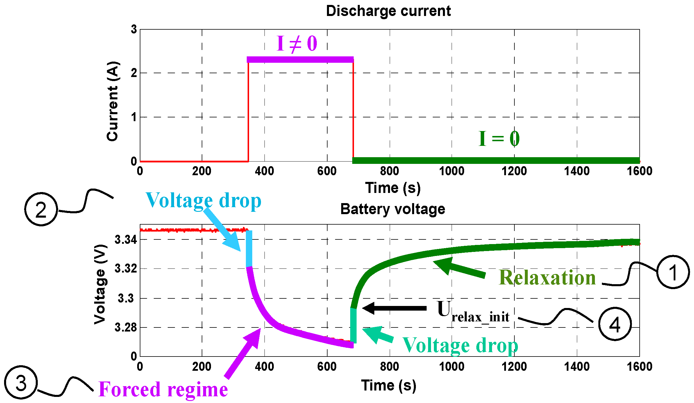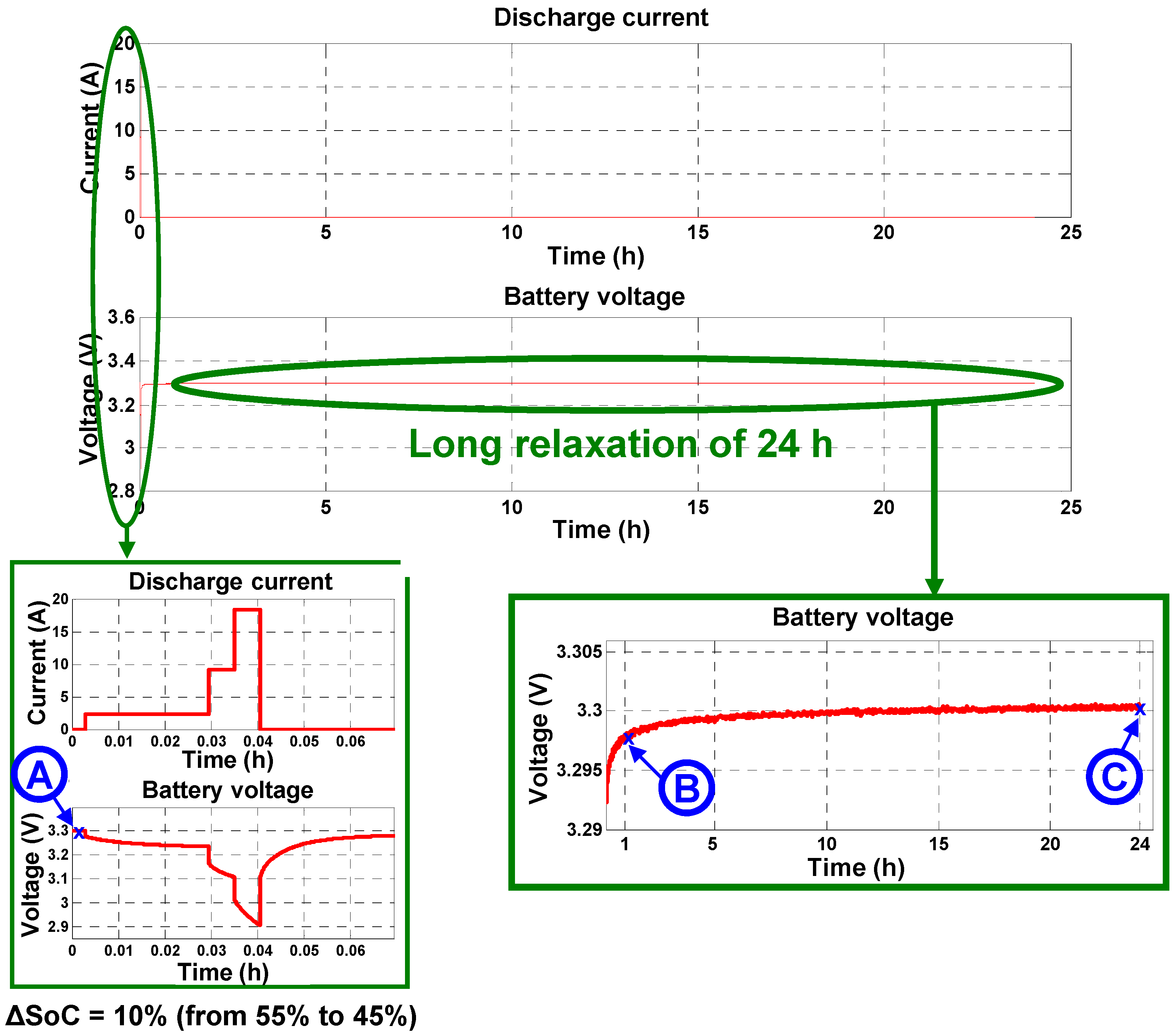For example, Figure 1 shows the typical voltage response of a battery following a discharge current pulse. The relaxation corresponds to the phase after a period of discharge, during which there is no current and the battery voltage tends towards a steady state.

The voltage measured at the end of the relaxation can be considered as the OCV value at this SoC. Figure 1 also shows two other phases of the battery voltage. One is the phase of voltage drop, which occurs when the current level changes. Another one is the phase of forced regime during which the battery current is not zero.

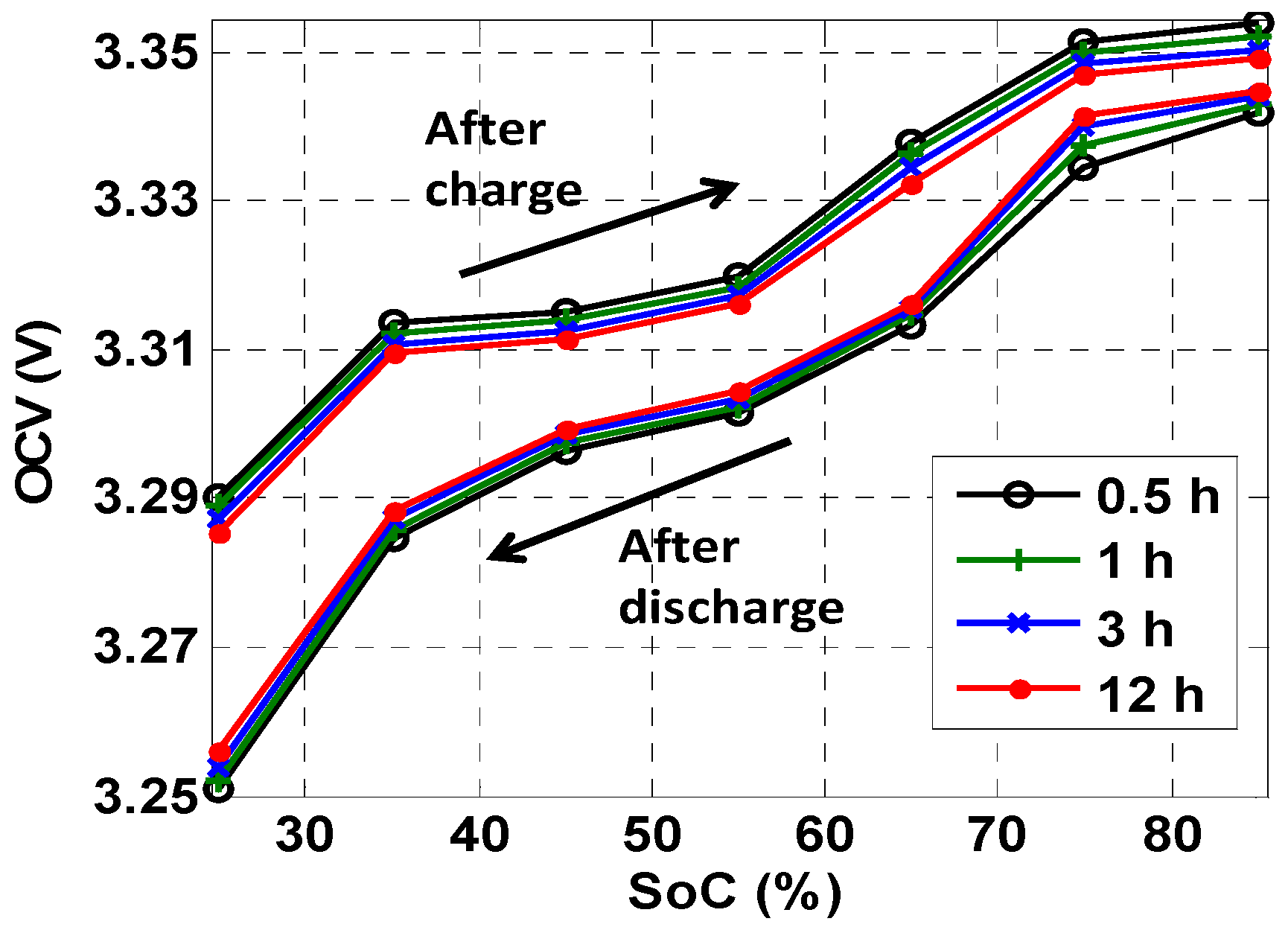
Relaxation time has a significant impact on the measured voltage, which is considered to be the OCV at the end of relaxation. Figure 2 shows the measurement results of OCV at different SoCs and after different relaxation times of a Li-ion battery. The curves measured after discharge and charge are different. The presence of gaps between the two curves is called hysteresis. When the relaxation time increases, the value of relaxation voltage measured in discharge increases and the one in charge decreases. The longer the relaxation time, the more the measurement of the battery voltage is close to the real OCV. In fact, the battery voltage still evolves beyond a few hours. In [1], it was stated that it may take over 24 h before the battery voltage stabilizes.

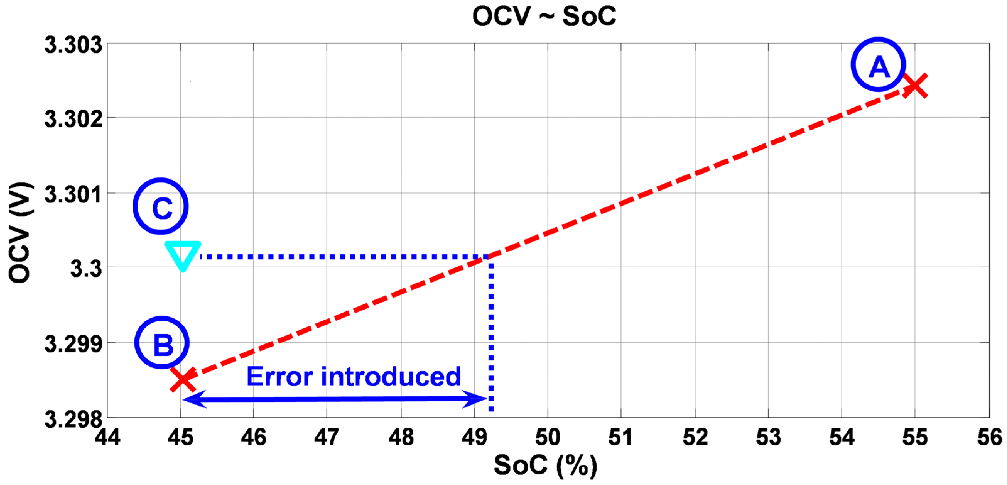
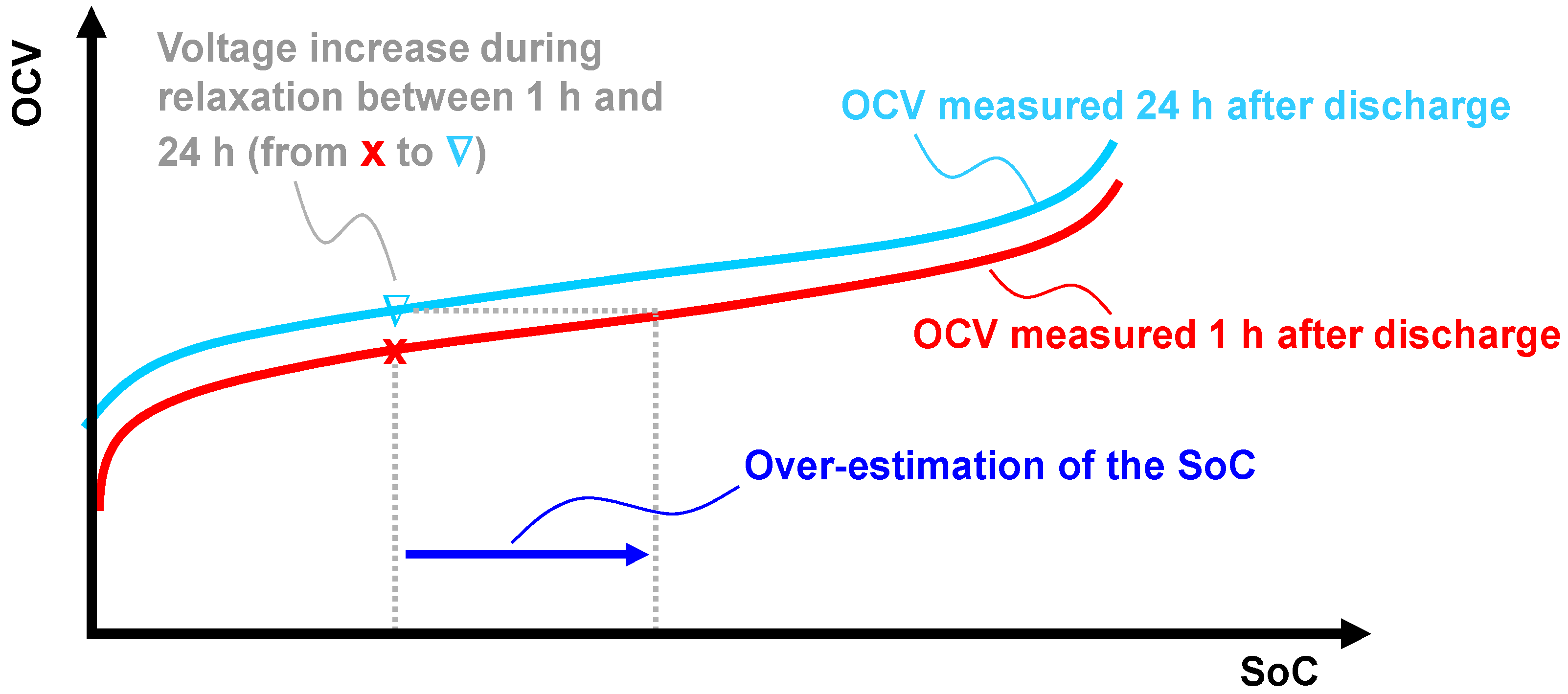
If the voltage variation during the relaxation is not taken into account in OCV estimation, error will be introduced into the estimation of SoC from the voltage. For example, as shown in Figure 3, if the OCV-SoC curve approximated from the voltage measured after 1 h is used as the reference for estimating the SoC from the voltage measurement, the voltage increase during relaxation after discharge between 1 h and 24 h will introduce an overestimation of the SoC.

The characterization of the voltage change during long relaxation (e.g., 24 h) requires a long testing time. As the relaxation is dependent on the SoC, the measurements must be repeated at different SoCs. Yet, such extensive testing would put a heavy load on testing planning, and increase the testing costs. It is therefore interesting to reduce or adapt the measurement time of relaxation to the necessary desired precision. However, with a reduced measurement time, long-term change in voltage cannot be observed. The problem to solve is to reduce the measurement time of relaxation while maintaining the accuracy of the voltage final value.

In the literature, the problem of reducing the measurement time of relaxation has seldom been addressed. In [2], a method of rapid testing was proposed for getting the OCV-SoC curve. However, slow variation of the voltage during the relaxation phase is not fully taken into consideration in this method. Several extrapolation methods of the battery relaxation voltage are proposed in two patents and one paper: Patents [3,4] used an analytical relaxation law to estimate the OCV and SoC of the battery when the battery is not in steady state. Reference [5] used an original equivalent circuit model of relaxation with parameters varying over time. However, all these proposed methods do not use conventional electrical circuits and may be problematic for embedded implementation. In [6], a fast extrapolation method is proposed to estimate OCV-SoC by using 6 min of relaxation; however, the error of estimation is still 4 mV apart from the OCV obtained from 5 h of relaxation. In [7], a similar method was used with 10 min of relaxation with an error of the order of 5 mV. As we could see further in this paper, an error of 2 mV in OCV-SoC curve could cause an important error in SoC estimation.

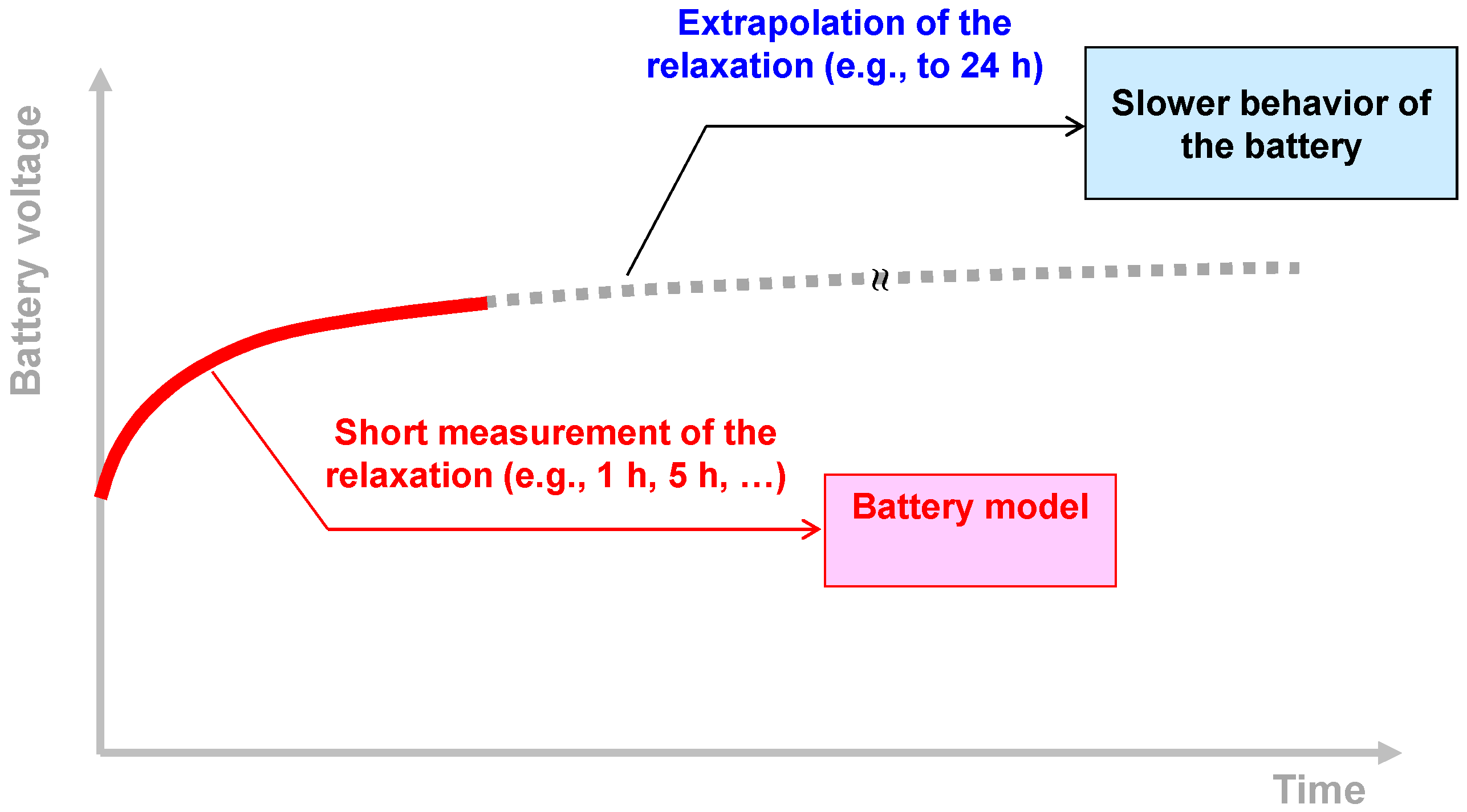
In this paper, a new method to characterize long relaxation voltage is proposed with an error of about 1 mV. This method uses the extrapolation of conventional electric circuit response and takes into consideration the slow voltage variation during relaxation. The principle of the method, illustrated in Figure 4, comprises: (i) a full relaxation measurement (e.g., 24 h) for a single SoC to calibrate the method; (ii) several shorter relaxations (e.g., 1 h, 5 h) measured at various considered SoCs; and (iii) an extrapolation to a longer duration (the same as in i) for each previous measurement.

This paper is organized as follows. Section 2 gives a mathematical description of relaxation by using an electrical model. Section 3 describes a study of the long relaxation, which reveals the possibility of extrapolating the slow voltage behavior of the relaxation from a short and partial measurement. Section 4 gives details on the proposed extrapolation method. The validation of the proposed method through both simulations and experiments is discussed in Section 5; Section 6 concludes the paper.

2. Mathematical Description of Relaxation

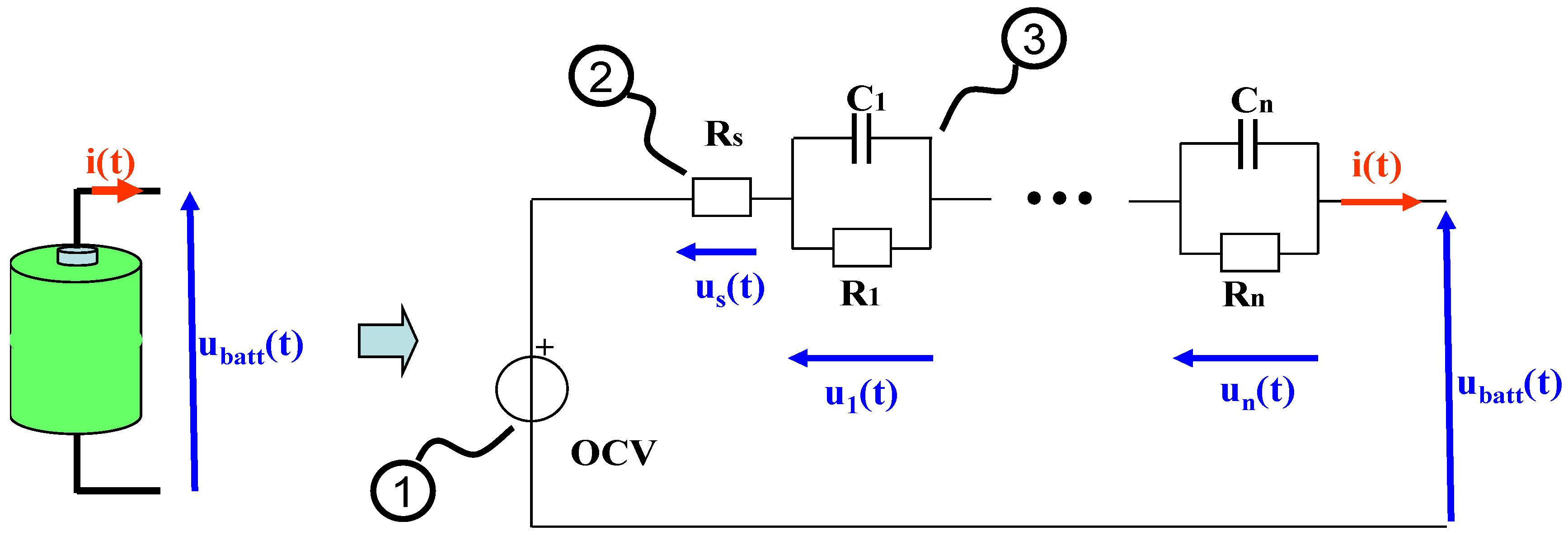
Several types of models can be used to represent the temporal behavior of the battery (e.g., electrochemical models [8], equivalent circuit model [9,10], black box model [11]. In this paper, an equivalent circuit model is chosen to study the relaxation because it is simple, fast, robust, with a good compromise of accuracy/simplicity, suitable for the application of electrified vehicles, and is easily integrated into simulation software. The model used to represent the dynamic behavior of the battery is shown in Figure 5. This model is composed of: (1) a voltage source to represent the OCV to a given SoC; (2) a resistance R_s to represent the voltage drop; and (3) several R_i//C_i circuits in series to represent the forced regime and relaxation. All these parameters of the model are mainly dependent on the SoC, the temperature, the current (amplitude and direction), and the aging.

During the relaxation phase, as the current is zero, the voltage drop across the resistance R_s is zero. However, voltage in individual R_i//C_i circuits is still dependent on time. By denoting U_{i_Relax} the voltage drop on R_i//C_i at the beginning of relaxation, the voltage of the battery during relaxation can be expressed by:

$$u_{\text{batt}}(t)=U_{\text{Relax\_init}}+{\displaystyle \sum _{i=1}^n{U}_{i\text{\_Relax}}\cdot \left(1-{\mathrm{e}}^{-\frac{t-t_0}{{\mathsf{\tau }}_{i\text{\_Relax}}}}\right)}$$

(1)

where U_{Relax_init} is the initial battery voltage at the beginning of relaxation (see (4) in Figure 1) which can be measured directly; t₀ is the moment when the relaxation starts; and τ_{i_Relax} is the time constant of R_i//C_i circuit during relaxation with τ_{1_Relax} < τ_{2_Relax} < ··· < τ_{n_Relax}.

The OCV expression is given by:

$$\text{OCV}=U_{\text{Relax\_init}}+{\displaystyle \sum _{i=1}^n{U}_{i\text{\_Relax}}}$$

(2)

Finally, the unknown parameters to be identified for a relaxation are the number of R_i//C_i (n), the voltage drops on each circuit R_i//C_i at the beginning of relaxation (U_{i_Relax}), and the time constant of each circuit R_i//C_i during relaxation (τ_{i_Relax}).

In this work, the parameters of the model depend only on the SoC. All experiments presented in this paper were realized at an ambient temperature of 25 °C and with new cells.

The structure of the model in Figure 5 is valid for both forced regime and relaxation phase. However, the values of parameters are different in each phase. The work of this paper focuses only on the relaxation phase.

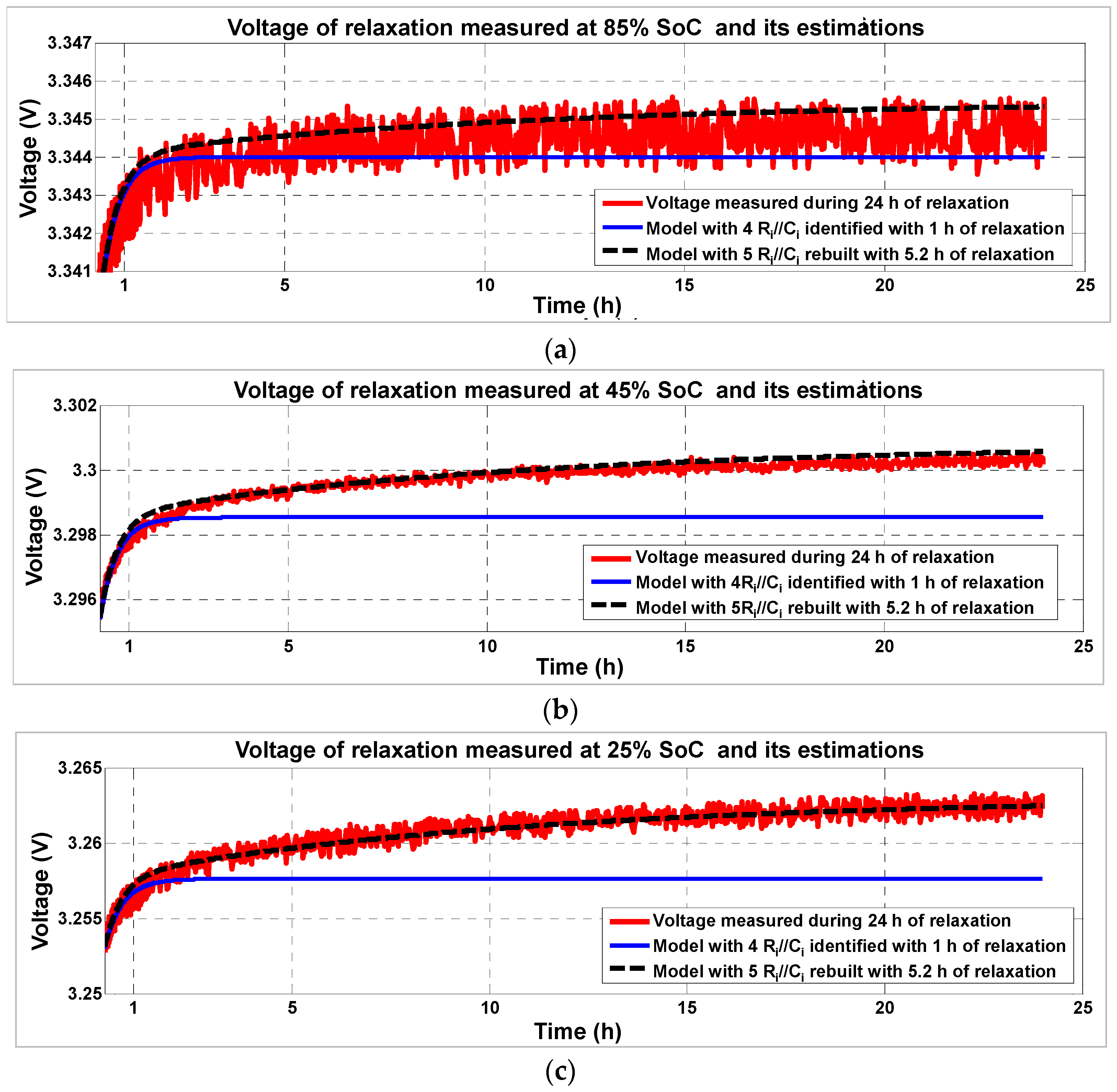
3. Study of a Long Relaxation

3.1. Test of a Long Relaxation

A relaxation experiment was carried out on an A123 26650 LiFePO₄ cell whose full capacity, nominal voltage, and cutoff voltage are 2.3 Ah, 3.3 V, and 2 V, respectively [12]. The cell was previously charged to 100% SoC through the method of constant current/constant voltage, and was discharged to 55% SoC by a constant current (1C). After 1 h of rest, a current profile was applied to discharge the cell from 55% SoC to 45% SoC. Then, a rest period of 24 h was imposed to measure the voltage evolution during relaxation, as shown in Figure 6. The cell was placed in a thermal chamber with ambient temperature regulated to 25 °C during all experiments. The minimum sampling time used for relaxation is 0.1 s.

Figure 6 shows that the voltage during relaxation evolves over several hours. The variation of voltage beyond 1 h appears negligible when compared to the battery voltage. Indeed, the voltage variation during relaxation between 1 h and 24 h is approximately 2 mV (between points B and C in Figure 6). Despite this small change, its determination is important for batteries with flat OCV-SoC curves because a difference of only a few millivolts may cause a significant error in SoC estimation. This applies to the tested cell, whose OCV-SoC curve has a substantially horizontal part between 40% SoC and 60% SoC. Figure 7 provides the SoC estimation error introduced by a difference of 2 mV for the case of Figure 6. Points A, B, and C in Figure 7 correspond to those in Figure 6. Points A and B correspond, respectively, to the OCVs of 55% and 45% SoC measured at 1 h after the discharge; point C corresponds to the OCV of 45% SoC measured at 24 h after discharge. If the OCV-SoC curve measured at 1 h after discharge is used as the reference to estimate the SoC from a voltage measurement, the voltage evolution during relaxation between 1 h and 24 h at 45% SoC (from Point B to Point C) will introduce an error of about 4% into the SoC estimation.

3.2. Identification of the Relaxation

This section presents the results of two identifications of the relaxation voltage shown in Figure 6. These results reveal the possibility of extrapolating the slow voltage behavior of the relaxation from a short and partial measurement.

The first identification is to identify the parameters of a model with four R_i//C_i circuits (n = 4 in Equation (1)) by using the first hour of relaxation voltage. The second identification is to identify the parameters of a model with five R_i//C_i circuits (n = 5 in Equation (1)) by using the voltage during 24 h of relaxation.

The use of models with four and five circuits R_i//C_i, respectively, for the first hour and for the 24 h of relaxation is a compromise between model complexity and identification accuracy. In the literature, many authors use two or three R_i//C_i circuits for the model [10,13,14,15]. However, these models are not intended to accurately represent at the same time the fast behavior related to charge transfer and the slow behavior related to diffusion effect (e.g., during relaxation). As we can see in Figure 8, which represents the root mean square (RMS) error for the estimation of the 24 h relaxation voltage versus the number of circuits for different battery technologies, the use of five R_i//C_i circuits allows us to obtain an error reading of less than 1%.

Identification of unknown parameters in Equation (1) is carried out with the least squares algorithm implemented in Matlab. The identification results are shown in Figure 9.

For the results of time constants (τ_{i_Relax}), the difference between the two models lies mainly in the last time constants, as highlighted in Figure 9. The first three time constants of the two models are of the same order of value. This implies that, when the relaxation time is longer, R_i//C_i circuits with greater time constants need to be added to the model in order to represent the slow dynamics of relaxation voltage with good accuracy. Figure 10 presents the simulation of voltage during a relaxation phase of 24 h by using the two models in Figure 9. The model with four R_i//C_i circuits is insufficient to adequately represent the entire relaxation due to the lack of a time constant with higher value.

For the results of the voltage drops (U_{i_Relax}) in Figure 9, U_{4_Relax} and U_{5_Relax} are much smaller than other U_{i_Relax}. In

Table 1. Comparison of the U_{i_Relax} for the two models.

Models	U1_Relax (mV)	U2_Relax (mV)	U3_Relax (mV)	U4_Relax (mV)	U5_Relax (mV)	${\displaystyle \mathbf{\sum }_{\mathit{i}\mathbf{=}\mathbf{1}}^{\mathbf{5}}{\mathit{U}}_{\mathit{i}\mathbf{\text{\_Relax}}}}$ (mV)
Model with four Ri//Ci	30.8	134.7	31.6	5.7	0	202.8
Model with five Ri//Ci	30.7	135.2	32.3	5.0	1.2	204.4
Difference (mV)	−0.1	0.5	0.7	−0.7	1.2	1.6

, a comparison between the values of U_{i_Relax} of the two models shows that there is a difference of 1.6 mV between the sums of U_{i_Relax}, which leads to a difference of 1.6 mV in the estimation of OCV according to Equation (2) for the two models. The difference is not only related to the value of U_{5_Relax} which is 1.2 mV, but also related to other U_{i_Relax}. This difference of 1.6 mV results in a voltage difference at the end of 24 h between the measured voltage and the estimated one using the model with four R_i//C_i circuits. If this difference in voltage could be estimated, it would be possible to reduce the length of the experiment.

3.3. Extrapolation of the Relaxation

This difference in voltage can be estimated by using a technique that transforms the voltage measurement from a linear-based time scale to a logarithmic time scale. Figure 11 shows such a transformation of the measured voltage for the relaxation of 24 h. The voltage estimated by the model with four R_i//C_i is also shown in the same figure. In Figure 11a, the divergence between the measured voltage and the estimated one starts at around 2.2 h, which corresponds to the end of the validity of the fourth time constant (τ_{4_Relax}) of the model with four R_i//C_i. The end of the validity, denoted as ∆t_val, is equal to five times the value of τ_{4_Relax} because after a time equal to 5τ_{4_Relax}, the influence of this time constant is considered negligible as e⁻⁵ = 0.7%. The voltage difference at the end of 24 h (denoted by ΔU_Diff in Figure 11a) between the measured and the estimated voltage is the one we want to estimate. In Figure 11b, with time in a logarithmic scale, the measured voltage beyond 2.2 h is close to a straight line, as indicated by the black dotted line. The voltage difference at the end of 24 h between the straight line and the estimated voltage of the model with four R_i//C_i can thus be used to estimate ΔU_Diff. The slope of the line could be determined by a linear regression using only a small part of the measured voltage beyond 2.2 h, as indicated in Figure 11b. The only problem to solve is to determine the added duration needed beyond 2.2 h to identify the line, as shown in Figure 11b. The advantage of the logarithmic scale is to enable estimation of this added duration needed. Indeed, as the objective is to estimate the value of ∆U_Diff between the four R_i//C_i model’s response after 24 h and the real measures, the linear shape of signals in the logarithmic scale (Figure 11b) is better than in the linear scale (Figure 11a), as explained in the following part of the text.

In short, the study of relaxation in this section reveals the possibility of extrapolating the slow behavior of the relaxation by using the observation that some part of the relaxation voltage is close to a straight line in logarithmic time scale, as shown in Figure 11. Based on the result of this study, an extrapolation method is elaborated. The method allows us to reconstruct a new model with five R_i//C_i from a short and partial measurement of relaxation voltage. The new model is capable of correctly estimating the slow relaxation voltage to 24 h. With this method, it is then possible to reduce the relaxation measurement to a shorter duration. The details of this method are discussed in the next section.

4. Extrapolation Method of Relaxation

4.1. Principle of the Method

The proposed method allows the characterization of the long relaxation battery voltage at different SoCs with a reduced time. For the sake of simplicity and practicality, the characterization for the relaxation of 24 h is taken as an example to explain the method. Furthermore, 24 h of relaxation is well adapted to automotive applications, where daily uses are regular. However, the method can be transposed to characterize relaxation with longer or shorter duration. The relaxation time can vary greatly with different technologies of cells and with the temperature of operation. The method includes two phases:

The first phase is to measure the battery voltage during 24 h of relaxation at an intermediate SoC (e.g., 45% SoC). With this measurement, a minimum duration (∆t_min, less than 24 h) is determined to measure the relaxation at other SoCs.

The second phase is to measure at other SoCs the battery relaxation voltage during the minimum duration defined in Step 1. With these measurements, a model with five R_i//C_i can be reconstructed. For each SoC tested, the parameters (U_{i_Relax} and τ_{i_Relax}) of the first four R_i//C_i are identified by using the measurement during the first hour of relaxation, like the example shown in Figure 9. The parameters (U_{5_Relax} and τ_{5_Relax}) of the fifth R//C circuit (R₅//C₅) can be estimated by using the relaxation voltage measured after the first hour and the extrapolation at 24 h of the signal measured during ∆t_min.

Once the values of U_{i_Relax} and τ_{i_Relax} are obtained, OCV can be calculated from the measurement of U_{Relax_init} and Equation (2).

The determinations of the minimum duration in the first phase and the five R_i//C_i in the second phase are detailed as follows.

4.2. Determination of the Minimum Duration

The minimum duration ∆t_min is calculated as:

Δt_min = Δt_val + Δt_added

(3)

where ∆t_val is the end of the validity of the fourth time constant (τ_{4_Relax}) of the model with four R_i//C_i. τ_{4_Relax} and other parameters of the model with four R_i//C_i are determined by using the first hour of relaxation. ∆t_added is the added duration needed to identify the slope of the line, as in Figure 11b. To determine the added duration needed just to identify the slope, a study is needed on the relationship between the measurement duration added beyond ∆t_val and the identification accuracy of the line slope. The study is conducted in several steps, as illustrated in Figure 12 by using the data in Figure 11.

To overcome the influence of measurement noise on the voltage, the model with five R_i//C_i identified with relaxation of 24 h was used (green curve in Figure 12).

After transforming the time into a logarithmic scale, an added duration beyond ∆t_val (2.2 h in the example of Figure 12) is used to identify the slope of the line. The error ΔU_Error at the end of 24 h between the identified line and the estimation of the model with five R_i//C_i is used to assess the accuracy of the identified line slope.

By repeating the calculation of the error ΔU_Error with different added durations, the evolution of the error versus the added duration can be obtained.

Figure 13 shows the evolution of the error vs. the value of the added duration for the relaxation of Figure 12. In Figure 13, the error ∆U_Error decreases as the added duration increases. By choosing an acceptable value of the error, the necessary duration of ∆t_added can be determined. For example, to achieve a level of precision equal to 0.5 mV, the duration added is equal to 3 h. In this case, the minimum duration ∆t_min is equal to 5.2 h (2.2 h + 3 h) according to Equation (3). This means that for the relaxation at other SoCs, only 5.2 h of measurement is needed instead of 24 h.

4.3. Determination of the Parameters in R₅//C₅

Two unknown parameters (τ_{5_Relax} and U_{5_Relax}) of the five R_i//C_i circuit need to be identified for every relaxation measured with the minimum duration. The time constant τ_{5_Relax} is equal to the one identified in the first phase with 24 h of relaxation. τ_{5_Relax} is supposed to be constant for all other SoCs. This was verified by the tests described as follows for different battery technologies. The same tests of relaxations of 24 h as in Section 3 were performed on three different cells (LiFePO₄, NMC, and NiMH cells) at different SoCs. While comparing the values of the time constants identified for the model with five R_i//C_i, a logarithmic distribution of time constants was found for the three cells. Figure 14, Figure 15 and Figure 16 present the results of the time constants identified for the model with five R_i//C_i. The results show that the distribution of τ_{i_Relax} in a logarithmic scale is substantially linear. The time constants τ_{i_Relax} for different SoCs and different cells also have the same magnitudes of value for the same index of i. For example, the values of τ_{5_Relax} for different SoCs and different cells are very close (around 38,000 s). The magnitudes of values of different time constants are: τ_{1_Relax} = 1.3 s, τ_{2_Relax} = 17 s, τ_{3_Relax} = 220 s, τ_{4_Relax} = 2900 s and τ_{5_Relax} = 38,000 s (≈11 h).

Another unknown parameter U_{5_Relax} of the five R_i//C_i circuit is calculated by the following expression:

$$U_{\text{5\_Relax}}=\frac{\mathrm{\Delta }{U}_{\text{Diff}}^{\prime }}{\left(1-{\mathrm{e}}^{-\frac{\mathsf{\Delta }{t}_{\text{Relax}}}{{\mathsf{\tau }}_{\text{5\_Relax}}}}\right)}$$

(4)

where ∆t_Relax is the total duration of the relaxation (here 24 h) and ∆U′_Diff is the estimated value for ∆U_Diff (Figure 11). In the second phase, the voltage measured during relaxation for every SoC is limited to the minimum duration, which is determined previously in the first phase (e.g., 5.2 h). The first hour of the measurement is used to identify the parameters of the model with four R_i//C_i. The measurement after the end of the validity of the fourth time constant (∆t_val) is used to identify a line in logarithmic scale, as illustrated in Figure 12. ∆U′_Diff is equal to the voltage difference at the end of 24 h between the estimation of the model with four R_i//C_i and the identified line. At this point, the interest of the linear shape of the curve is obvious as it facilitates the computation of ∆U′_Diff and finally of U_{5_Relax}.

4.4. Discussion on the Values of U_{i_Relax}

The values of U_{i_Relax} for the A123 cell at different values of SoC are given in

Table 2. Values of U_{i_Relax} for the A123 cell at different values of SoC.

SoC	U1_Relax (mV)	U2_Relax (mV)	U3_Relax (mV)	U4_Relax (mV)	U5_Relax (mV)	ΣUi_Relax (mV)
85%	24.7	116.7	29.9	9.1	1.5	181.9
45%	30.8	134.7	31.6	5.7	2.3	205.0
25%	34.6	134.4	39.6	8.1	5.4	222.1

. It can be seen that U_{i_Relax} varies when SoC goes from 25 to 85. Consequently, the same set of U_{i_Relax} values cannot be used for all SoCs. If the same set of values was used to estimate the relaxation voltage for all SoCs, an important error in voltage estimation would be generated at the end of 24 h. For example, from Table 2, if values of 45% SoC are used, the error in the voltage estimation would be 205.0 mV − 181.9 mV = 23.1 mV for 85% SoC and 222.1 mV − 205.0 mV = 17.1 mV for 25% SoC. As mentioned in Figure 7, such an error in voltage may generate an important error in the estimation of SoC.

5. Validation Test

To evaluate the performance of the proposed method, a validation test was performed by using three relaxations of 24 h measured on the A123 cell. First, with the relaxation of 24 h at SoC of 45% (Figure 11) and by choosing 0.5 mV as the acceptable accuracy, the minimum measurement duration (∆t_min) is determined to be 5.2 h (Figure 13). Second, with the measurements of the first 5.2 h of relaxation at SoC of 85%, 45%, and 25%, three models with five R_i//C_i were reconstructed. The performance of the reconstructed models to estimate relaxations of 24 h is shown in Figure 17. The errors at the end of 24 h between the estimation of the reconstructed model and the measurement are −0.8 mV at SoC 85%, −0.2 mV at SoC 45% and 0.1 mV at SoC 25%. The result shows that the reconstructed models can accurately estimate the long relaxation during 24 h. Thus, to obtain the relaxations of 24 h at these three SoCs with the proposed method, it is only necessary to perform a measurement of 24 h of relaxation at 45% SoC and two measurements of 5.2 h at 85% and 25% SoC, in total 34.4 h of measurement. Compared to the conventional method, which requires 72 h of measurement (e.g., three measurements of 24 h for the three SoCs), the proposed method saves 37.6 h, which represents a gain of 52% in measurement time, without considering the setting of initial SoC for each test.

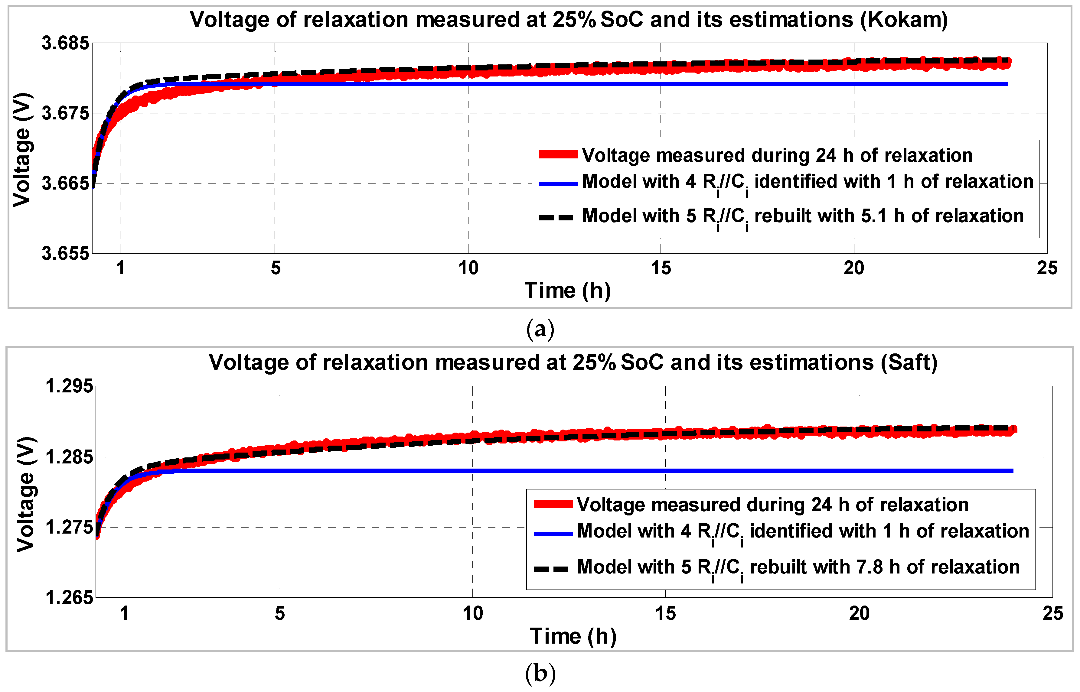
Validation tests were also conducted on two other technologies (NMC and NiMH). For example, Figure 18 presents the result for estimation of relaxation voltage at 25% SoC for the two cells. By using the same acceptable accuracy as the A123 cell (0.5 mV), the minimum measurement duration (∆t_min) is determined to be 5.1 h for the Kokam cell and 7.8 h for the Saft cell. The accurate estimation result in Figure 18 shows that the proposed method is also applicable to these two technologies.

6. Conclusions

A fast characterization method to determine the full relaxation response of a battery (e.g., 24 h) has been proposed in this paper. This method allows for reconstructing an electric circuit model that is capable of correctly estimating the voltage relaxation. Only one complete measurement of the voltage relaxation at one SoC is needed to calibrate the method. For other SoCs, only a shorter measurement duration (e.g., about 5 h) is necessary. When compared with a step-by-step charging and discharging protocol (ΔSoC = 5% with 3 h of rest at each step) to determine the OCV (SoC) curve like in [1], the present method has the following advantages: besides giving the OCV (SoC) curve it enables us to compute the variation of the output voltage during relaxation. Furthermore, if one wants to estimate 24 h of relaxation with a step-by-step protocol, it could last 40 × 24 h (20 SoC levels during charging and 20 SOC levels during discharging), which represents 40 days of experiments. With our method, only one measurement of 24 h is necessary plus 40 measurements of 5 h, which represents only nine days of works. This method could save a lot of characterization time, which is very useful when tests are required at different temperatures and aging states. When the method is applied for relaxation after charge and discharge, the OCVs obtained could also bring out the hysteresis. Furthermore, it is generic so it could easily be extended to any technology of battery and adapted to longer or shorter relaxation durations.

This method could be applied to calculate the SoC of batteries in EVs from measurements of OCV. In that case, the curve OCV (SoC) stored in the on-board computer and used to calculate the SoC is usually determined after a specified relaxation time (e.g., 24 h). The proposed model of relaxation voltage can be used to accurately predict the OCV and thus the SoC at the specified time without waiting for it. On the other hand, when the curve OCV (SoC) stored in the on-board computer is determined after a short relaxation time (e.g., 1 h), the proposed model of relaxation voltage can be used to go back in time. For example, when the vehicle has been parked for a longer time (e.g., 24 h), the value of OCV at 1 h, and thus the SoC can be determined from the measured value of OCV at 24 h.

References

1. Roscher, M.A.; Sauer, D.U. Dynamic electric behavior and open-circuit-voltage modeling of LiFePO4-based lithium ion secondary batteries. J. Power Sources 2011, 196, 331–336. [Google Scholar] [CrossRef]
2. Abu-Sharkh, S.; Doerffel, D. Rapid test and non-linear model characterization of solid-state lithium-ion batteries. J. Power Sources 2004, 130, 266–274. [Google Scholar] [CrossRef]
3. Bergveld, H.; Pop, V.; Notten, P.H.L. Apparatus and Method for Determination of the State of Charge of a Battery When the Battery Is Not in Equilibrium. U.S. Patent 20100036627 A1, 11 February 2010. [Google Scholar]
4. Driemeyer-Franco, A.; Lucea, M.; Saint-Marcoux, A.; Bui-Van, A.-L.; Perichon, P. Système et Procédé Correspondant D’estimation de L’état de Charge d’une Batterie. Patent WO 2013171425 A1, 21 November 2013. (In French)[Google Scholar]
5. Pei, L.; Wang, T.; Lu, R.; Zhu, C. Development of a voltage relaxation model for rapid open-circuit voltage prediction in lithium-ion batteries. J. Power Sources 2014, 253, 412–418. [Google Scholar] [CrossRef]
6. Petzl, M.; Danzer, M.A. Advancements in OCV measurement and analysis for lithium-ion batteries. IEEE Trans. Energy Convers. 2013, 28, 675–681. [Google Scholar] [CrossRef]
7. Baronti, F.; Zamboni, W.; Roncella, R.; Saletti, R.; Spagnuolo, G. Open-Circuit Voltage Measurement of Lithium-Iron-Phosphate Batteries. In Proceedings of the IEEE Instrumentation and Measurement Technology Conference (I2MTC), Taipei, Taiwan, 23–26 May 2015; pp. 1711–1716.
8. Chaturvedi, N.A.; Klein, R.; Christensen, J.; Ahmed, J.; Kojic, A. Algorithms for advanced battery-management systems. IEEE Control Syst. Mag. 2010, 30, 49–68. [Google Scholar] [CrossRef]
9. Urbain, M.; Hinaje, M.; Raël, S.; Davat, B.; Desprez, P. Energetical modeling of lithium ion batteries including electrode porosity effects. IEEE Trans. Energy Convers. 2010, 25, 862–872. [Google Scholar] [CrossRef]
10. Chen, M.; Rincon-Mora, G.A. Accurate Electrical Battery Model Capable of predicting runtime and I-V performance. IEEE Trans. Energy Convers. 2006, 21, 504–511. [Google Scholar] [CrossRef]
11. Sarvi, M.; Masoum, M.A.S. A Neural Network Model for Ni-Cd Batteries. In Proceedings of the 43rd International Universities Power Engineering Conference (UPEC), Padova, Italy, 1–4 September 2008; pp. 1–5.
12. A123 Systems. Li-Ion 26650 Cylindrical Cell, 2011. Available online: http://www.a123systems.com (accessed on 14 May 2011).
13. Zhang, J.; Ci, S.; Sharif, H.; Alahmad, M. Modeling discharge behavior of multicell battery. IEEE Trans. Energy Convers. 2010, 25, 1133–1141. [Google Scholar] [CrossRef]
14. Kroeze, R.; Krein, P.T. Electrical Battery Model for Use in Dynamic Electric Vehicle Simulation. In Proceedings of the IEEE Power Electronics Specialists Conference, Rhodes, Greece, 15–19 June 2008; pp. 1336–1342.
15. Hu, Y.; Yurkovich, S.; Guezennec, Y.; Yurkovich, B.J. Electro-thermal battery model identification for automotive applications. J. Power Sources 2011, 196, 449–457. [Google Scholar] [CrossRef]
16. Kokam. Li-Ion SLB603870H Cell, 2011. Available online: http://www.kokam.com (accessed on 14 May 2011).
17. Saft. NiMH VHCS3500 Cell, 2011. Available online: http://www.saftbatteries.com (accessed on 14 May 2011).
Figure 1. Voltage response of a battery after discharge.
Batteries 02 00007 g001
Figure 2. Open circuit voltage (OCV)-state of charge (SoC) curves of a Li-ion battery LiFePO4 technology obtained after different relaxation times.
Batteries 02 00007 g002
Figure 3. Illustration of the overestimation of SoC caused by long relaxation.
Batteries 02 00007 g003
Figure 4. Principle of the proposed method.
Batteries 02 00007 g004
Figure 5. Thevenin model.
Batteries 02 00007 g005
Figure 6. Voltage measurement during a relaxation period of 24 h at 45% SoC for an A123 cell.
Batteries 02 00007 g006
Figure 7. SoC estimation error introduced by voltage evolution during relaxation on the cell of Figure 6.
Batteries 02 00007 g007
Figure 8. Average root mean square (RMS) error for the estimation of the 24 h relaxation voltage vs. the number of Ri//Ci circuits for A123 2.3 Ah LiFePO4 cell, Kokam 1.5 Ah nickel manganese cobalt (NMC) cell [16], and Saft 3 Ah nickel metal hydride (NiMH) cell [17].
Batteries 02 00007 g008
Figure 9. Results of identifications.
Batteries 02 00007 g009
Figure 10. Simulation of the voltage during 24 h of relaxation with the two model parameters in Figure 9.
Batteries 02 00007 g010
Figure 11. Long relaxation (24 h) at 45% SoC of an A123 cell with: (a) linear scale on time axis and (b) a logarithmic scale.
Batteries 02 00007 g011
Figure 12. Illustration of steps to investigate the relationship between the added duration beyond 2.2 h and the identification accuracy of the line slope.
Batteries 02 00007 g012
Figure 13. Error ∆UError vs. the added duration ∆tadded.
Batteries 02 00007 g013
Figure 14. Time constants τi_Relax identified of the model with five Ri//Ci for different SoCs of an A123 2.3 Ah LiFePO4 cell.
Batteries 02 00007 g014
Figure 15. Time constants τi_Relax identified of the model with five Ri//Ci for different SoCs of a Kokam 1.5 Ah NMC cell.
Batteries 02 00007 g015
Figure 16. Time constants τi_Relax identified of the model with five Ri//Ci for different SoCs of a Saft 3 Ah NiMH cell.
Batteries 02 00007 g016
Figure 17. Performance of the model with five Ri//Ci reconstructed with 5.2 h of relaxation at SoC of: (a) 85%; (b) 45%; and (c) 25% for A123 cell.
Batteries 02 00007 g017
Figure 18. Performance of the model with five Ri//Ci reconstructed at 25% SoC for: (a) a Kokam cell with 5.1 h of relaxation; and (b) a Saft cell with 7.8 h of relaxation.
Batteries 02 00007 g018