Article

Swift Prediction of Battery Performance: Applying Machine Learning Models on Microstructural Electrode Images for Lithium-Ion Batteries

Materials Research Institute Aalen (IMFAA), Aalen University, Beethovenstr. 1, 73430 Aalen, Germany
*
Authors to whom correspondence should be addressed.
Batteries 2024, 10(3), 99; https://doi.org/10.3390/batteries10030099
Submission received: 19 January 2024 / Revised: 4 March 2024 / Accepted: 8 March 2024 / Published: 12 March 2024

Abstract

:
In this study, we investigate the use of artificial neural networks as a potentially efficient method to determine the rate capability of electrodes for lithium-ion batteries with different porosities. The performance of a lithium-ion battery is, to a large extent, determined by the microstructure (i.e., layer thickness and porosity) of its electrodes. Tailoring the microstructure to a specific application is a crucial process in battery development. However, unravelling the complex correlations between microstructure and rate performance using either experiments or simulations is time-consuming and costly. Our approach provides a swift method for predicting the rate capability of battery electrodes by using machine learning on microstructural images of electrode cross-sections. We train multiple models in order to predict the specific capacity based on the batteries’ microstructure and investigate the decisive parts of the microstructure through the use of explainable artificial intelligence (XAI) methods. Our study shows that even comparably small neural network architectures are capable of providing state-of-the-art prediction results. In addition to this, our XAI studies demonstrate that the models are using understandable human features while ignoring present artefacts.

1. Introduction

Since their introduction into the market in 1991 [1], lithium-ion batteries have become one of the most important devices for electrochemical energy storage. They are widespread in many fields of application, from consumer electronics and power tools to large-scale stationary storage solutions for wind and solar energy and electric vehicles [2,3]. Lithium-ion batteries comprise thin electrodes (anode and cathode) that, in turn, consist of a metal foil current collector with a porous active mass coating. The active mass contains active material particles capable of storing and releasing lithium ions [4]. In addition to the chemical composition and crystal structure of the active materials used [5], the battery performance is, to a great extent, influenced by the rather complex microstructure of the active mass coating, i.e., the coating thickness, particle size distribution, porosity, and tortuosity, as well as the carbon binder domain distribution [6,7,8,9,10,11,12,13,14,15,16,17].
The influence of microstructural parameters on electrode performance has been investigated experimentally [7,8,12,14,18,19,20,21,22,23] and computationally [24,25,26,27,28,29,30,31,32]. Many studies focus on porosity and electrode thickness, as these two microstructural features are relatively easy to assess and highly relevant in terms of both electrode manufacturing and electrode performance. For example, Zheng et al. [7] and Kang et al. [19] experimentally examined the effects of calendaring on porosity, thickness and the resulting electrochemical characteristics of LiNi1/3Co1/3Mn1/3O2 (NCM111) cathodes. Zheng et al. [12] used electrodes with varying coating thickness and constant porosity, while Heubner et al. [14] provided a study that considered both porosity and electrode thickness. Chen et al. [13] used a combination of experiments and simulation with 1D/2D multi-physics finite model to assess the influence of porosity in an NCM cathode. The influence of electrode thickness on the rate performance of NCM cathodes was studied by Danner et al. [32] using a detailed 3D microstructural resolved simulation based on synchrotron X-ray radiation tomographies. To summarise these studies, the microstructure–performance correlations of electrodes are complex. However, as a general conclusion, it can be stated that thin electrodes with high porosities result in electrodes with a higher power density but lower energy density.
From the perspective of modelling and simulation, a variety of models are available, such as pseudo-2D models [29,30,31,33] or more complex 3D models [26,32,34,35,36], to study microstructure–performance correlations. However, in addition to computing capacities, these approaches require reliable input parameters such as lithium diffusion coefficients in active materials, electronic conductivity, or even 3D microstructural data of the electrodes [37,38], which, in turn, require sophisticated experiments [39]. In addition, such experiments are subject to certain uncertainties, which consequently also apply to the data. However, experimental studies, as described above, require a lot of time and cannot consider all parameter variations within the design of the experiment.
Modern machine learning algorithms have proven to be able to reveal complex input-output relations to solve difficult tasks. Algorithms outside the field of deep learning are able to extract and select relevant features from the given data and model them to solve a task. Those capabilities, together with the increasing availability of large quantities of high-quality data, enabled a wide range of applications [40] and made data-driven methods, especially machine learning, one of the fastest-growing topics in materials research. The applications of machine learning and deep learning in materials research include material analysis [41,42], material design [43], and process optimization [44].
Thus, machine learning-based models could provide a fast and robust tool for analysing electrode microstructures and predicting the electrochemical performance of an electrode. The use of ML in battery development and manufacturing is a relatively new approach [45,46,47]. The publications mainly consider the AI-assisted development and optimisation of active materials [48,49], or process and quality monitoring in electrode manufacturing [50,51,52], also using Data Mining [53]. Machine learning has already been used to extract features from electrode microstructures based on X-ray tomography data [54].
In our study, we applied an image regression model based on convolutional neural networks (CNNs). The advantage of this approach is that no conventional microstructural features, such as porosity, layer thickness, and particle size, are extracted by the model or need to be given to the model by the user. Instead, the model learns directly from the images using granular features without knowing the microstructural components and their actual function within the electrode [55,56]. In doing so, we also avoided pushing the model in a certain direction. Using explainable AI, we were able to observe if the model will be able to identify microstructural features which are physically sensible and are known to affect the rate performance, or if the model might predict microstructure–performance correlations that have not yet been discovered. To our knowledge, the use of 2D microstructural data of electrodes to directly predict electrode performance without feature segmentation and quantification has not yet been reported.
In this study, we present a novel approach and the feasibility of modern machine learning techniques as a powerful, fast, and cost-effective tool to predict the performance parameters of electrodes for lithium-ion batteries based on light microscopy images of 2D cross-sections. The proposed methods show a high potential as they are capable of assessing the performance and quality of electrodes with relatively easy-to-implement methods in the early stages of development and production.

2. Materials and Method

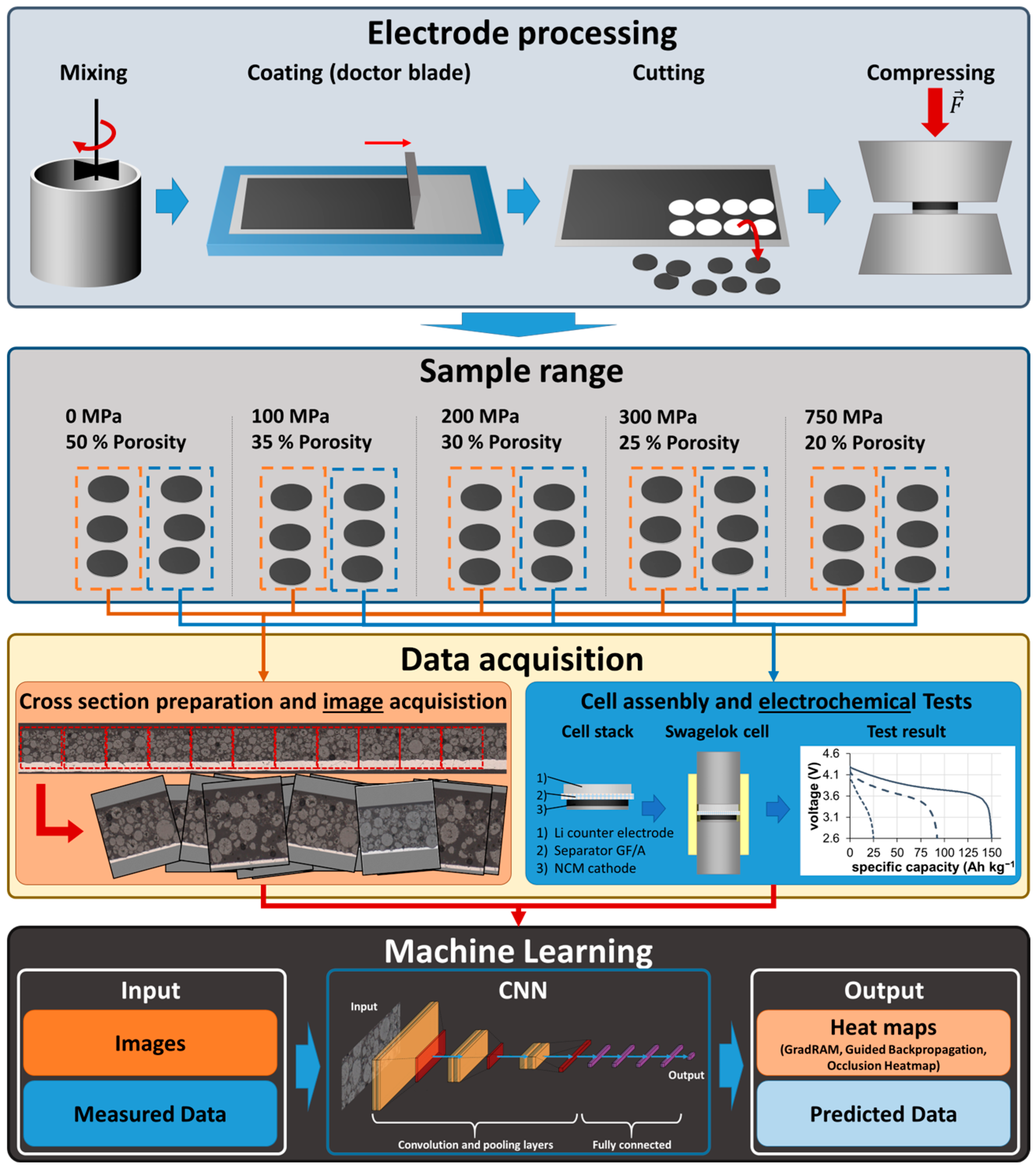
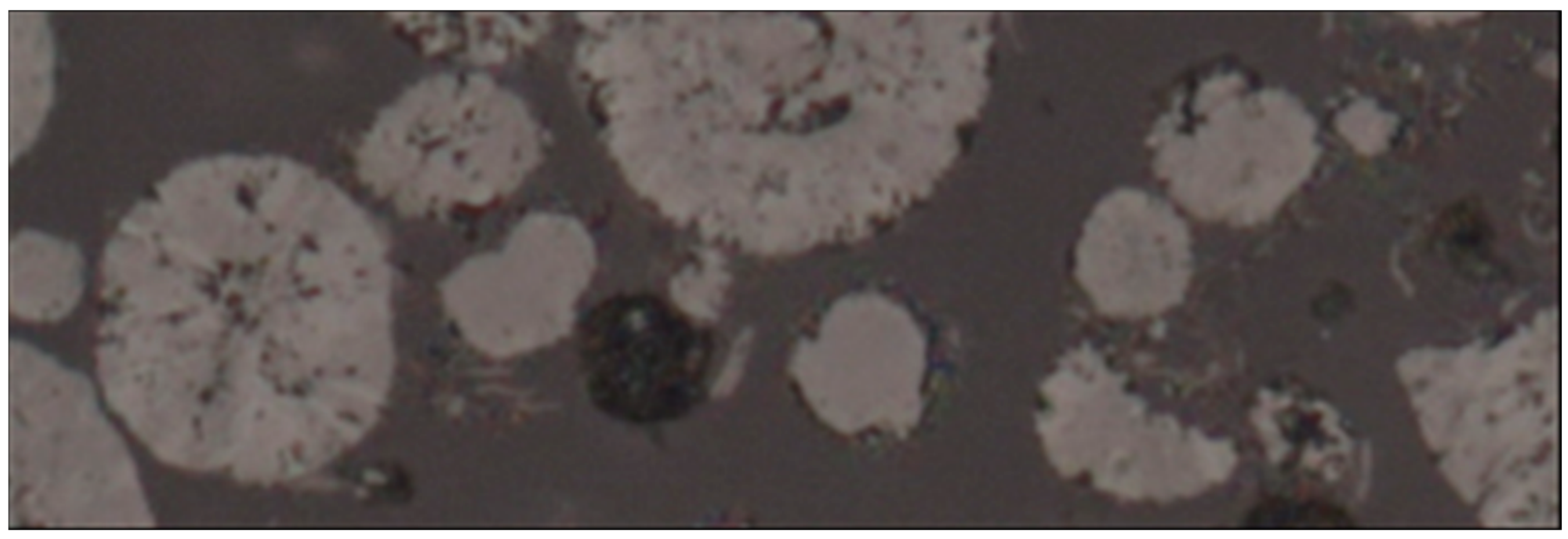
2.1. Sample Preparation, Electrochemical Tests and Image Data Acquisition

Figure 1 illustrates the methodical approach and process we followed in this study. Electrodes were prepared and densified with different uniaxial loads to simulate the calendaring process during electrode manufacturing. From these electrodes, cross-sectional images were acquired and Swagelok-type cells were prepared for electrochemical testing. The image data and data from the electrochemical rate tests were then used to train a machine learning model and predict the capacities for different electrode microstructures and C-rates.
The electrodes and electrochemical data we used in this study are presented in our previous work [8], which also includes a detailed description of the electrode manufacturing process and the methods used for electrochemical characterisation. The electrodes that were investigated consist of 92 wt% LiNi1/3Co1/3Mn1/3O2 (NCM111) as the active cathode active material, 4 wt% PvdF as the binder, and 4 wt% conductive additives coated on a 15 µm thick aluminium foil as the current collector. The coating was made by dissolving the components in N-Methyl-2-pyrrolidone (NMP) and coating the slurries with the aluminium current collector using the doctor blade method. After evaporating the solvent at room temperature, the active mass loading of the electrode sheet was 15.4 mg cm−2, corresponding to a theoretical areal capacity of 2.46 mAh cm−2. From the coated sheet, Ø10 mm electrodes were cut and compressed with a universal testing machine (RSA 100; Schenk), with uniaxial loads gradually increasing from 0 MPa to 750 Mpa, resulting in irreversible mechanical densification of the electrodes with porosities between 50% (uncompressed) and 20% (750 MPa). Table 1 shows the compression loads and the resulting porosities. Porosities are given as a reference and as an identifier for the samples.
The porosities of the electrodes ε were calculated using the bulk density of the active mass coating ρAM and the skeletal density ρS of the solid components. The first was determined by measuring the mass and thickness of the densified electrodes with a laboratory scale (AX324; Ohaus Europe GmbH, Nänikon, Switzerland) and a micrometre gauge (MarCator 1086R; Mahr GmbH, Göttingen, Germany). The mass of the current collector was subtracted. Skeletal density was calculated with the weight fraction w and the density ρ of the components (NCM = active material, PvdF = binder, CA = carbon additive). Component densities were measured with a He-pycnometer (AccuPyc 1330; Micromeritics GmbH, Unterschleißheim, Germany).
ϵ = 1 ρ A M ρ S = 1 ρ A M w N C M ρ N C M + w P v d F ρ P v d F + w C A ρ C A
With these electrodes, three Swagelok half cells were built for each densification step. As described in [8], the cells consist of the Ø10 mm cathode as the working electrode versus a Ø11 mm lithium counter-electrode. A glass fibre separator (GF/C; Whatman, diameter: 12 mm; thickness: 0.26 mm) was used and the electrolyte was 1 mol LiPF6 in 3:7 EC/EMC (300 μL per test cell). Rate tests were carried out using a CTS-Lab battery test system (BaSyTec GmbH, Asselfingen, Germany) in a climate chamber (T-40/200/Li; CTS) at 20 °C. The test protocol is shown in Table 2 and consists of a constant current (CC) charge of up to 4.3 V followed by a constant voltage (CV) step until the current drops below the cut-off current. Discharging was carried out in constant current mode until the voltage reaches 2.6 V. The C-rates were applied sequentially, with two C/10 check-up cycles between each two test cycles. The applied current is expressed as the C-rate, and the current relative to the electrode capacity is 2C, referring to a current ‘emptying’ the electrode in half an hour.
For microstructural investigations, three additional electrodes from the same batch and densification, which were used to build the coin cells, were cut in half and embedded in epoxy resin. Cross-sections were prepared from the electrodes using materialographic sample preparation, as described in [57]. Image acquisition was performed using a ZEISS AxioPlan2 reflective light optical microscope in bright field illumination mode with Epiplan Neofluar 50×/0.80 HD DIC objective and an AxioCamHR3 digital camera (Carl Zeiss Microscopy GmbH, Oberkochen, Germany). For each electrode, up to three areas of approximately 120 µm × 775 µm were acquired with a scaling factor of 0.123 µm/pixel using the MosaiX feature of the microscope. This resulted in a total of three images per densification, each with a size of approximately 975 × 6300 pixels.

2.2. Dataset

The large images were then sliced into smaller ones. Sections with significant preparation artefacts were discarded to form the final dataset, consisting of a total of 314 cross-section light microscopy images showing microstructures of five different porosities (20%, 25%, 30%, 35%, 50%). Each image has a width of about 680 pixels and a height between 400 and 900 pixels, depending on the porosity. Examples of the cross-section images for the different porosities are shown in Figure 2.
Upon closer examination, each image shows the aluminium current collector foil (bottom) and the active mass coating consisting of the NCM111 cathode active material particles and the electrode porosity, which is filled by the epoxy resin (Figure 3). Between the active material particles, conductive additives are visible as small flaky objects with a length of a few micrometres. The binder is hardly visible as a grainy area within the pores and cannot be distinguished easily. In addition to the active mass coating containing the electrochemical active materials and the current collector responsible for transferring the electrons to the terminals of the battery, the images also show areas of epoxy resin. This resin is needed for preparation purposes only. It is not part of the actual electrode and therefore is not relevant to the microstructure.
For each electrode image, there is a set of corresponding values for the discharge capacities from the electrochemical rate tests for C-rates of 0.2C, 1C, 2C, 3C and 5C. The capacity values were extracted from the discharge curves (Figure 4 left). The capacities were converted into values for the specific capacity of the active material in ampere hours per kilogram NCM (Ah kg−1) within the electrode and the capacity density of the active mass coating (including active material, binder, additives and porosity) in ampere hours per litre (Ah L−1). The rate dependency of the different electrode porosities is shown in Figure 4 (right), where the specific capacities are plotted against the C-rate in logarithmic representation. The higher the C-rate and the lower the porosity, the lower the specific capacity [8,22,23].

2.3. Data Preparation

The goal of this work is to predict the capacity from the raw images. To avoid interference with this goal, only a few pre-processing steps related to the shape and size of the images were applied. In addition to the active mass coating and the current collector, the original images also contain areas with epoxy resin, which is a preparation aid and does not carry any relevant information. The same is true for the current collector. Although it is a key component of the electrode that is also affected by the compression of the electrode [58], for the investigated cell, the limiting component in terms of rate capability is the porous active mass coating [7]. Consequently, the active mass coating containing the active material particles was chosen as the region of interest for the study. To prevent unwanted influences or proxies related to the other parts of the images, the images were cropped so that only the active mass coating was visible. To crop the image and retain the maximal area of active material, the collector was located, and the images were straightened via slight rotations until the collector was horizontal. From the straightened images, the maximum rectangular area between the current collector and the electrode surface was selected as the final image. Since the dataset contains batteries calendared with different pressures, the thickness of the active material of these batteries is also different. The images were captured using the same zoom parameters; therefore, the size of the active material also differs from image to image. There are several approaches to handling images of different sizes. Fully convolutional networks, for example, can handle images natively [59], while most approaches use different techniques to unify the size of the images. To avoid being limited in the choice of the model structure, the images need to be adapted to have a unique size. We unified the image size by cropping the centre of the images to a universal size of 224 by 672 pixels (Figure 5). The size was chosen to fully utilise the area of the smallest available sample of active material while maintaining a ratio that is further divisible.

2.4. Data Augmentation

Data augmentation is the process of altering existing data points. This process enlarges the available dataset by creating synthetic data samples and has proven to be a powerful tool to prevent overfitting and improve a model’s ability to generalize [60]. The selection of augmentation methods that match the given use case is a crucial step to prevent unwanted behaviours or even a falsification of the results. The images in the dataset were captured with fixed zoom and lighting parameters, so we want to take advantage of techniques that do not interfere with these. Shifting and rotation were selected as augmentation techniques. Both of these techniques do not interfere with the given parameters, while they also do not change the spatial properties by stretching the images. To keep the image at a uniform size, a filling technique is required. The images were filled by mirroring the existing image on the emerging edges.

2.5. Model Design

A key task in the development of machine learning, especially deep learning solutions, is the selection of a model architecture that matches the given use case. Since the model must predict the capacity from the microstructure images, a structure that is suitable for regression on image data is necessary. Artificial neural networks (ANN) outperform traditional machine learning techniques in computer vision and regression [61,62].
The dataset contains measurements for a limited number of C-rates, which is why a multi-output model is suitable for this use case. Traditional CNN-based image classification and regression models feature two distinct model parts [55]. The first part is called the feature extractor, which uses convolutional layers to extract and learn granular features from the sole images without knowing the microstructural components and their function [55,56]. The second part of the model mostly uses dense layers to predict the output from the granular features [55]. Many different designs of feature-extracting CNNs are available, depending on the desired use case and the available data [51]. For our model, we opted for a more traditional approach using a structure of multiple blocks of convolutional and pooling layers. Each block consists of two convolution layers, with the same number and size of filters, followed by a single maximum pooling layer. This architecture has proven to be effective in models such as VGG [63]. Our model consists of three blocks with an increasing number of filters from 32 to 96 (Figure 6). Each convolutional layer uses the same 3 × 3 filter size, resulting in an effective receptive field of 5 × 5 for each of the blocks while simultaneously keeping the number of parameters low [63]. Each of the convolutional layers uses the rectified linear unit (relu) activation function. The relu activation, if old and simple, is still a widely used activation function for hidden layers in state-of-the-art CNNs, due to its fast learning behaviour and good generalisation [64]. For regularisation and overfitting prevention, each layer uses L2 norm regularization and a batch normalization layer [65,66]. The first two blocks of convolutional layers are followed by a max pooling layer with a size and stride of 2, and the third block is followed by a global average pooling layer, resulting in a dense layer representing the 128 features. The feed-forward regression part of the model consists of a total of five layers. Four of the dense layers are hidden layers with a size of 64, followed by the output layer with a size of 5. Each of the four hidden layers uses the leaky relu activation function, which is a variant of the previously mentioned relu activation and allows for a small negative gradient [67,68]. The leaky relu allows us to trace negative gradients back to the convolutional layers when creating regression activation maps for model explainability later on [67,68,69]. Between each of the dense layers, we used a batch norm layer, as well as the L2 norm, for regularisation and a dropout layer for overfitting prevention [70]. The output layer has the size of five, one neuron per available C-rate, and uses a linear activation function to achieve the regression functionality. Our model has a total size of about 250,000 trainable parameters, about 230,000 from the feature extraction, as well as about 20,000 from the feed-forward regressor. The low number of parameters and the shallow structure of the model reduce the risk of overfitting and the necessary computing capability and training time.

2.6. Training

We trained two models, one for capacity by weight and one for capacity by volume, using the structure mentioned in the previous chapter. Both models were trained using the lookahead optimizer, with Rectified Adam (RAdam) as the inner optimizer. Lookahead in an optimizer that uses two sets of weights: an inner set called the “fast weights” as well an outer set, the “slow weights”. The inner weights are updated by an inner optimizer, while the outer weights are updated after a given number of inner updates based on the direction of the final inner weights. The lookahead optimiser causes the model to converge faster and is insensitive to suboptimal hyperparameters of the inner optimizer, reducing the time needed for hyperparameter optimisation [71]. The inner optimiser is a variation of the famous Adam optimizer. RAdam introduces a term to rectify the variance in the adaptive learning rate, as well as a warm-up period. Both adaptations help prevent the model from converging towards suboptimal minima due to the large variance in training data in the early stages of model training with adaptive learning rates [72]. We used the standard configuration of the optimiser, with a sync period of 6 and a slow step size of 0.5. Both optimisers use the mean absolute percentage error (MAPE) as their loss function [73]. MAPE has the advantage of being insensible to the scale of its output because it is the percentual difference between the measured and the predicted value. This characteristic is particularly important in our application because each of our five outputs has a different range of possible values. To prevent the model from overoptimizing for a specific output due to a higher loss resulting from the different ranges, the loss function must account for this problem. MAPE enables the model to achieve similar results over all outputs. The model was trained for a maximum of 5000 steps, from which ten percent was used as a warm-up proportion. The learning rate increases from 1 × 10⁻⁵ to 1 × 10⁻³ during the warm-up before decreasing back to 1 × 10⁻⁵. The lookahead optimiser was used in its default configuration, with a synchronisation period of 6 and a step size of 0.5. The dataset was split to use 80 percent of the data for training and 10 percent each for testing and validation. The batch size was set to 38, resulting in six steps per epoch. The effective number of epochs was regulated by an early stopping function with parameter recovery and a maximum period of 100 epochs. In total, the model took 1.5 h to be trained and <1 s for the capacity prediction of one image, which is in the range of fast-calculating P2D models [74].

2.7. Explainability

The explainability of model-driven decisions is one of the most present topics in the research and development of machine learning applications [75]. In research areas, including material science, where machine learning is a growing topic, explainable artificial intelligence has the potential to support researchers with their work [47,76,77,78]. A key capability of machine learning models is their ability to detect and extract underlying features and relations in data to solve a given task. Neural networks are, by definition, black-box models and rely on special techniques or additional tools to become explainable [79]. To gain a better understanding of our models’ decision-making process, we use Gradient-weighted Regression Activation Maps (Grad-RAM), as well as guided backpropagation, to create heatmaps for each of our predictions. Gradient-weighted Regression Activation Maps are a derivative of Grad-CAM Heatmaps. While Grad-CAM eliminates negative gradients to show a positive influence on a certain class, Grad-RAM utilises positive and negative gradients to look at the influence in both directions. Therefore, Grad-CAM heatmaps only show active regions relevant to a given class; Grad-RAM heatmaps can show regions with a positive and negative influence on the final prediction [80]. A different approach to receiving region-specific influences is occlusion experiments. In these experiments, parts of the input image are replaced with a mask of unified colour. The masked images are then fed into the model to obtain a prediction. The prediction is compared to the prediction of the original image. The difference in the value of both images is the influence of this specific region. When repeating this by sliding the mask over the image, the influence of each part of the image can be retrieved. As it is necessary to calculate one forward pass through the model for each of the masked images, this method can be very resource-intensive when choosing a small mask size. For our experiments, we selected a mask size of 7 by 7 pixels, which we shifted with a stride of 7 over the image, similar to a filter in a convolution layer. As a unified colour, we selected the combination of the mean values of all three colour channels over all images present in the dataset. This resulted in 3072 regions of influence. We arranged the values of influence of these regions in a 32 by 96 grid and coloured them based on the strength and direction of influence. This resulted in a heatmap indicating each region’s influence on the final prediction. For each of our images, we calculated a Grad-RAM heatmap from the last convolutional layer, a guided backpropagation heatmap, as well as an occlusion heatmap.

3. Results and Discussion

3.1. Model Evaluation and Metrics

For the evaluation of our models, we used a five-fold cross-validation in combination with dedicated validation and test datasets. K-fold cross-validation is a technique to validate the generalisation performance of a model by dividing the dataset into K similar-sized chucks. Each of the K chunks is used as a validation and test set once while the rest of the k-2 chunks are used for training [81]. From the results of all K models, an average error can be calculated. The variance of the error rates is an indicator of model stability. Our model for capacity per volume achieved an average test MAPE of 1.58 across the test sets of all five folds, resulting in an MAE of 4.36 Ah L−1. With mean values of 1.46 MAPE and 1.81 MAPE the results of the training- and validation data sets show no signs of biases in any of the sets. The test MAPE of the five single models ranged between 1.17 and 2.14, indicating the good generalization capability and stability of the model. Across the five outputs, the MAPE ranged from 1.02 to 1.95 showing a similar performance for all C-rates (see Figure 7). From the perspective of porosity, we can see an error deviation between 0.85 and 3.36 MAPE, indicating that a slightly worse performance was achieved on highly compressed samples. Looking at the possible combinations of C-rate and porosity, we can see the models perform best for low-compressed samples across all C-rates, with a decreasing performance with increases in compression and C-rate. The error ranges from 0.6 for the best to 6.3% for the worst combination. For capacity by weight, we can see a similar performance using the same images and model structure. Our overall test error across all five folds is 1.30 MAPE or 1.21 Ah kg−1, respectively, with an error range between 0.68 and 1.84 for the individual models (see Figure 7). The mean values for the training dataset with 1.06 MAPE and the validation set with 1.16 again show no biases in the distribution of the datasets. The similar performance indicates the model’s ability to extract the relevant features from the plain images and its ability to adapt its regression part to the new targets. The second set of models also shows the same error distribution across the C-rate and porosity band. We can again observe better results with lower compressed samples and lower C-rates. Both approaches achieved similar R2 values of 0.95 vs. 0.96, indicating a high share of explained variance with both models.
In addition to statistical numbers, we can assess the practical feasibility of the model by plotting the measured values and predicted values as C-rate plots, with capacity density and specific capacity plotted against the C-rate in a logarithmic representation (Figure 8). Despite a small offset for low C-rates and 20% porosity, the curves for the measured and predicted values are almost perfectly overlapping and the measured values are within the very small standard deviation of the model. Both the experimental data and the prediction of the machine learning model confirm that electrodes with higher densification possess a higher energy density at low C-rates but are outperformed by electrodes with a lower densification at higher C-rates.

3.2. Model Explainability

With our final model structure, we conducted five experiments in addition to our original model to improve the interpretability of our model. We compared and evaluated the use of different regularises in combination with adversarial training. We trained our model with L2 regularization without adversarial noise, with a small portion of the noise (up to 1% of mean pixel value of the dataset), as well as with strong adversarial noise (up to 3% of the mean pixel value of the dataset). Adversarial noise has been proven to improve a model’s interpretability as it forces the model to resist the adversarial perturbation and learn more robust features [82,83]. The process was repeated for the use of L1-Regularization, as L1-Regularization tends to shrink the coefficient of less important features to zero, leaving only the most relevant features [84], which may improve the explainability of our heatmaps. Our models were trained using the same model structure, parameters, and data split. While all models still achieved an acceptable performance, there is still a noticeable performance-to-explainability trade-off. The model performance ranges from an MAP of 2.23 Ah L−1 (our best original model) to an MAE of 4.47 Ah L−1 for the worst model. From the evaluation of our heatmaps, we can see that all the models use only the relevant features present in the image. The features that are used are consistent over all five outputs, but the region of focus and the respecting influence on the prediction changes. From the Grad-RAM heatmaps, we can see that the L1 regularizer produces a checkered pattern in the regions of interest. With increasing adversarial training, this pattern transforms into a flat pattern. The model trained with an L2 regularizer produces a flat pattern that worsens and transforms into a spotted pattern with increasing adversarial training. When directly comparing the L1 and L2 heatmaps, the L1 heatmaps are more interpretable, as the number of features, and therefore hotspots, is reduced. The focus is more precisely on certain features, such as broken grains, additives, and the narrow areas between grains. The L2 heatmaps, on the other hand, are more precise over large areas, such as porosity and the grain itself, which are only detected as relevant features on the samples with high porosity. Especially with a small portion of adversarial noise, the L1 model produces larger structures in between grains and on cracked particles. Adding more adversarial noise worsened the performance as well as the interpretability. From our guided backpropagation heatmaps, we can see for all models that the heatmaps cover the whole image and the original structure is clearly visible, indicating that our model does cover all the important regions of interest. The most present features are the edges between the grey area of the grain and the darker area of the porosity, indicating that the surface area of the material is important for the model. The occlusion heatmaps have a low resolution due to the number of forward passes through the network that are necessary for higher resolutions. Even with this low resolution, the original structure is clearly visible, and the relevant features are distinguishable from each other. We can clearly distinguish porosity, narrow areas of porosity, additives, complete grains and cracked grains. These features are weighted higher or lower depending on the porosity group of the sample and the C-rate. Another important key aspect of this analysis was to rule out the use of proxy features by our model. Proxy features are features in the dataset that are not relevant to the use case and are only present by coincidence or due to the data collection process. If these features correlate with the target variables of the dataset, a model can use these proxies to predict the target instead of learning the intended features. In our use case, possible proxies are mostly the results of the sample production and preparation process. Known proxies that are present in the dataset include missing particles shown by dark voids as well as scratches on the surface. From the Grad-RAM, as well as the occlusion heatmaps, we can see that all our models ignore the presence of these features, or at least weigh them very low for the final result (Figure 9). Therefore, we can say that our model uses only the relevant features of the cathode active mass to determine the capacity of the given sample.

4. Conclusions

In this methodical study, we investigated the feasibility of using artificial neural networks as a simple method to estimate the specific capacity of cathodes for lithium-ion batteries based on their microstructure. Comparably small models were trained on light microscopy images of cross-section areas of the cathode’s active mass. The models achieved a state-of-the-art performance with error rates of only 1.30% and 1.58% MAPE. Expect for the highly densified electrodes and small C-rates, the predicted and measured values match almost perfectly. With a training time of about 1.5 h and a prediction time of less than one second for each image (i.e., for one electrode), the model also provides a comparably fast method for predicting rate-dependent cathode capacities out of microstructures without any feature extraction and—in contrast to physics-based models—without the input of material properties.
In addition to the investigation of the prediction capabilities, this study also includes an exploration of the relevant features learned by the model. Multiple techniques from the field of explainable artificial intelligence were applied to determine which features are relevant to the prediction of the capacity and how the model utilizes them. The heat maps that were generated show that the models learned to detect known, physical, sensible, and relevant features, such as grain surfaces, different levels of porosity, additives, and cracks, while simultaneously ignoring sample preparation artefacts. To gain a deeper understanding of the influence of the detected features on the prediction, further research is necessary. However, the models mark only image regions as relevant if they actually belong to the most important microstructural features of the electrode. This indicates that the models make predictions based on the human-understandable parts of the image and do not use correlating proxies.
Our study serves as proof of concept that artificial neural networks and convolutional neural networks provide a particularly suitable and comparably fast method for battery performance prediction. Our models are currently limited to the specific cathodes on which they were trained. Transferral to other electrode compositions, mass loadings, and cathode active material chemistries is possible. However, the inclusion of features that are not derivable from the sole microstructure, as well as a more diverse and comprehensive dataset, is necessary. Further research will also include a combination of different types of information, such as chemical composition and production process parameters.

Author Contributions

Conceptualisation, P.D., C.W., J.O., O.C. and V.K.; methodology, P.D., C.W. and D.S.; software, P.D.; validation, P.D., C.W. and J.O.; formal analysis, P.D., C.W. and J.O.; investigation, P.D., C.W., J.O. and D.S.; resources, D.S.; data curation, P.D., C.W. and J.O.; writing—original draft preparation, P.D. and C.W.; writing—review and editing, J.O., O.C. and V.K.; visualisation, P.D. and C.W., supervision, O.C. and V.K.; funding acquisition, V.K. All authors have read and agreed to the published version of the manuscript.

Funding

This research was done within the MEMORI Project founded by the Carl Zeiss Foundation (Grant No. P2018-03-002). Publication funded by Aalen University of Applied Sciences and Deutsche Forschungsgemeinschaft (DFG, German Research Foundation)—512645013.

Data Availability Statement

The data presented in this study are available on request from the corresponding author.

Acknowledgments

The author gratefully acknowledge the funding of the MEMORI Project by the Carl Zeiss Foundation (Grant No. P2018-03-002).

Conflicts of Interest

The authors declare no conflicts of interest. The funders had no role in the design of the study; in the collection, analyses, or interpretation of data; in the writing of the manuscript; or in the decision to publish the results.

References

  1. Goodenough, J.B. How We Made the Li-Ion Rechargeable Battery. Nat. Electron. 2018, 1, 204. [Google Scholar] [CrossRef]
  2. Masias, A.; Marcicki, J.; Paxton, W.A. Opportunities and Challenges of Lithium Ion Batteries in Automotive Applications. ACS Energy Lett. 2021, 6, 621–630. [Google Scholar] [CrossRef]
  3. Chen, T.; Jin, Y.; Lv, H.; Yang, A.; Liu, M.; Chen, B.; Xie, Y.; Chen, Q. Applications of Lithium-Ion Batteries in Grid-Scale Energy Storage Systems. Trans. Tianjin Univ. 2020, 26, 208–217. [Google Scholar] [CrossRef]
  4. Heimes, H.H.; Kampker, A.; Lienemann, C.; Locke, M.; Offermanns, C.; Michaelis, S.; Rahimzei, E. Lithium-Ion Battery Cell Production Process; PEM der RWTH Aachen University: Aachen, Germany; VDMA: Frankfurt, Germany, 2018; ISBN 978-3-947920-03-7. [Google Scholar]
  5. Selinis, P.; Farmakis, F. Review—A Review on the Anode and Cathode Materials for Lithium-Ion Batteries with Improved Subzero Temperature Performance. J. Electrochem. Soc. 2022, 169, 010526. [Google Scholar] [CrossRef]
  6. Bläubaum, L.; Röder, F.; Nowak, C.; Chan, H.S.; Kwade, A.; Krewer, U. Impact of Particle Size Distribution on Performance of Lithium-Ion Batteries. ChemElectroChem 2020, 7, 4755–4766. [Google Scholar] [CrossRef]
  7. Zheng, H.; Tan, L.; Liu, G.; Song, X.; Battaglia, V.S. Calendering Effects on the Physical and Electrochemical Properties of Li[Ni1/3Mn1/3Co1/3]O2 Cathode. J. Power Sources 2012, 208, 52–57. [Google Scholar] [CrossRef]
  8. Schmidt, D.; Kamlah, M.; Knoblauch, V. Highly Densified NCM-Cathodes for High Energy Li-Ion Batteries: Microstructural Evolution during Densification and Its Influence on the Performance of the Electrodes. J. Energy Storage 2018, 17, 213–223. [Google Scholar] [CrossRef]
  9. Wu, J.; Ju, Z.; Zhang, X.; Quilty, C.; Takeuchi, K.J.; Bock, D.C.; Marschilok, A.C.; Takeuchi, E.S.; Yu, G. Ultrahigh-Capacity and Scalable Architected Battery Electrodes via Tortuosity Modulation. ACS Nano 2021, 15, 19109–19118. [Google Scholar] [CrossRef] [PubMed]
  10. Bae, C.; Erdonmez, C.K.; Halloran, J.W.; Chiang, Y. Design of Battery Electrodes with Dual-Scale Porosity to Minimize Tortuosity and Maximize Performance. Adv. Mater. 2013, 25, 1254–1258. [Google Scholar] [CrossRef]
  11. Weichert, A.; Göken, V.; Fromm, O.; Beuse, T.; Winter, M.; Börner, M. Strategies for Formulation Optimization of Composite Positive Electrodes for Lithium Ion Batteries Based on Layered Oxide, Spinel, and Olivine-Type Active Materials. J. Power Sources 2022, 551, 232179. [Google Scholar] [CrossRef]
  12. Zheng, H.; Li, J.; Song, X.; Liu, G.; Battaglia, V.S. A Comprehensive Understanding of Electrode Thickness Effects on the Electrochemical Performances of Li-Ion Battery Cathodes. Electrochim. Acta 2012, 71, 258–265. [Google Scholar] [CrossRef]
  13. Chen, Y.-H.; Wang, C.-W.; Zhang, X.; Sastry, A.M. Porous Cathode Optimization for Lithium Cells: Ionic and Electronic Conductivity, Capacity, and Selection of Materials. J. Power Sources 2010, 195, 2851–2862. [Google Scholar] [CrossRef]
  14. Heubner, C.; Nickol, A.; Seeba, J.; Reuber, S.; Junker, N.; Wolter, M.; Schneider, M.; Michaelis, A. Understanding Thickness and Porosity Effects on the Electrochemical Performance of LiNi0.6Co0.2Mn0.2O2-Based Cathodes for High Energy Li-Ion Batteries. J. Power Sources 2019, 419, 119–126. [Google Scholar] [CrossRef]
  15. Hein, S.; Danner, T.; Westhoff, D.; Prifling, B.; Scurtu, R.; Kremer, L.; Hoffmann, A.; Hilger, A.; Osenberg, M.; Manke, I.; et al. Influence of Conductive Additives and Binder on the Impedance of Lithium-Ion Battery Electrodes: Effect of Morphology. J. Electrochem. Soc. 2020, 167, 013546. [Google Scholar] [CrossRef]
  16. Boso, F.; Li, W.; Um, K.; Tartakovsky, D.M. Impact of Carbon Binder Domain on the Performance of Lithium-Metal Batteries. J. Electrochem. Soc. 2022, 169, 100550. [Google Scholar] [CrossRef]
  17. Lu, X.; Lian, G.J.; Parker, J.; Ge, R.; Sadan, M.K.; Smith, R.M.; Cumming, D. Effect of Carbon Blacks on Electrical Conduction and Conductive Binder Domain of Next-Generation Lithium-Ion Batteries. J. Power Sources 2024, 592, 233916. [Google Scholar] [CrossRef]
  18. Rynne, O.; Dubarry, M.; Molson, C.; Nicolas, E.; Lepage, D.; Prébé, A.; Aymé-Perrot, D.; Rochefort, D.; Dollé, M. Exploiting Materials to Their Full Potential, a Li-Ion Battery Electrode Formulation Optimization Study. ACS Appl. Energy Mater. 2020, 3, 2935–2948. [Google Scholar] [CrossRef]
  19. Kang, H.; Lim, C.; Li, T.; Fu, Y.; Yan, B.; Houston, N.; De Andrade, V.; De Carlo, F.; Zhu, L. Geometric and Electrochemical Characteristics of LiNi1/3Mn1/3Co1/3O2 Electrode with Different Calendering Conditions. Electrochim. Acta 2017, 232, 431–438. [Google Scholar] [CrossRef]
  20. Nikpour, M.; Liu, B.; Minson, P.; Hillman, Z.; Mazzeo, B.; Wheeler, D. Li-Ion Electrode Microstructure Evolution during Drying and Calendering. Batteries 2022, 8, 107. [Google Scholar] [CrossRef]
  21. Schmidt, D.; Kleinbach, M.; Kamlah, M.; Knoblauch, V. Investigations on the Microstructure-Property Relationship of NCM-Based Electrodes for Lithium-Ion Batteries. Pract. Metallogr. 2018, 55, 741–761. [Google Scholar] [CrossRef]
  22. Du Pasquier, A.; Zheng, T.; Amatucci, G.G.; Gozdz, A.S. Microstructure Effects in Plasticized Electrodes Based on PVDF–HFP for Plastic Li-Ion Batteries. J. Power Sources 2001, 97–98, 758–761. [Google Scholar] [CrossRef]
  23. Choi, J.; Son, B.; Ryou, M.-H.; Kim, S.H.; Ko, J.M.; Lee, Y.M. Effect of LiCoO2 Cathode Density and Thickness on Electrochemical Performance of Lithium-Ion Batteries. J. Electrochem. Sci. Technol. 2013, 4, 27–33. [Google Scholar] [CrossRef]
  24. Ferraro, M.E.; Trembacki, B.L.; Brunini, V.E.; Noble, D.R.; Roberts, S.A. Electrode Mesoscale as a Collection of Particles: Coupled Electrochemical and Mechanical Analysis of NMC Cathodes. J. Electrochem. Soc. 2020, 167, 013543. [Google Scholar] [CrossRef]
  25. Chouchane, M.; Rucci, A.; Lombardo, T.; Ngandjong, A.C.; Franco, A.A. Lithium Ion Battery Electrodes Predicted from Manufacturing Simulations: Assessing the Impact of the Carbon-Binder Spatial Location on the Electrochemical Performance. J. Power Sources 2019, 444, 227285. [Google Scholar] [CrossRef]
  26. Lu, X.; Daemi, S.R.; Bertei, A.; Kok, M.D.R.; O’Regan, K.B.; Rasha, L.; Park, J.; Hinds, G.; Kendrick, E.; Brett, D.J.L.; et al. Microstructural Evolution of Battery Electrodes during Calendering. Joule 2020, 4, 2746–2768. [Google Scholar] [CrossRef]
  27. Ebner, M.; Chung, D.-W.; García, R.E.; Wood, V. Tortuosity Anisotropy in Lithium-Ion Battery Electrodes. Adv. Energy Mater. 2014, 4, 1301278. [Google Scholar] [CrossRef]
  28. Sangrós Giménez, C.; Schilde, C.; Froböse, L.; Ivanov, S.; Kwade, A. Mechanical, Electrical, and Ionic Behavior of Lithium-Ion Battery Electrodes via Discrete Element Method Simulations. Energy Technol. 2020, 8, 1900180. [Google Scholar] [CrossRef]
  29. Doyle, M.; Fuller, T.F.; Newman, J. Modeling of Galvanostatic Charge and Discharge of the Lithium/Polymer/Insertion Cell. J. Electrochem. Soc. 1993, 140, 1526–1533. [Google Scholar] [CrossRef]
  30. Bizeray, A.M.; Zhao, S.; Duncan, S.R.; Howey, D.A. Lithium-Ion Battery Thermal-Electrochemical Model-Based State Estimation Using Orthogonal Collocation and a Modified Extended Kalman Filter. J. Power Sources 2015, 296, 400–412. [Google Scholar] [CrossRef]
  31. Jokar, A.; Rajabloo, B.; Désilets, M.; Lacroix, M. Review of Simplified Pseudo-Two-Dimensional Models of Lithium-Ion Batteries. J. Power Sources 2016, 327, 44–55. [Google Scholar] [CrossRef]
  32. Danner, T.; Singh, M.; Hein, S.; Kaiser, J.; Hahn, H.; Latz, A. Thick Electrodes for Li-Ion Batteries: A Model Based Analysis. J. Power Sources 2016, 334, 191–201. [Google Scholar] [CrossRef]
  33. Fuller, T.F. Simulation and Optimization of the Dual Lithium Ion Insertion Cell. J. Electrochem. Soc. 1994, 141, 1. [Google Scholar] [CrossRef]
  34. Latz, A.; Zausch, J. Thermodynamic Consistent Transport Theory of Li-Ion Batteries. J. Power Sources 2011, 196, 3296–3302. [Google Scholar] [CrossRef]
  35. Less, G.B.; Seo, J.H.; Han, S.; Sastry, A.M.; Zausch, J.; Latz, A.; Schmidt, S.; Wieser, C.; Kehrwald, D.; Fell, S. Micro-Scale Modeling of Li-Ion Batteries: Parameterization and Validation. J. Electrochem. Soc. 2012, 159, A697–A704. [Google Scholar] [CrossRef]
  36. Latz, A.; Zausch, J. Multiscale Modeling of Lithium Ion Batteries: Thermal Aspects. Beilstein J. Nanotechnol. 2015, 6, 987–1007. [Google Scholar] [CrossRef] [PubMed]
  37. Ebner, M.; Geldmacher, F.; Marone, F.; Stampanoni, M.; Wood, V. X-ray Tomography of Porous, Transition Metal Oxide Based Lithium Ion Battery Electrodes. Adv. Energy Mater. 2013, 3, 845–850. [Google Scholar] [CrossRef]
  38. Santhanagopalan, S.; Guo, Q.; Ramadass, P.; White, R.E. Review of Models for Predicting the Cycling Performance of Lithium Ion Batteries. J. Power Sources 2006, 156, 620–628. [Google Scholar] [CrossRef]
  39. Yu, P.; Popov, B.N.; Ritter, J.A.; White, R.E. Determination of the Lithium Ion Diffusion Coefficient in Graphite. J. Electrochem. Soc. 1999, 146, 8–14. [Google Scholar] [CrossRef]
  40. Morgan, D.; Jacobs, R. Opportunities and Challenges for Machine Learning in Materials Science. Annu. Rev. Mater. Res. 2020, 50, 71–103. [Google Scholar] [CrossRef]
  41. Choudhary, A.K.; Jansche, A.; Grubesa, T.; Trier, F.; Goll, D.; Bernthaler, T.; Schneider, G. Grain Size Analysis in Permanent Magnets from Kerr Microscopy Images Using Machine Learning Techniques. Mater. Charact. 2022, 186, 111790. [Google Scholar] [CrossRef]
  42. Badmos, O.; Kopp, A.; Bernthaler, T.; Schneider, G. Image-Based Defect Detection in Lithium-Ion Battery Electrode Using Convolutional Neural Networks. J. Intell. Manuf. 2019, 31, 885–897. [Google Scholar] [CrossRef]
  43. Wei, J.; Chu, X.; Sun, X.; Xu, K.; Deng, H.; Chen, J.; Wei, Z.; Lei, M. Machine Learning in Materials Science. InfoMat 2019, 1, 338–358. [Google Scholar] [CrossRef]
  44. Krawczyk, P.; Baumgartl, H.; Jansche, A.; Bernthaler, T.; Buettner, R.; Schneider, G. Comparison of Deep Learning Methods for Image Deblurring on Light Optical Materials Microscopy Data. In Proceedings of the 2021 IEEE 17th International Conference on Automation Science and Engineering (CASE), Lyon, France, 23–27 August 2021; IEEE: Lyon, France, 2021; pp. 1332–1337. [Google Scholar]
  45. Liu, Y.; Esan, O.C.; Pan, Z.; An, L. Machine Learning for Advanced Energy Materials. Energy AI 2021, 3, 100049. [Google Scholar] [CrossRef]
  46. Lombardo, T.; Duquesnoy, M.; El-Bouysidy, H.; Årén, F.; Gallo-Bueno, A.; Jørgensen, P.B.; Bhowmik, A.; Demortière, A.; Ayerbe, E.; Alcaide, F.; et al. Artificial Intelligence Applied to Battery Research: Hype or Reality? Chem. Rev. 2022, 122, 10899–10969. [Google Scholar] [CrossRef]
  47. Faraji Niri, M.; Aslansefat, K.; Haghi, S.; Hashemian, M.; Daub, R.; Marco, J. A Review of the Applications of Explainable Machine Learning for Lithium–Ion Batteries: From Production to State and Performance Estimation. Energies 2023, 16, 6360. [Google Scholar] [CrossRef]
  48. Sandhu, S.; Tyagi, R.; Talaie, E.; Srinivasan, S. Using Neurocomputing Techniques to Determine Microstructural Properties in a Li-Ion Battery. Neural Comput. Appl. 2022, 34, 9983–9999. [Google Scholar] [CrossRef]
  49. Min, K.; Choi, B.; Park, K.; Cho, E. Machine Learning Assisted Optimization of Electrochemical Properties for Ni-Rich Cathode Materials. Sci. Rep. 2018, 8, 15778. [Google Scholar] [CrossRef] [PubMed]
  50. Cunha, R.P.; Lombardo, T.; Primo, E.N.; Franco, A.A. Artificial Intelligence Investigation of NMC Cathode Manufacturing Parameters Interdependencies. Batter. Supercaps 2020, 3, 60–67. [Google Scholar] [CrossRef]
  51. Duquesnoy, M.; Boyano, I.; Ganborena, L.; Cereijo, P.; Ayerbe, E.; Franco, A.A. Machine Learning-Based Assessment of the Impact of the Manufacturing Process on Battery Electrode Heterogeneity. Energy AI 2021, 5, 100090. [Google Scholar] [CrossRef]
  52. Niri, M.F.; Liu, K.; Apachitei, G.; Román-Ramírez, L.A.A.; Lain, M.; Widanage, D.; Marco, J. Quantifying Key Factors for Optimised Manufacturing of Li-Ion Battery Anode and Cathode via Artificial Intelligence. Energy AI 2022, 7, 100129. [Google Scholar] [CrossRef]
  53. Thiede, S.; Turetskyy, A.; Kwade, A.; Kara, S.; Herrmann, C. Data Mining in Battery Production Chains towards Multi-Criterial Quality Prediction. CIRP Ann. 2019, 68, 463–466. [Google Scholar] [CrossRef]
  54. Faraji Niri, M.; Mafeni Mase, J.; Marco, J. Performance Evaluation of Convolutional Auto Encoders for the Reconstruction of Li-Ion Battery Electrode Microstructure. Energies 2022, 15, 4489. [Google Scholar] [CrossRef]
  55. Li, Z.; Liu, F.; Yang, W.; Peng, S.; Zhou, J. A Survey of Convolutional Neural Networks: Analysis, Applications, and Prospects. IEEE Trans. Neural Netw. Learn. Syst. 2022, 33, 6999–7019. [Google Scholar] [CrossRef] [PubMed]
  56. Lecun, Y.; Bengio, Y. Convolutional Networks for Images, Speech, and Time-Series. In The Handbook of Brain Theory and Neural Networks; The MIT Press: Cambridge, MA, USA, 1995. [Google Scholar]
  57. Hafner, C.; Bernthaler, T.; Knoblauch, V.; Schneider, G. The Materialographic Preparation and Microstructure Characterization of Lithium Ion Accumulators. Pract. Metallogr. 2012, 49, 75–85. [Google Scholar] [CrossRef]
  58. Yang, K.; Xie, X.; Du, X.; Zuo, Y.; Zhang, Y. Research on Micromechanical Behavior of Current Collector of Lithium-Ion Batteries Battery Cathode during the Calendering Process. Processes 2023, 11, 1800. [Google Scholar] [CrossRef]
  59. Long, J.; Shelhamer, E.; Darrell, T. Fully Convolutional Networks for Semantic Segmentation. In Proceedings of the IEEE Conference on Computer Vision and Pattern Recognition (CVPR), Boston, MA, USA, 7–12 June 2015; pp. 3431–3440. [Google Scholar]
  60. Shorten, C.; Khoshgoftaar, T.M. A Survey on Image Data Augmentation for Deep Learning. J. Big Data 2019, 6, 60. [Google Scholar] [CrossRef]
  61. Lathuiliere, S.; Mesejo, P.; Alameda-Pineda, X.; Horaud, R. A Comprehensive Analysis of Deep Regression. IEEE Trans. Pattern Anal. Mach. Intell. 2020, 42, 2065–2081. [Google Scholar] [CrossRef]
  62. Voulodimos, A.; Doulamis, N.; Doulamis, A.; Protopapadakis, E. Deep Learning for Computer Vision: A Brief Review. Comput. Intell. Neurosci. 2018, 2018, 7068349. [Google Scholar] [CrossRef]
  63. Simonyan, K.; Zisserman, A. Very Deep Convolutional Networks for Large-Scale Image Recognition. arXiv 2014, arXiv:1409.1556. [Google Scholar]
  64. Agarap, A.F. Deep Learning Using Rectified Linear Units (ReLU). arXiv 2018, arXiv:1803.08375. [Google Scholar]
  65. Cortes, C.; Mohri, M.; Rostamizadeh, A. L2 Regularization for Learning Kernels. arXiv 2012, arXiv:1205.2653. [Google Scholar]
  66. Ioffe, S.; Szegedy, C. Batch Normalization: Accelerating Deep Network Training by Reducing Internal Covariate Shift. arXiv 2015, arXiv:1502.03167. [Google Scholar]
  67. He, K.; Zhang, X.; Ren, S.; Sun, J. Delving Deep into Rectifiers: Surpassing Human-Level Performance on ImageNet Classification. arXiv 2015, arXiv:1502.01852. [Google Scholar]
  68. Maas, A.L.; Hannun, A.Y.; Ng, A.Y. Rectifier Nonlinearities Improve Neural Network Acoustic Models. In Proceedings of the 30th International Conference on Machine Learning—JMLR: W&CP, Atlanta, GA, USA, 17–19 June 2013; Volume 28. [Google Scholar]
  69. Selvaraju, R.R.; Cogswell, M.; Das, A.; Vedantam, R.; Parikh, D.; Batra, D. Grad-CAM: Visual Explanations from Deep Networks via Gradient-Based Localization. Int. J. Comput. Vis. 2020, 128, 336–359. [Google Scholar] [CrossRef]
  70. Srivastava, N.; Hinton, G.; Krizhevsky, A.; Sutskever, I.; Salakhutdinov, R. Dropout: A Simple Way to Prevent Neural Networks from Overfitting. J. Mach. Learn. Res. 2014, 15, 1929–1958. [Google Scholar]
  71. Zhang, M.R.; Lucas, J.; Hinton, G.; Ba, J. Lookahead Optimizer: K Steps Forward, 1 Step Back. arXiv 2019, arXiv:1907.08610. [Google Scholar]
  72. Liu, L.; Jiang, H.; He, P.; Chen, W.; Liu, X.; Gao, J.; Han, J. On the Variance of the Adaptive Learning Rate and Beyond. arXiv 2021, arXiv:1908.03265. [Google Scholar]
  73. De Myttenaere, A.; Golden, B.; Le Grand, B.; Rossi, F. Mean Absolute Percentage Error for Regression Models. Neurocomputing 2016, 192, 38–48. [Google Scholar] [CrossRef]
  74. Gao, T.; Lu, W. Reduced-Order Electrochemical Models with Shape Functions for Fast, Accurate Prediction of Lithium-Ion Batteries under High C-Rates. Appl. Energy 2024, 353, 121954. [Google Scholar] [CrossRef]
  75. Barredo Arrieta, A.; Díaz-Rodríguez, N.; Del Ser, J.; Bennetot, A.; Tabik, S.; Barbado, A.; Garcia, S.; Gil-Lopez, S.; Molina, D.; Benjamins, R.; et al. Explainable Artificial Intelligence (XAI): Concepts, Taxonomies, Opportunities and Challenges toward Responsible AI. Inf. Fusion 2020, 58, 82–115. [Google Scholar] [CrossRef]
  76. Jiménez-Luna, J.; Grisoni, F.; Schneider, G. Drug Discovery with Explainable Artificial Intelligence. Nat. Mach. Intell. 2020, 2, 573–584. [Google Scholar] [CrossRef]
  77. Pilania, G. Machine Learning in Materials Science: From Explainable Predictions to Autonomous Design. Comput. Mater. Sci. 2021, 193, 110360. [Google Scholar] [CrossRef]
  78. Krenn, M.; Pollice, R.; Guo, S.Y.; Aldeghi, M.; Cervera-Lierta, A.; Friederich, P.; dos Passos Gomes, G.; Häse, F.; Jinich, A.; Nigam, A.; et al. On Scientific Understanding with Artificial Intelligence. Nat. Rev. Phys. 2022, 4, 761–769. [Google Scholar] [CrossRef] [PubMed]
  79. Samek, W.; Müller, K.-R. Towards Explainable Artificial Intelligence. In Explainable AI: Interpreting, Explaining and Visualizing Deep Learning; Lecture Notes in Computer Science; Samek, W., Montavon, G., Vedaldi, A., Hansen, L.K., Müller, K.-R., Eds.; Springer: Cham, Switzerland, 2019; Volume 11700, pp. 5–22. ISBN 978-3-030-28953-9. [Google Scholar]
  80. Selvaraju, R.R.; Das, A.; Vedantam, R.; Cogswell, M.; Parikh, D.; Batra, D. Grad-CAM: Why Did You Say That? arXiv 2016, arXiv:1611.07450. [Google Scholar]
  81. Kohavi, R. A Study of Cross-Validation and Bootstrap for Accuracy Estimation and Model Selection. In Proceedings of the International Joint Conference on Artificial Intelligence (IJCAI), Montreal, QC, Canada, 20–25 August 1995; Volume 14. [Google Scholar]
  82. Goodfellow, I.J.; Shlens, J.; Szegedy, C. Explaining and Harnessing Adversarial Examples. arXiv 2014, arXiv:1412.6572. [Google Scholar]
  83. Dong, Y.; Su, H.; Zhu, J.; Bao, F. Towards Interpretable Deep Neural Networks by Leveraging Adversarial Examples. arXiv 2017, arXiv:1708.05493. [Google Scholar]
  84. Ng, A.Y. Feature Selection, L1 vs. L2 Regularization, and Rotational Invariance. In Proceedings of the 21st International Conference on Machine Learning, Banff, AB, Canada, 4–8 July 2004. [Google Scholar]
Figure 1. Methodical workflow showing electrode preparation, resulting sample range, data acquisition (images, electrochemical data), and machine learning using convolutional neural networks.
Batteries 10 00099 g001
Figure 2. (ae) Electrode cross-sections showing the microstructural evolution of the electrodes upon compaction from 50% to 20% porosity. (fh) Details of the microstructure for 50%, 30%, and 20% porosity.
Batteries 10 00099 g002
Figure 3. Unprocessed image with current collector and active mass coating, including active material particles, electrode porosity, and conductive additives mounted in epoxy resin.
Batteries 10 00099 g003
Figure 4. Left: Discharge curves for 0.2C, 2C and 5C showing the effect of C-rate and porosity on the available discharge capacity. Right: Rate-dependent capacities for 20%, 25%, 30%, 35%, and 50% porosity.
Batteries 10 00099 g004
Figure 5. Fully processed image of the active material with a unified size of 224 by 672 pixels.
Batteries 10 00099 g005
Figure 6. Model structure of the feature extractor with three convolutional and pooling blocks (yellow/red), as well as the five dense layers of the regression model (purple).
Batteries 10 00099 g006
Figure 7. Scatter plot of the predicted over measured specific capacity in ampere hours per litre (left) and ampere hours per kilogramme (right) of the test set, with the ideal prediction represented as a dotted line.
Batteries 10 00099 g007
Figure 8. Comparison of the measured and predicted rate capacities of cathodes with different porosities. (Note that the values for measured and predicted capacities mostly overlap).
Batteries 10 00099 g008
Figure 9. Comparison of different heatmaps with indication of relevant components as well as the direction influence, where applicable. From top to bottom: original sample, GradRAM, Guided Backpropagation, Occlusion Heatmap with positive (red) and negative (blue) influence.
Batteries 10 00099 g009
Table 1. Compression loads and resulting calculated porosities for the electrodes used in this study, together with the labelled porosities used to identify the samples.
Compression Load (MPa)Calculated Porosity (%)Labelled Porosity (%)
049.550
10034.635
20030.030
30025.425
75019.620
Table 2. Cycling protocol applied for rate tests of cathode half cells [8].
Step123456789
C-rate (CC)C/20C/10C/5C/21C2C3C5CC/5
Cut-off current in CV stepC/30C/20C/20C/10C/5C/5C/5C/5C/20
Cycle count222222222
Cut-off voltage (charge)4.3 V
Cut-off voltage (discharge)2.6 V
Disclaimer/Publisher’s Note: The statements, opinions and data contained in all publications are solely those of the individual author(s) and contributor(s) and not of MDPI and/or the editor(s). MDPI and/or the editor(s) disclaim responsibility for any injury to people or property resulting from any ideas, methods, instructions or products referred to in the content.

