Quantifying the Impact of Battery Degradation in Electric Vehicle Driving through Key Performance Indicators

Abstract

As the Electric Vehicle market grows, understanding the implications of battery degradation on the driving experience is key to fostering trust among users and improving End of Life estimations. This study analyses various road types, charging behaviours and Electric Vehicle models to evaluate the impact of degradation on the performance. Key indicators related to the speed, acceleration, driving times and regenerative capabilities are obtained for different degradation levels to quantify the performance decay. Results show that the impact is highly dependent on the road type and nominal battery capacity. Vehicles with long and medium ranges show a robust performance for common driving conditions. Short-range vehicles perform adequately in urban and rural road conditions, but on highways, speed and acceleration reductions of up to 6.7 km/h and 3.96 (km/h)/s have been observed. The results of this study suggest that degradation should not be a concern for standard driving conditions and mid- and long-range vehicles currently dominate the market. In addition, the results are used to define a functional End of Life criterion based on performance loss, beyond the oversimplified 70–80% State-of-Health threshold, which does not consider individual requirements.

1. Introduction

The Electric Vehicle (EV) has emerged as a promising tool for achieving the ambitious environmental targets set by governments and organisations worldwide. With zero tailpipe emissions and the potential for renewable energy sources, EVs represent an alternative to combustion engine vehicles that can reduce greenhouse gas emissions [1] and improve air quality in urban areas [2].

To guarantee a transition towards electric mobility, it is essential that consumers embrace EVs as a viable alternative to traditional vehicles. According to the International Energy Agency (IEA), in 2022, the Light Duty EV market share in Europe was 21%, a number that keeps increasing every year. However, in the same year, the share in terms of stock in Europe was only 2.4%. Until EVs become the widespread option for mobility, many users may lack first-hand experience and information about their capabilities. This lack of familiarity can lead to doubts about the adequacy of EVs for everyday transportation, causing some to hesitate in making the switch. For this reason, studies indicate that consumers tend to exhibit a greater level of trust in traditional cars compared to EVs [3].

One issue, in this sense, is the uncertainty around the impact of battery degradation on the EV performance. Degradation refers to the gradual loss of battery capacity and performance over time [4]. Large research efforts have been put into evaluating the factors that increase degradation [5,6] and developing algorithms to estimate and predict it [7,8]. However, quantifying the impact of degradation on the user driving experience has not received much attention.

Battery degradation can impact the performance of the EV and thus, compromise the driving experience. First and foremost is the driving range, as EV users rely on their vehicles to meet their daily commuting and travel needs. Range anxiety, which can be a significant deterrent to potential buyers [9], is intensified with the increased degradation. As an EV battery degrades, its capacity to store energy is reduced, leading to reduced driving range on a single charge. This could potentially cause more frequent charging stops for those embarking on long journeys.

Several studies have tackled the issue of limited range recent years. A survey-based study analysed the range requirements of Switzerland and Finland and concluded that with the existing EVs in 2016, which had lower average capacity than current models, the vast majority of trips could be covered [10]. However, the study did not consider degradation. More recently, another study performed a statistical analysis of multiple trips of different models of EV in countries around Europe and found that only the lowest capacity batteries (16 kWh) did not provide enough capacity at 80% State of Health (SoH) [11]. Longer range batteries showed sufficient capacity to cover the trips even at 50% SoH. These results are in line with another study that analysed a variety of driving use cases where the capacity constraint in most cases did not appear above 60% SoH [12]. Therefore, it can be expected that range reduction from degradation will not pose a significant issue for most drivers, especially for those counting on large-capacity batteries.

The previous studies focused on the capacity fade, but did not consider power fade as a potential source of underperformance. As an EV battery degrades, its power capabilities are also reduced, resulting in different issues. First of all, as the power is reduced, longer charging periods are required to attain a full charge. This can inconvenience users, particularly when they rely on fast-charging infrastructure. Longer charging times can disrupt travel plans and make EVs less practical for users with busy schedules. Nevertheless, a charging behaviour analysis shows that home charging seems to be the preferred alternative compared to fast charging [13], where lower power levels are employed. In addition, studies show how EVs are plugged in longer than the time required for charging, which is the premise of smart charging algorithms [14]. This means that the increase in charging times as a consequence of degradation may not be a big concern.

Another consequence of the power fade should be highlighted. The overall performance of an EV, including acceleration and uphill driving, can also be influenced by battery degradation. A degraded battery may struggle to deliver the same power as when it was new, affecting the vehicle’s driving dynamics. Users expect consistency and reliability from their EVs, and any noticeable degradation in performance could negatively impact their driving experience and even generate dangerous situations where the EV cannot reach the necessary speed or acceleration.

Limited analyses exist in the literature related to performance loss as a cause of degradation that includes the loss of power. Wood et al. simulated a Plug-in Hybrid Electric Vehicle (PHEV) and evaluated the vehicle performance as its battery degrades [15]. The performance was analysed from the perspective of fuel consumption and acceleration times. Since this study was limited to a PHEV that can employ the combustion engine to make up the power difference necessary to meet requirements, the results cannot be translated to battery EV users. Another study, conducted by Saxena et al., analysed both the impact of the capacity fade and power fade in meeting the driving needs in the United States [16]. The study analysed the ability to meet range, speed, acceleration and uphill driving requirements. However, it was limited to a single EV model (24 kWh Nissan Leaf). Further assessment of the degradation impact should be carried out to adapt to the European population and update the EV technology considered owing to the fast-changing EV market, especially in terms of the nominal capacities.

This assessment is key to understanding the performance requirements that EV batteries should comply with, during their entire life in the vehicle, to guarantee an adequate driving experience and thus, facilitate EV adoption. Nevertheless, ensuring the sustainability of electric mobility goes beyond the mere adoption of EVs; it involves maximising the value of the resources invested in manufacturing batteries. This requires a focus on extending the first-life of the battery to its maximum potential, avoiding early retirement, prioritising the longevity of the battery, and optimising its usage [17]. This approach ensures that the transition to an electric mobility system is environmentally responsible.

The traditional criteria used to determine the End of Life (EoL) of EV batteries has been grounded in the simplistic SoH threshold of 70–80% [18]. While this method has served as a practical rule of thumb for assessing the battery lifetime, it fails to capture the case-by-case performance requirements. An accurate understanding of the requirements and performance loss in EVs are key to understanding how long batteries can last inside the vehicle, which can benefit both the EV owner and those interested in circularity streams after the first life of the battery (i.e., second-life applications) [17].

Thus, methodology that considers each application should be employed to estimate the EoL based on specific requirements. This is indeed what was suggested by one of the aforemention studies [16], but lacking a comprehensive methodology to effectively integrate individualised driving needs into EoL estimations. Recently, another study aimed to propose a methodology to estimate an application-dependant EoL [19]. However, the EoL criteria was limited to a driving range, leaving aside other important aspects of the driving experience related to vehicle dynamics.

Hence, there is a lack of a functional criteria and methodological framework to accurately estimate the EoL based on the understanding of the connection between degradation and performance, which is the aim of this study. The main novelty of this study compared to those reviewed are listed below:

• Evaluate the impact of degradation on the speed, acceleration, driving times and regeneration capabilities depending on the nominal battery capacity, road type and charging behaviour.
• Quantify these impacts employing Key Performance Indicators (KPIs).
• Propose a functional criteria based on range and power requirements to estimate the EoL beyond the universal 70–80% SoH threshold.
• Apply the proposed criteria to one of the cases and estimate the State of Function (SoF), an indicator of battery functionality.

To do so, both standard driving cycles, representative of the European population for urban, rural and highway driving, and a real driving cycle are employed. Different charging behaviours and EV models are considered in the analysis. To simulate the vehicle performance, an EV dynamics model is coupled with a second-order Thevenin model and experimental data collected from an open source study from the literature are employed to define the model parameters at different levels of degradation. As a result of this study, the impact of degradation for the different use cases is quantified using a set of KPIs. These indicators capture essential aspects related to the changes in the speed, acceleration, driving times and regenerated energy, as a consequence of degradation. The results of the degradation impact assessment are employed to define the functional EoL for a specific case.

2. Methodology

A graphical representation of the methodology of the study is provided in Figure 1. To evaluate the impact of degradation, this study employs simulations based on the predefined use case definition (Section 2.1). This definition outlines the model parameters and establishes a baseline speed profile, which is the target for each case. The speed profile is subsequently transformed into the battery voltage and current profiles using the models detailed in Section 2.2 and Section 2.3. During simulation, the Battery Management System (BMS) actively monitors for undervoltage or overvoltage conditions. Upon detection, the BMS intervenes by modifying the profiles to ensure that they remain within operational boundaries, as articulated by the rules outlined in Section 2.4. To complete the loop, the adjusted battery profiles are translated back into speed, resulting in the final EV profile. The simulations were conducted in Python with an average simulation time of 17 min per use case. The comparison of the baseline and modified profiles is executed through the KPIs detailed in Section 2.5, offering a comprehensive evaluation of the impact of degradation on the overall performance of the EV. It should be highlighted that the aim of this paper is to analyse the performance at defined SoH levels and not the estimation and prediction of the SoH.

2.1. Use Case Definition

Diverse characteristics among EV models, particularly variations in weight and nominal battery capacity, yield distinct performance attributes and degradation patterns. Large-capacity EVs offer longer ranges, but are less energy-efficient compared to small-capacity models due to their higher weight. To account for this, three different EVs are considered: short-, mid- and long-range EVs—namely, EV1, EV2 and EV3. Their nominal battery capacities ($Q_{nom}$) are 24, 50 and 100 kWh, respectively, which are similar to an early Nissan Leaf model, a Citroen e-C4 and a Tesla S. The parameters for each EV model are summarised in

Table 1. Model parameters for EV1, EV2 and EV3.

Parameter	EV1	EV2	EV3	Unit
$A_f$	2.744	2.745	2.843	${\mathrm{m}}^2$
m	1945	2020	2534	kg
$Q_{nom}$	24	50	100	kWh
$V_{nom}$	400	400	400	V
${\rho }_a$	1.2922	1.2922	1.2922	$\mathrm{kg}/{\mathrm{m}}^3$
$c_d$	0.3	0.3	0.25	-
g	9.8	9.8	9.8	$\mathrm{m}/{\mathrm{s}}^2$
$c_r$	0.01	0.01	0.01	-
${\eta }_{em}$	0.85	0.85	0.85	-
${\eta }_{pe}$	0.95	0.95	0.95	-

, which are inputs for the model detailed in Section 2.2.

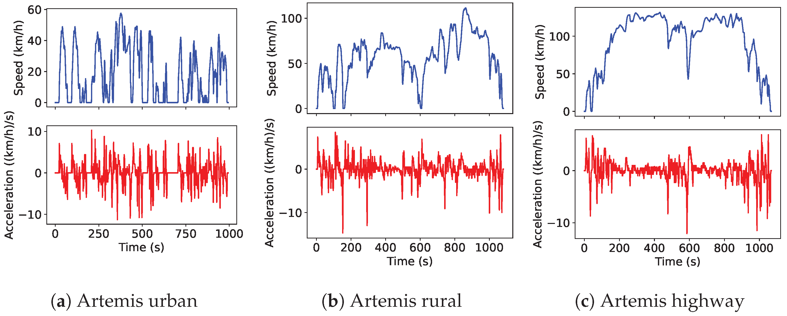
In this study, urban, rural and highway conditions are analysed based on the Artemis driving cycles [20]. The Artemis cycles are commonly employed standard cycles derived through a comprehensive analysis of real-world driving data collected from various regions in Europe and driving conditions. Therefore, these cycles represent a standardised set of driving scenarios that closely mimic the real-world conditions and driving habits experienced by typical drivers. Figure 2 shows the speed and acceleration profiles of the three cycles. The distance driven for Artemis urban, rural and highway cycles is 4.9 km, 17.2 km and 28.7 km, respectively.

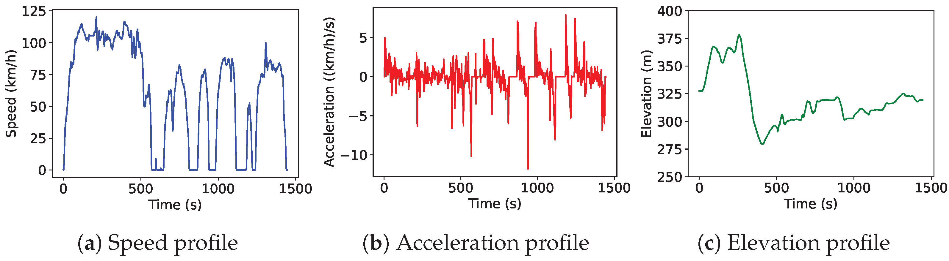
However, the standard cycles do not include road grade profiles, which have a significant impact on the power requirements. The option of including real road grade profiles to the Artemis cycles is discarded, since there is a close relation between speed and inclination (i.e., presumably the maximum speed will not take place when the road grade is the highest). Therefore, in order to include a speed profile with actual road grade information, another cycle is simulated.

The selected cycle, named Real cycle, is derived from the openACC database [21], representing a campaign involving car-following tests on public freeway roads in northern Italy, spanning from Ispra to Cherasco. The data include the speed profile, along with the coordinates, which are utilised to calculate the grade of the road. The profiles of the Real cycle are shown in Figure 3. The Real cycle has a mileage of 25.6 km and represents a mix of rural and highway driving.

A source of uncertainty in driving behaviour is related to the frequency of charging. Some studies suggest that regardless of the arrival State of Charge (SoC) levels, EV users will decide to charge the batteries to the maximum level [22] and it is not necessarily the short-range EV owners who will charge most frequently [23]. In contrast, other studies show that this may not be the case and that charging is affected by the driven distance [24]. This difference in charging behaviour should also be considered when analysing power requirements, as it affects the SoC of the battery.

To reflect this issue, the simulations start on a full battery charge and then two cases are considered: one where the user does the round trip and charges the battery (C1) and another where the user charges the battery every two days (C2), thus completing two departure and two return trips before the charge. The return trips are obtained by reversing the original cycles. Thus, the mileages driven between charges are twice those of the individual cycle for C1 and four times for C2. Another case (C3) is simulated where the starting SoC of the round trip is set to 30%. This case aims to reflect a scenario where the user may have not been able to charge the battery and still needs to perform the driving cycle.

For each of the simulations, the levels of SoH considered are 50–100% with 10% decrements. Therefore, a total of 216 simulations are performed (3 EV models × 4 driving cycles × 3 cases × 6 SoH levels).

2.2. Vehicle Modelling

Vehicle dynamics are modelled considering the forces that act on it (Figure 4).

Aerodynamic drag ($F_a$) is the force that opposes to the relative motion of an object through the air. This force depends on the frontal section of the vehicle ($A_f$), the air density (${\rho }_a$), the aerodynamic drag coefficient ($c_d$) and the velocity at which the car is travelling at a given time ($v_t$). At time t, the aerodynamic drag can be obtained using Equation (1).

$$F_{a,t}=\frac{1}{2}·{\rho }_a·A_f·c_d·v_t^2$$

(1)

The gravitational force ($F_g$) appears whenever the vehicle is circulating in a graded road. It will act as a force opposing to motion if the road grade is positive. The general expression for this force is exposed in Equation (2), where m is the vehicle mass, g is the gravity and $\alpha$ is the road grade.

$$F_g=m·g·sin\left(\alpha \right)$$

(2)

The rolling resistance force ($F_r$) appears when a body rolls on a surface, such as the vehicle tires on the road. It opposes to motion, and it can have big impact on vehicle performance. This force is computed according to Equation (3) where $c_r$ is the rolling resistance.

$$F_r=c_r·m·g·cos\left(\alpha \right)$$

(3)

The traction force ($F_t$) is the force that is needed to overcome resistance and move a vehicle along the road. Based on the Newton’s second law of motion the traction force at time t can be obtained from Equation (4), where $a_t$ represents the acceleration at time t.

$$F_{t,t}-F_{a,t}-F_g-Fr=m·a_t=m·\left(\frac{v_t-v_{t-1}}{\Delta t}\right)$$

(4)

The traction power $P_{t,t}$ (Equation (5)) and the battery power $P_{b,t}$ (Equation (6)) at time t is defined based on the previous computed forces and considering the efficiencies of the electric motor (${\eta }_{em}$) and power electronics (${\eta }_{pe}$). $sgn$ represents the signum function.

$$P_{t,t}=F_{t,t}·v_t$$

(5)

$$P_{b,t}=-P_{t,t}·{({\eta }_{em}·{\eta }_{pe})}^{sgn\left(P_{t,t}\right)}=-F_{t,t}·v_t·{({\eta }_{em}·{\eta }_{pe})}^{sgn\left(P_{t,t}\right)}$$

(6)

The battery power $P_{b,t}$ can also be defined according to Equation (7) based on the battery pack voltage and current, which are affected by battery degradation. In order to simulate the performance at different ageing levels, a battery model that includes the degradation should be employed, as presented in Section 2.3.

$$P_{b,t}=V_{b,t}·I_{b,t}$$

(7)

Combining Equation (7) with Equation (6) and Equations (1)–(4), the necessary battery current to achieve the target speed can be obtained, as shown in Equation (12).

$$I_{b,t}=\frac{(m·a_t+c_r·m·g·cos\left(\alpha \right)+m·g·sin\left(\alpha \right)+\frac{1}{2}·{\rho }_a·A_f·c_d·v_t^2)·v_t}{V_{b,t}}·{({\eta }_{em}·{\eta }_{pe})}^{sgn\left(P_{t,t}\right)}$$

(8)

2.3. Battery Model

As a middle ground between physics-based and data-driven models, the Equivalent Circuit Model (ECM) constitutes one of the most popular alternatives for battery modelling [25]. An ECM consists of electrical components that approximate the various electrochemical and physical processes that occur inside a battery. Different ECMs have been proposed in the literature, including the Rint model or the n-order Thevenin model [26]. A key part of the model selection for this study is related to the availability of parameter data at different SoH levels. As presented later, data from an open source study are employed, which provide parameters for a second-order Thevenin model and thus, this is the selected battery model. It should be highlighted that the use of this type of model is common due to the good trade-off between accuracy and computational cost.

The 2RC ECM, shown in Figure 5, consists of an ideal voltage source ($OCV$) which represents the Open Circuit Voltage (OCV) of the battery for a given state, a series resistance ($R_i$) and two RC pairs ($R_1$$C_1$ and $R_2$$C_2$) consisting on a resistor and a capacitor in parallel.

Considering this 2RC model, the battery voltage at time t ($V_t$) is obtained using Equation (9). To obtain the voltage drop in each of the RC pairs at time t ($U_{j,t}$), the current at time t$I_{j,t}$ is computed using Equation (10) for $j=1,2$.

$$V_t=OC{V}_t-V_{1,t}-V_{2,t}-I_t·R_i$$

(9)

$$I_{j,t}=e^{-\frac{\Delta t}{R_j·C_j}}·I_{j,t-1}+(1-e^{-\frac{\Delta t}{R_j·C_j}})·I_{t-1}$$

(10)

The values of the model parameters ($OCV$, $R_i$, $R_1$, $R_2$, $C_1$ and $C_2$) are taken from an existing study [27]. The work provides the look-up tables of a 2RC model for a 2.1 Ah Lithium-Ion (Li-ion) cell with a NMC + LMO cathode at 25 °C. Two cycling conditions during the first life were considered, one at 25 °C (FL25 °C) and another at 0 °C (FL0 °C) and model parameters were found with median errors below 10%. For specific error ranges of the model, the reader can refer to the original study. For this study, the FL25 °C parameters are considered. The interpolation and extrapolation techniques are used to obtain the model parameters in the working range of SoC [0–100%] and SoH [50–100%]. For each time t, the $So{C}_t$ is calculated and the model parameters are obtained from the look-up tables.

To calculate the SoC, the Coulomb counting technique is employed, as shown in Equation (11) where C is the nominal cell capacity in Ah.

$$So{C}_t=So{C}_{t-1}+\frac{I_t·\Delta t}{C·SoH}$$

(11)

The equations and parameters presented in this section represent a single cell in the EV battery pack. Considering the pack characteristics that are shown in Section 2.1, the cell configuration can be derived and the pack level current $I_{b,t}$ and voltage $V_{b,t}$ at time t can be obtained from Equations (12) and (13), respectively.

$$I_{b,t}=I_t·n_p$$

(12)

$$V_{b,t}=V_t·n_s$$

(13)

Combining the equation of the vehicle dynamics, Equation (12) with Equations (9)–(14) can be used to estimate the cell current for a given speed and state.

$$I_t=\frac{(m·a_t+c_r·m·g·cos\left(\alpha \right)+m·g·sin\left(\alpha \right)+\frac{1}{2}·{\rho }_a·A_f·c_d·v_t^2)·v_t}{(OCV-R_1·I_{1,t}+R_2·I_{2,t}+R_i·I_t)·n_s·n_p}·{({\eta }_{em}·{\eta }_{pe})}^{sgn\left(P_{t,t}\right)}$$

(14)

2.4. BMS Constraints

The BMS plays a crucial role in maintaining the safety of the battery by limiting the operation to a specific working window [28]. In this study, two main constraints are of interest: overvoltage and undervoltage. The allowed the operating voltage of the cell to be set to 3–4.1 V, above or below which the BMS intervenes to guarantee a safe operation.

One notable constraint imposed by the BMS is the mitigation of undervoltage events. In the occurrence of undervoltage, the BMS takes preventive measures by reducing the allowed discharge power. While this is a protective mechanism, it has implications for the overall performance of the simulated driving cycle. The reduction in discharge power directly translates into a decreased speed and acceleration, impacting the driving experience.

As a consequence of the speed decrease, it is necessary to implement a strategy to make sure that the distance covered in the modified profiles is the same as the baseline (i.e., guarantee that the user reaches the destination). To do so, when the speed is limited, it is assumed that the vehicle maintains a constant speed until it covers the distance that would have been travelled with the baseline higher speed. This assumption allows for a simplified representation of the impact of speed reduction on driving times in the simulation, providing a practical approximation.

Another significant constraint imposed by the BMS during driving is related to overvoltage events. To avoid overvoltage and prevent potential damage to the battery, the BMS limits the power [29], which reduces the regenerated energy.

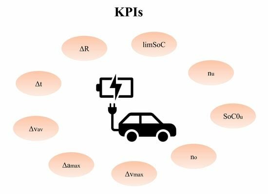
2.5. Key Performance Indicators

The chosen KPIs are selected to serve as effective indicators of significant changes in the driving cycle, as a consequence of the previous BMS restrictions, from a user perspective. The KPIs are provided in

Table 2. Key performance indicators for the study.

Name	Description	Equation
$limSoC$	1 if the capacity is not enough to cover the cycle	-
$n_u$	Number of seconds with undervoltage events	-
$n_o$	Number of seconds with overvoltage events	-
$SoC{0}_u$	Highest SoC at which undervoltage events appear	(15)
$\Delta$$v_{max}$	Max. speed difference during undervoltage events	(16)
$\Delta$$a_{max}$	Max. acceleration difference during undervoltage	(17)
$\Delta$$v_{av}$	Av. speed decrease during undervoltage events	(18)
$\Delta$t	Difference in baseline and modified profile duration	(19)
$\Delta$R	Difference in SoC regenerated during overvoltage events	(20)

, where the baseline profile refers to the original profile of the driving cycle and the modified profile refers to the obtained profiles when the BMS restricts the power during undervoltage or overvoltage events.

$$SoC{0}_u=\underset{i=0}{\overset{n_u}{max}}So{C}_{i,modified}$$

(15)

$$\Delta v_{max}=\underset{i=0}{\overset{n_u}{max}}(v_{i,baseline}-v_{i,modified})$$

(16)

$$\Delta a_{max}=\underset{i=0}{\overset{n_u}{max}}(a_{i,baseline}-a_{i,modified})$$

(17)

$$\Delta v_{av}=\frac{1}{n_u}\sum _{i=0}^{n_u}(v_{i,baseline}-v_{i,modified})$$

(18)

$$\Delta t=t_{modified}-t_{baseline}$$

(19)

$$\Delta R=\frac{1}{A{h}_{cell}}\sum _{i=0}^{n_o}(A{h}_{regen,i,baseline}-A{h}_{regen,i,modified})$$

(20)

$limSoC$ reflects at what SoH the battery runs out of energy to perform the driving cycle. The KPIs $n_u$, $n_o$ and $SoC{0}_u$ are chosen to identify the frequency of underperformance and the highest value of SoC where underperformance occurs. If the driver employs the EV above $SoC{0}_u$, no underperformance should be expected.

The rest of the KPIs are related to the impact of the BMS restrictions on the user experience. The decrease in acceleration ($\Delta$$a_{max}$) is crucial in situations requiring rapid speed increases, such as merging onto a highway or overtaking a vehicle. Maintaining a good speed is important for a good driving experience and to ensure adherence to road norms and overall road safety. The maximum speed decrease is measured by $\Delta$$v_{max}$, but on average, out of $n_u$ undervoltage events, the decrease is reflected by $\Delta$$v_{av}$. The increase in time ($\Delta$t) directly addresses the user’s schedule. The regeneration capability decrease ($\Delta$R) reflects the energy efficiency, impacting environmental considerations and operational costs.

3. Results

Each of the following subsections presents the results for each driving cycle. First the baseline voltage profiles for the three EVs and the C1, C2 and C3 case are shown. Notice that the C1 case corresponds to the first half of the C2 profiles (marked by the dashed vertical line). In each of the plots, the simulation corresponding to 100% SoH and to the lowest simulated value of SoH that can cover the trip, in terms of capacity, is presented. The profiles represent the voltage of the battery without the BMS, that is, allowing the voltage to be outside the operating window. In the timestamps where the voltage falls in the grey area, the BMS acts to bring the voltage to the operating window.

3.1. Artemis Urban Cycle

The voltage profiles corresponding to the Artemis Urban cycle are shown in Figure 6. For all EVs, the voltage often crosses the overvoltage limit in C1 and C2, but stays far from the undervoltage one, even for C3. Notice that the voltage response for 100% SoH appears below that of 50%, as the OCV at a low SoC is significantly lower.

The resulting KPIs for this cycle are presented in

Table 3. KPIs obtained for the Artemis Urban cycle for 100% and 50% SoH.

EV	SoH (%)	Case	limSoC	${\mathit{n}}_{\mathit{o}}$	${\mathit{n}}_{\mathit{u}}$	$\mathit{SoC}{0}_{\mathit{u}}$ (%)	$\mathbf{\Delta }$${\mathit{v}}_{\mathit{max}}$ (km/h)	$\mathbf{\Delta }$${\mathit{a}}_{\mathit{max}}$ ((km/h)/s)	$\mathbf{\Delta }$${\mathit{v}}_{\mathit{av}}$ (km/h)	$\mathbf{\Delta }$t (s)	$\mathbf{\Delta }$R (%)
EV1	100	C1	0	108	0	-	-	-	-	-	0.008
EV1	50	C1	0	313	0	-	-	-	-	-	0.034
EV1	100	C2	0	160	0	-	-	-	-	-	0.012
EV1	50	C2	0	435	0	-	-	-	-	-	0.050
EV2	100	C1	0	22	0	-	-	-	-	-	0.001
EV2	50	C1	0	175	0	-	-	-	-	-	0.011
EV2	100	C2	0	34	0	-	-	-	-	-	0.001
EV2	50	C2	0	269	0	-	-	-	-	-	0.017
EV3	100	C1	0	2	0	-	-	-	-	-	0.000
EV3	50	C1	0	88	0	-	-	-	-	-	0.004
EV3	100	C2	0	4	0	-	-	-	-	-	0.000
EV3	50	C2	0	143	0	-	-	-	-	-	0.006

. For clarity, only the lowest and highest degradation simulated are included (100% and 50% SoH). C3 cases are not included as they do not show overvoltage or undervoltage events. Only KPIs $n_o$ and $\Delta$R are relevant for overvoltage events. As expected, the 50% SoH cases show more overvoltage events and higher decrease in regeneration. However, in all cases, the impact in the regenerated energy is negligible (below 0.05%), especially for the large-capacity EV.

The low impact of the overvoltage coupled with the fact that no undervoltage events were observed, showing the low impact of degradation in urban driving cycles. In addition, considering that most of the regeneration happens under urban conditions [30], it is to be expected that overvoltage events will not create a large issue for other cases. From now on, the cases where overvoltage only is observed are excluded from the analysis for clarity.

3.2. Artemis Rural Cycle

The voltage responses for the Artemis rural cycle are presented in Figure 7. Even if the Artemis rural cycle is more demanding than the urban one, in terms of mileage and speed levels, the results for these simulations also show no undervoltage events for the C1 or C2 cases. However, for the case C3, undervoltage events appear for the short-range vehicle, EV1.

KPIs for those cases with undervoltage are presented in

Table 4. KPIs obtained for the cases where undervoltage occurs for the Artemis rural cycle.

EV	SoH (%)	Case	limSoC	${\mathit{n}}_{\mathit{o}}$	${\mathit{n}}_{\mathit{u}}$	$\mathit{SoC}{0}_{\mathit{u}}$ (%)	$\mathbf{\Delta }$${\mathit{v}}_{\mathit{max}}$ (km/h)	$\mathbf{\Delta }$${\mathit{a}}_{\mathit{max}}$ ((km/h)/s)	$\mathbf{\Delta }$${\mathit{v}}_{\mathit{av}}$ (km/h)	$\mathbf{\Delta }$t (s)	$\mathbf{\Delta }$R (%)
EV1	100	C3	0	3	10	23.3	2.91	2.41	1.28	0.20	0.000
EV1	90	C3	0	3	10	22.6	3.12	2.52	1.55	0.24	0.001
EV1	80	C3	0	4	10	21.6	3.31	2.63	1.83	0.29	0.001
EV1	70	C3	0	7	34	24.4	3.24	2.88	1.09	0.65	0.001
EV1	60	C3	0	8	41	24.0	3.77	3.02	1.07	0.84	0.002
EV1	50	C3	0	8	36	22.9	3.53	2.66	0.73	0.50	0.003

. The KPIs show that, when performing the trip with EV1 at low SoC values, degradation has a slight impact. Undervoltage starts appearing even at 100% SoH, but as the battery ages, the underperformance increases. The maximum speed and acceleration decrease is 3.12 km/h and 2.52 (km/h)/s, respectively, at 90% SoH. However, the number of undervoltage events at this point is still limited (10). This number notably increases at 70% SoH where the BMS reduces the discharge power in 34 points during the trip. Note that the table shows a higher number of undervoltage events for 60% SoH than 50%. This is because, even if the Internal Resistance (IR) is higher at 50%, the ECM at low SoC values shows a higher OCV at 60% compared to 50%, causing the voltage to be lower at certain instances.

The performance of EV1 for the rural C3 case demonstrates the changes that can occur when the speed profile is affected by the BMS restrictions. As an example, the speed profile of the return trip is shown in Figure 8. The effect of degradation is clear when observing the speed profile, especially at 60% SoH.

3.3. Artemis Highway Cycle

Voltage responses for the Artemis highway cycle are presented in Figure 9. Due to capacity fade, EV1 is not able to perform the trip at 80% SoH for C2 and even at 100% SoH for C3. It can be considered that EV1 will never start the journey for C3 and for C2, it will only be able to perform the trip for low values of degradation. EV2 runs out of energy after 70% SoH for C3. Simulations are stopped when the EV runs out of energy to complete the cycle.

Table 5. KPIs obtained for the cases where undervoltage occurs for the Artemis highway cycle.

EV	SoH (%)	Case	limSoC	${\mathit{n}}_{\mathit{o}}$	${\mathit{n}}_{\mathit{u}}$	$\mathit{SoC}{0}_{\mathit{u}}$ (%)	$\mathbf{\Delta }$${\mathit{v}}_{\mathit{max}}$ (km/h)	$\mathbf{\Delta }$${\mathit{a}}_{\mathit{max}}$ ((km/h)/s)	$\mathbf{\Delta }$${\mathit{v}}_{\mathit{av}}$ (km/h)	$\mathbf{\Delta }$t (s)	$\mathbf{\Delta }$R (%)
EV1	100	C1	0	32	4	63.5	0.28	0.25	0.19	0.01	0.007
EV1	90	C1	0	34	8	60.0	1.93	1.84	1.34	0.10	0.009
EV1	80	C1	0	38	9	55.7	3.94	3.70	2.70	0.24	0.011
EV1	70	C1	0	41	27	50.1	4.25	3.75	2.38	0.60	0.013
EV1	60	C1	0	53	115	55.2	4.78	3.78	1.05	1.09	0.016
EV1	50	C1	0	64	196	47.8	5.09	3.87	1.30	2.18	0.021
EV1	100	C2	0	43	66	63.5	7.93	4.03	1.33	1.86	0.010
EV1	90	C2	0	47	372	60.0	12.75	4.97	2.30	18.58	0.013
EV1	80	C2	1	51	271	55.7	24.59	7.24	3.58	19.85	0.015
EV2	50	C2	0	50	3	29.7	0.65	0.65	0.54	0.02	0.010
EV2	100	C3	0	0	6	16.3	3.13	3.13	2.86	0.17	0.000
EV2	90	C3	0	0	6	14.8	3.32	3.32	3.05	0.18	0.000
EV2	80	C3	0	1	6	12.9	3.49	3.49	3.20	0.19	0.000
EV2	70	C3	0	2	13	15.5	5.87	5.29	3.42	0.45	0.000
EV2	60	C3	1	4	10	13.1	6.04	5.26	4.37	0.44	0.000

shows the KPIs for the cases with undervoltage events. Similarly to the previous cycles, for the highway case, no underperformance is observed for the EV3, even at 50% SoH and starting the cycle at 30% SoC.

EV1 shows the highest values of the KPIs for the C1 case. When the battery is new, the EV is able to perform a single go-return cycle with minimum action from the BMS. However, as the battery degrades, the number of undervoltage events increases, taking place even above 50% SoC. At 80% SoH, the speed and acceleration reductions are noticeable, with a maximum value of 3.94 km/h and 3.7 (km/h)/s, respectively. However, only nine undervoltage events are detected. As the SoH decreases, the underperformance becomes more relevant. At 60% SoH, 115 undervoltage events appear with an average speed reduction of 1.05 km/h. At this level of degradation, maximum decreases of 4.78 km/h and 3.28 (km/h)/s are observed for the speed and acceleration, respectively.

For case C2, that has a higher mileage between charges and thus reaches lower SoC values, the EV1 is barely able to perform the driving cycle. At 80% SoH, it does not have enough capacity to cover the trip, but even with a lower degradation (90% SoH), the underperformance is clear. For example, the second return trip for EV1 at 90% SoH is shown in Figure 10. Even if the degradation level is above the commonly assumed EoL threshold, the EV shows a clear underperformance, with a maximum speed reduction of 12.75 km/h and a trip duration increase of 19 s.

Only three undervoltage events are observed for EV2 at 50% SoH, around 30% SoC, and with a minimum impact on the driving for case C2.

For the case C3, EV2 can cover the trip until 60% SoH, but shows important speed reductions before that point. At 70% SoH, the maximum speed reduction is 5.87 km/h and, on average, undervoltage events cause a 3.42 km/h reduction. However, notice that the underperformance starts taking place only at very low values of SoC (below 16%) and there is a low number of undervoltage events.

3.4. Real Cycle

Voltage profiles for the Real cycle are shown in Figure 11. The only case where the EV runs out of capacity to perform the trip is the EV1 at 50% and 90% SoH for C2 and C3, respectively.

Table 6. KPIs obtained for the cases where undervoltage occurs for the Real cycle.

EV	SoH (%)	Case	limSoC	${\mathit{n}}_{\mathit{o}}$	${\mathit{n}}_{\mathit{u}}$	$\mathit{SoC}{0}_{\mathit{u}}$ (%)	$\mathbf{\Delta }$${\mathit{v}}_{\mathit{max}}$ (km/h)	$\mathbf{\Delta }$${\mathit{a}}_{\mathit{max}}$ ((km/h)/s)	$\mathbf{\Delta }$${\mathit{v}}_{\mathit{av}}$ (km/h)	$\mathbf{\Delta }$t (s)	$\mathbf{\Delta }$R (%)
EV1	60	C1	0	73	2	55.6%	1.18	1.19	1.15	0.02	0.015
EV1	50	C1	0	92	2	48.1%	1.48	1.48	1.44	0.02	0.021
EV1	100	C2	0	45	11	53.6%	2.01	1.26	0.95	0.10	0.005
EV1	90	C2	0	52	10	48.8%	2.27	1.80	0.96	0.15	0.008
EV1	80	C2	0	64	12	47.9%	2.36	2.16	0.93	0.17	0.010
EV1	70	C2	0	68	30	51.0%	4.64	3.82	1.57	0.64	0.011
EV1	60	C2	0	83	64	55.6%	6.69	3.46	1.70	1.92	0.016
EV1	50	C2	1	103	90	48.1%	5.90	2.09	1.63	2.43	0.023
EV1	100	C3	0	3	157	24.8	11.83	4.43	2.40	6.16	0.000
EV1	90	C3	0	3	180	24.2	10.31	4.07	2.68	7.98	0.000
EV1	80	C3	1	3	200	27.8	13.37	3.06	2.42	8.29	0.000
EV2	70	C3	0	0	2	15.5	0.79	0.80	0.76	0.01	0.000
EV2	60	C3	0	0	3	13.1	1.13	1.12	1.07	0.03	0.000
EV2	50	C3	0	0	2	9.9	0.83	0.83	0.80	0.01	0.000

shows the KPIs for the cases where undervoltage events occur. Power restrictions have an important impact in the EV performance for the Real cycle. For the user with daily charging (C1), power restrictions start to appear at 60% SoH with a maximum speed reduction of 1.18 km/h. The speed reductions start taking place at mid-SoC values. In fact, the first speed decrease is observed at 55% SoC.

The user with alternate day charging (C2) shows more critical values of the KPIs. The second return trip for this case is presented in Figure 12. As shown, the speed profile is limited in several parts of the trip, with the biggest underperformance being at high speeds at the end of the trip. Underperformance starts even at 100% SoH, although at this stage, it can be considered mild. At low levels of degradation (60% SoH), the underperformance is notable with a maximum reduction of 6.69 km/h in the speed (when the SoC is 15%) and 3.46 (km/h)/s in the acceleration. Notice that, at 50% SoH, the speed reduction seems to be lower, but it is simply because the EV runs out of capacity to perform the last part of the cycle, which is where the most extreme reductions take place. Nevertheless, as reflected by $SoC{0}_u$, speed reductions start around 50% SoC.

For the case C3, both EV1 and EV2 show power restrictions. EV1 cannot correctly perform the cycle even at 100% SoH, with 157 undervoltage events with a 2.4 km/h speed reduction on the average and maximum speed and acceleration reductions of 11.83 km/h and 4.43 (km/h)/s, respectively. EV2 is more suited to perform the cycle. A limited amount of undervoltage events (3–4) start appearing at 70% SoH and below. However, the underperformance is limited (below 1.13 km/h and 1.12 (km/h)/s in all cases) and can be considered negligible.

4. Discussion

The outcomes of this study provided insights into the tangible impact of battery degradation on the overall driving experience of EVs. This is a significant stride towards fostering wider EV adoption, as it empowers consumers with a clearer understanding of how their vehicles will perform throughout their lifespan and manufacturers’ knowledge to aid in battery design.

The 24 kWh vehicle (EV1) is the most likely to notice the degradation during driving. For urban driving, it is not a concern, even at low SoH levels due to the lower power demands for these conditions. For rural driving, the user may notice EV underperformance only when driving below 30% SoC and at moderate levels of degradation. Speed reductions of around 70% SoH start to be frequent. Considering the ageing model presented in [31], the user would start noticing the impact of degradation after 8 years and only sporadically when not being able to charge the battery.

On high-grade roads or for highway conditions, EV1 shows frequent signs of underperformance. For highway only driving, even the less demanding cases (daily charging), show notable speed reductions taking place above 100 km/h at 80% SoH (after 5.5 years [31]), with a maximum value of almost 4 km/h. For users who drive at lower SoC values, the underperformance may be noticeable since the start, showing that low-capacity batteries are not suitable for demanding cycles.

On the other hand, EV2 shows robust performances for urban, rural and rural–highway (Real cycle) conditions even at 50% SoH and low SoC. For this Real cycle, EV2 shows slight underperformances either at 50% SoH driving at high SoC levels or at 70% SoH at low SoC levels. Even if the speed reductions can be high (up to 5.87 km/h), the BMS only restricts the power in a limited number of points. Considering that driving below 30% SoC is not common [32] and that it can take approximately 13 years for a mid-capacity battery to reach 70% SoH [31], it is rare that users of mid-range EVs will notice any level of underperformance.

This is even more clear for EV3, which shows no level of underperformance for any road type, level of degradation or SoC values. It should be highlighted that these results are particular to the cycles simulated; in other real-world scenarios, where speed limits exceed 120 km/h, results may differ.

Therefore, results suggest that higher robustness is expected from mid and long-range EVs compared to short-range ones. Currently these type of EVs are dominating the market (e.g., in 2021 the average capacity of EVs sold in the UK was over 50 kWh [17]). Considering this, high levels of trust could be expected from most EV owners, which can help foster EV acceptance.

The results of this study can help improve the EoL estimation methodologies to guarantee that the EV battery is retired once it is unable to correctly perform. As this study shows, EV batteries encounter various constraints related to capacity and power fade as they age. These constraints can manifest at different points and with different severity depending on factors such as usage patterns and the nominal battery capacity. Consequently, a one-size-fits-all approach to EoL does not seem appropriate or realistic. Thus, there is a need to move beyond the commonly assumed EoL threshold of 70–80% SoH.

By quantifying the impact of these constraints on the driving experience, an improved criterion for a functional EoL can be made. In terms of capacity, the battery should be able to provide the energy required to meet the common driving trips of the user. In terms of power, overvoltage-related limitations have been shown to be negligible and thus, can be excluded from the EoL criteria.

On the other hand, the results have shown how reducing the discharge power affects driving by not being able to reach the required speed or acceleration. If the reduction in performance is large, it can generate dangerous conditions on the road, for example, entering a roundabout without enough acceleration. However, if the undervoltage is small, the implication of the power restriction is low. For example, a 1% reduction in the maximum speed may not be critical or noticeable (e.g., from 120 km/h to 118.8 km/h) and power limitations are also present for conventional vehicles.

Based on the results of this study, a functional criterion for the power-related EoL is made. The proposed approach is to establish a threshold for the maximum allowable speed decrease (i.e., $\Delta$$v_{max}$). By tracking relevant variables during battery operation, it can be estimated if this threshold will be surpassed, thus causing the EoL. The mentioned variables can be either the expected voltage or the power request.

For simulations similar to those presented in this study, it is possible to estimate the expected voltage at each point of the driving cycle, using a battery model, and compare it to the minimum allowed voltage of the battery. This difference is referred to as an undervoltage value. This value is closely linked to the generated speed decrease (i.e., larger values of the undervoltage generate higher speed decreases).

In real applications, however, the information that can be employed is the discharge power requested to the battery at each point. This value can be compared to the maximum available power that is computed by the BMS. Similarly to the undervoltage value, the power difference is also related to the speed decrease (i.e., a larger difference between request and available power generate higher speed decreases).

The speed decrease does not only depend on the undervoltage or power difference; other aspects such as the SoC or SoH affect the level of speed decrease. Nevertheless, it is possible to find a value of the undervoltage that generally creates a speed decrease above an imposed threshold.

To do so, out of all the undervoltage events simulated, the relation between undervoltage and speed decrease is analysed. Among the lowest values, 25% are discarded, meaning that in some cases, low undervoltage values create a larger speed decrease, but are only in extreme situations and do not represent the common relationship. This corresponds to the finding the first quartile (Q1) of the data.

Table 7. EoL criteria considering different speed thresholds.

Speed Decrease Threshold (km/h)	Max. Undervoltage Value (V)	Max. Power Difference (%)
2	0.203	12.46
5	0.319	14.12
10	0.740	31.25

shows, for different speed decrease thresholds, the maximum undervoltage value and power difference that would force the battery EoL.

Estimation of the Functional EoL

In order to illustrate how this information can be practically applied to define a functional EoL for EV batteries, specific examples are presented, involving EV1 and case C1. The same methodology can be applied to all other cases. To do so, the concept of the SoF is introduced [17]. The SoF provides an indicator of how far the battery is from underperforming and thus reaching the EoL. Throughout this paper, the importance of considering both capacity fade and power fade for a comprehensive EoL determination has been emphasised. Following this idea, the SoF is composed of two terms: capacity ($So{F}_c$) and IR ($So{F}_{IR}$).

$So{F}_c$ is calculated using Equation (21) and involves tracking the capacity (C) and comparing it with the required capacity to complete the journey ($C_{EoL}$).

$$So{F}_c=\frac{C-C_{EoL}}{C_{BoL}-C_{EoL}}$$

(21)

In order to estimate the current capacity C, SoH algorithms should be employed. A large number of methodologies have been proposed in the literature to do so, including semi-empirical models [33], ECM-combined with filters [34] or data-driven approaches [35,36]. It is out of the scope to propose a specific algorithm to estimate the SoH, as the goal is to estimate the SoF for predefined SoH levels.

Along with the capacity, during the driving cycle, the IR ($I{R}_t$) is monitored at each timestamp t. In this study, $I{R}_t$ is predefined for each SoH and SoC based on the model parameter tables. In a real BMS application, the IR should be estimated based on available methods [37].

The value of $I{R}_i$ is compared to a maximum value ($I{R}_{t,max}$). $I{R}_{t,max}$ represents the IR that would lead to an undervoltage event at timestamp t. As it has been described, low undervoltage values create a lower underperformance that may not be noticeable to the driver. In this example, a conservative approach is taken by considering a minimum undervoltage of 0.2 V to define the EoL. Thus, $I{R}_{t,max}$ is obtained from Equation (9) by imposing $V_t$ = 2.8 V. To determine $So{F}_{IR}$, the critical point during the driving cycle is identified where $I{R}_t$ is closest to $I{R}_{t,max}$, and these values are referred to as $IR$ and $I{R}_{max}$ in Equation (22).

$$So{F}_{IR}=\frac{I{R}_{max}-IR}{I{R}_{max}-I{R}_{BoL}}$$

(22)

The $SoF$ for a given level of degradation is obtained from Equation (23) which considers the most critical term. Whenever the $SoF$ falls to 0, the battery is considered to have reached EoL.

$$SoF=min(So{F}_c,So{F}_{IR})$$

(23)

Figure 13 shows the relation between SoH and SoF for the four cycles simulated in this study (for EV1 and C1 case). From the figure, the SoH at which the functional EoL is found ($SoF$ = 0) can be observed. In addition, it is possible to observe the cause of the EoL by comparing $So{F}_c$ and $So{F}_{IR}$.

For the Artemis urban cycle, $SoF$ has the same values as $SoH$, indicating that the EoL, in this case, is driven by capacity fade and not power fade (at least until 50% SoH). In fact, the power is not a concern even at 50% SoH, where the $So{F}_{IR}$ is still above 90%. Similar trends are obtained for the Artemis rural cycle, with a faster decrease in $So{F}_{IR}$ in comparison with the urban case.

For the Artemis highway cycle, the EoL is defined by the power constraints, which appear between 100 and 90% SoH. Notice that the exact EoL is between these values and the exact point is not provided as only 10% SoH increments have been simulated. In reality, the estimation of the SoF should be performed frequently (e.g., monthly).

For the Real cycle, the functionality is marked by the capacity fade in the beginning but after 70% SoH power constraints are imposed and end up forcing the EoL at 50% SoH.

These examples demonstrate the importance of understanding the impact of degradation in the ability to meet specific driving trips and how it can be applied to track the functionality of the battery through the SoF, which is employed to define the EoL. The definition proposed for the SoF can be applied in real EVs with the difference that, instead of a single cycle like the examples of this study, the estimation of EoL requirements should be performed by analysing historical trips.

Therefore, for an improved determination of the EoL, a dynamic assessment that considers not just the SoH but also the battery’s ability to meet specific operational requirements is necessary. This approach acknowledges that an EV battery may still have substantial usable life beyond the conventional SoH threshold, provided it can fulfil the demands placed upon it, which strongly vary depending on the user. The implications of this extend beyond individual EVs; a functional EoL definition can be used to optimise battery usage, minimise premature replacements and provide realistic information to businesses interested in the reuse or recycling of the retired battery.

5. Conclusions

This study has performed simulations to understand the impact of degradation on EV performance, with a specific focus on the pivotal role played by the BMS in regulating power to maintain the battery voltage in the allowed operating window. It is well documented in the literature that battery degradation causes a power fade in the battery. However, this study allows for the quantification from a user’s driving experience by focusing on the limitations in speed, acceleration and regeneration capabilities.

Results show the importance of undervoltage events that limit the discharge power and thus, the speed and acceleration that the EV can reach. This study also shows that, in comparison, trip duration and regeneration capabilities are not significantly impacted, even at high levels of power fade. The extent to which users would experience underperformance highly depends on the EV characteristics and the type of driving cycle.

For the short-range EV, the power limitations imposed by the BMS have shown to impact speed and acceleration, manifesting as reductions of up to 6.7 km/h and 3.96 (km/h)/s,, respectively. These values represent extreme reductions once the battery is close to being depleted. For middle SoC values, reductions of around 2–3 km/h are observed. Notably, these constraints are more pronounced under on uphill rural or in highway conditions, particularly at high speeds exceeding 90 km/h and for low SoC values. For other driving cycles, like urban or flat rural, the short-range EV meets the requirements without any underperformance events.

The mid-range EV simulated, similar to those currently dominating the market, has displayed no signs of underperformance for rural and urban conditions, even at extreme degradation levels and low SoC values. For highway conditions, the mid-range EV shows a robust performance unless the cycle is performed starting at low SoC values, which does not represent common driving habits. In addition, by the time the mid-capacity battery reaches low SoH levels, it is likely that the EV itself has had to be replaced beforehand.

The long-range EV has shown a robust performance regardless of the road type and SoH level, even if the cycles are performed starting at 30% SoC. Thus, the results suggest that users with mid- and long-range EVs and with common driving requirements will not notice a decay in the performance during the lifespan of their EV.

The fact that short-range EVs show a limited performance when subjected to demanding cycles (e.g., highway conditions) is a sign of why the 80% SoH limit was established. Nevertheless, currently, there are hardly any vehicles with these battery capacities being sold, which underscores the importance of redefining the EoL criteria to individual cases.

In that sense, the analysis presented in this study can serve as a foundational pillar for optimising EoL estimations, beyond the simplistic criteria of the fixed threshold. This knowledge not only informs the research and industry but also plays a crucial role in fostering user confidence and the acceptance of EVs as a reliable and viable option to meet their transportation needs throughout the lifetime of the vehicle.