
Computational Fluid Dynamics Modeling of Concrete Flows in Drilled Shafts
by
Jesudoss Aservitham Jeyaraj
,
Anthony Perez
,
Abla Zayed
,
Austin Gray Mullins
and
Andres E. Tejada-Martinez
* Department of Civil & Environmental Engineering, University of South Florida, Tampa, FL 33620, USA
*
Author to whom correspondence should be addressed.
Fluids 2024, 9(1), 13; https://doi.org/10.3390/fluids9010013
Submission received: 2 November 2023
/
Revised: 24 December 2023
/
Accepted: 26 December 2023
/
Published: 31 December 2023
(This article belongs to the Special Issue Advances in Computational Mechanics of Non-Newtonian Fluids)
Abstract
:Drilled shafts are cylindrical, cast-in-place concrete deep foundation elements. During construction, anomalies in drilled shafts can occur due to the kinematics of concrete, flowing radially from the center of the shaft to the concrete cover region at the peripheral edge. This radial component of concrete flow develops veins or creases of poorly cemented or high water-cement ratio material, as the concrete flows around the reinforcement cage of rebars and ties, jeopardizing the shaft integrity. This manuscript presents a three-dimensional computational fluid dynamics (CFD) model of the non-Newtonian concrete flow in drilled shaft construction developed using the finite volume method with interface tracking based on the volume of fluid (VOF) method. The non-Newtonian behavior of the concrete is represented via the Carreau constitutive model. The model results are encouraging as the flow obtained from the simulations shows patterns of both horizontal and vertical creases in the concrete cover region, consistent with previously reported field and laboratory experiments. Moreover, the flow exhibits the concrete head differential developed between the inside and the outside of the reinforcement cage, as exhibited in the physical experiments. This head differential induces the radial component of the concrete flow responsible for the creases that develop in the concrete cover region. Results show that the head differential depends on the flowability of the concrete, consistent with field observations. Less viscous concrete tends to reduce the head differential and the formation of creases of poorly cemented material. The model is unique, making use of state-of-the-art numerical techniques and demonstrating the capability of CFD to model industrially relevant concrete flows.
1. Introduction
Drilled shafts are cylindrical, cast-in-place concrete, deep foundation elements used for heavy structures such as highway bridges and tall buildings. These foundations are often the best option from the aspects of cost-effectiveness, applicability to the variety of soil strata encountered, and minimum disturbance in terms of noise and vibrations to surrounding structures.
Construction of drilled shafts involves the excavation of a cylindrical void in the soil using large-diameter augers and subsequent concreting after placing the necessary reinforcement. A highly engineered drilling fluid, called slurry, is used to maintain the stability of the excavation prior to concreting by maintaining the slurry head within the excavation 1.2 to 2 m higher than the surrounding groundwater (Figure 1). Slurry can be a combination of polymer, clay mineral, or a combination of both mixed with water to form a viscous fluid that is slow to penetrate the surrounding soils.
After the excavation is completed to the required depth (filled with slurry) and steel reinforcement has been placed, concreting is performed from the bottom up via a tremie or rigid pump line extending to the bottom of the excavation. As sketched in Figure 1d,e, concrete displaces the drilling fluid and fills the excavation. While the concreting is taking place the tremie pipe can be withdrawn in stages or might be left near the bottom for the entire concrete pour.
The rising concrete interacts with the drill fluid and forms an interface layer called laitance which is characterized by a higher water/cement ratio material caused by the mixing action of the moving concrete and displacing slurry. Best construction practice recommends overpouring the concrete once it reaches the surface to expel all compromised concrete, the laitance. Therefore, as a rule, any concrete/slurry interface regardless of where it occurs results in poor-quality concrete. This is an important distinction which is discussed later.
Even though drilled shaft construction dates to the 1950s, the occurrences of anomalies have not been eliminated which include soil inclusions, trapped slurry pockets, reduction in shaft cross-sectional area, and exposed steel reinforcement. One of the main reasons for anomaly formation is attributed to the kinematics of the concrete flow. Physical studies have shown the rising concrete level in the shaft excavation is affected by the presence of the reinforcing cage where measurements of the rising concrete level inside and outside the cage consistently showed higher concrete levels within the cage (Figure 1d,e, Figure 2a and Figure 3a) [2,3]. The head differential (Hdiff) increases with higher concrete placement velocity and with tighter steel bar spacing which restricts radial flow. Deese and Mullins [3] showed that when a sufficient amount of pressure is achieved by the rising concrete head within the cage, only then is the concrete forced through the reinforcing cage.
Bowen [4] was the first to show vestiges of trapped clay slurry products in the creases that form as the concrete flows through the reinforcement cage. The radial concrete flow is cleaved by the vertical and horizontal rebars (Figure 2b and Figure 3b) and does not fully rejoin on the outside of the cage (Figure 3c). This provides an inherited opportunity for laterally forming laitance interfaces to become trapped, creating creases in the cover concrete (Figure 2b) and projecting the reinforcement cage layout to the outer concrete surface (Figure 2c). This phenomenon has been termed “mattressing” by the Deep Foundations Institute due to the quilted mattress top appearance [5]. The laitance interfaces contain poorly cemented or high slurry-cement ratio material, which increases the rate of sulfate or chloride ingress. Bowen [4] also confirmed the creases extended full depth to the steel and the concrete was not contiguous across the creases.
Figure 2.
Experiments of concrete flows around rebars [2,6,7]: (a) The development of head differential, Hdiff in concrete flow across the rebar cage in a shaft. (b) The development of creases as cement flows around a rebar in a concrete shaft. (c) Creases at the concrete side walls of the shaft form a mattressing pattern.

Figure 3.
Conceptual sketches of concrete flow round rebars in a shaft. (a) Elevation view of concrete flow revealing radial flow component through rebar cage and associated head difference across the cage, Hdiff. (b) Top view of concrete flowing radially past rebar cage showing initial development of creases. (c) Top view of developed creases in the concrete cover region characterizing a poorly cemented shaft.
Short of the few cases where drilled shafts have been exhumed or where large-scale laboratory studies have been conducted, the concrete flow patterns in drilled shafts remain largely unknown which leaves the as-built state of underground structures also unknown. Hence, there is a need to understand the variables that lead to undesirable crease formations that leave reinforcing steel exposed to rapid degradation. This study focused on developing a CFD model that can represent the flow patterns of concrete in drilled shafts. This included specific attention to the head differential across the reinforcing cage and the variables influencing this differential (Hdiff). Integrating such a model with rheological analysis of the concrete mix promises a scientifically robust approach to future drilled shaft concrete casting.
In this study, a CFD model of fresh concrete flow in drilled shaft excavation was developed considering (1) realistic concrete flow rheological properties (based on the Carreau constitutive model) and (2) as-built cages that formed flow pathway blockages. The three-dimensional non-Newtonian CFD model was developed using the finite volume method incorporating the VOF method to track the motion of the interface between the concrete and the drilling slurry. The model was tested with two types of concrete, a viscous concrete leading to a head differential across the reinforcing cage and a significantly less viscous fluid characterized by greater flowability through the cage, resulting in a more uniform (idealized) flow (see sketches in Figure 4). Using the model, the effects of the pouring rate of concrete (i.e., the concrete inflow velocity) and the reinforcing cage spacing on Hdiff were investigated.
Computational modeling of fresh concrete flow can be categorized into three distinct approaches, as outlined by [8]. The first approach views concrete as a collection of individual particles. The second treats concrete flow as a continuous, fluid substance. The third approach combines these perspectives, considering concrete as individual particles suspended within a fluid. Readers seeking in-depth information on these methodologies are encouraged to refer to the comprehensive reviews by Gram and Silfwerbrand [8], Vasilic et al. [9], and Roussel and Gram [10], which offer detailed insights into each approach.
This study adopted the second approach in which the concrete is modeled as a single-phase fluid. This approach has been shown to be suitable for simulating self-consolidating concrete (SCC) [11], which is designed to exhibit favorable flow characteristics even in the presence of tight rebar spacing as is the case in drilled shafts [2]. Self-consolidating concrete, alternatively referred to as self-compacting concrete, is an extremely fluid and non-segregating type of concrete with low yield stress. It has the unique ability to spread by itself and surround reinforcement structures without requiring any mechanical aid (vibration) for consolidation [12].
2. Governing Equations
2.1. Incompressible Navier-Stokes Equations
Fluid motion is governed by the incompressible Navier-Stokes equations
and the incompressibility condition
where is the velocity vector, is the gravitational acceleration vector, is the surface tension vector, is the fluid density, and is the viscosity.
2.2. The Volume of Fluid Method
The Volume of Fluid (VOF) method is used to account for the multi-fluid nature of the flow with the density and viscosity defined in Equations (3) and (4), respectively,
where, and are the densities of concrete and slurry and and are the viscosities of concrete and slurry, respectively, and is the volume fraction of the concrete. The VOF method keeps track of the volume fraction occupied by the two fluids: the fluid corresponding to pure concrete at grid cells with ; the fluid corresponding to slurry at cells with . At cells where , the fluid is a mixture of concrete and slurry with the middle of the interface between the two fluids corresponding to . The volume fraction was tracked via solution of a transport equation for , which corresponds to the conservation of mass equation of the concrete:
where the fluid velocity , obtained from Equation (1), is the velocity of the concrete and slurry at cells where and , respectively, and to the velocity of the concrete-slurry mixture at cells where .
2.3. Surface Tension
There are various approaches for incorporating the effect of surface tension between two fluids (slurry and concrete in this case). A popular approach is based on the continuum surface force (CFS) model of Brackbill et al. [13], consisting of the momentum source term in (1) defined as
where is the surface tension between the two fluids and is the curvature of the interface between the two fluids. The curvature is defined as
where is the interface normal vector obtained from the gradient of the volume fraction, that is, and in (6) is only active along the interface between the two fluids, as is spatially constant away from the interface.
2.4. Constitutive Model
Concrete in its fresh state will be modeled as a non-Newtonian shear thinning fluid in which viscosity decreases under shear strain. For example, in the case of SCC, shear thinning is a crucial aspect of its design. When SCC is not being agitated or is under low shear conditions, it has a higher viscosity. This property helps it maintain its homogeneity, preventing the aggregates from segregating or settling. When SCC undergoes higher shear rates, such as during pouring and placement, its viscosity decreases, allowing it to flow easily. This shear thinning property is essential for SCC to flow and fill complex forms and around congested reinforcements without the need for external vibration.
The well-known Carreau model [14] can be used to describe the shear thinning behavior of concrete. In this model, the viscosity is defined as
a function of the shear rate
where the rate of deformation tensor is
In (8), is the is the viscosity at zero shear rate, is the viscosity at infinite shear rate, is a relaxation time constant, and is the power index. With this model, at low shear rate < the fluid exhibits Newtonian behavior and at high shear rate > the fluid exhibits a non-Newtonian power law behavior.
The Carreau model equation in (8) provides a curve-fit through the viscosities of both Newtonian () and shear-thinning non-Newtonian fluids, thus it was taken to model the viscosities for the concrete (shear-thinning) and the slurry (Newtonian). For concrete, and were set as and s, respectively.
3. Computational Setup
3.1. Model Geometries
The basis for the model is the drilled shaft with the concrete flowing into the shaft from the tremie pipe and the slurry flowing from the excavation displaced by the concrete (Figure 4). Four three-dimensional model geometries were developed in SolidWorks [15], two with 48-inch and two with 36-inch diameter shafts (Figure 5). All model geometries were 20 inches in height or depth and span a 90-degree segment of the real cylindrical geometry for computational efficiency.
The two 48-inch diameter shaft models (denoted as models 1 and 2) are characterized by different reinforcements. Model 1 has 4 vertical rebars at 7-inch spacing and 4 horizontal ties at 6-inch spacing. Model 2 has 8 vertical rebars at 3.5-inch spacing and 6 horizontal ties at 3.5-inch spacing. Similarly, the two 36-inch diameter shaft models (denoted as models 3 and 4) are characterized by different reinforcement cages. Model 3 has 3 vertical rebars at 6.3-inch spacing and 4 horizontal ties at 6-inch spacing. Model 4 has 5 vertical rebars at 3.8-inch spacing and 6 horizontal ties at 3.5-inch spacing. These model characteristics are listed in Table 1. The vertical rebars are 1-inch in diameter and the horizontal ties were 1/2-inch in diameter. In all models, the reinforcement cages were placed with a six-inch cover (i.e., the distance from the cage to the outer edge of the excavation was 6 inches).
Tremie pipes of sizes 12 and 10 inches were considered for the 48-inch and 36-inch diameter shafts, respectively. In all models, the tremie was placed from the top of the shaft to six inches above the shaft bottom.
.
3.2. Boundary Conditions
Figure 6 depicts the boundary conditions for the models. Even though in practice concrete is poured from the top of the tremie pipe, the inlet for the concrete flow was set at the bottom of the tremie pipe (see sketch in Figure 4) to reduce the size of the domain and thus, the number of grid cells. The outlet was set at the top of the excavation. Velocity was prescribed at the inlet and pressure was prescribed at the outlet. The inlet velocity value was calculated from the concrete delivery rate in the field, typically consisting of a 10 cubic yard capacity truck depositing all its concrete in 20 min. Thus, the inlet velocity for the 48-inch and 36-inch shafts were 17.1 ft/min and 25.6 ft/min respectively. The outlet pressure was set equal to the atmospheric pressure. No-slip conditions were set at several boundaries of the model: at the outer edge of the shaft excavation, at the tremie pipe, at the bottom of the excavation and at the rebar cage (i.e., at the vertical and horizontal bars). Symmetry boundary conditions were assigned at the azimuthal ends of the 90-degree segmented domains.
3.3. Computational Grids
Unstructured grids were selected to capture all details of the model geometry (the shaft excavation, tremie pipe, vertical rebars and horizontal ties) without incurring a prohibitive computational cost. Grid sizes ranged between 0.033 and 0.13 inches to faithfully capture the 1-inch diameter of the rebars and 1/2-inch diameter of the ties, and thus resolve the formation of creases as the concrete flowed around these reinforcements. Grid cell sizes and number of cells and nodes for models 1–4 are given in Table 2 and the grids for models 1 and 3 are shown in Figure 7, highlighting the finer resolution around the rebars and ties.
3.4. Material Properties
The Carreau model described earlier was used to calculate the viscosity of the concrete in the Navier-Stokes equations governing the concrete flow. Simulations with each model (models 1–4) were carried out first with rheological properties representative of normal concrete (NC) [16] and then with a less viscous concrete (LVC) more representative of SCC for comparison. In all simulations the drilling fluid was taken as slurry. For both NC and LVC, the viscosity values at zero shear rate () and at infinity shear rate () are given in Table 3. For NC, Pas corresponds to the upper empirical value of plastic viscosity reported by Banfill [16]. Slurry was taken to be Newtonian; thus the viscosity was set to be constant. Constant density values were assigned for NC, LVC, and slurry (Table 3). Further characterization of the rheological properties of the NC is given in the Appendix A, in particular the significance of the zero-shear rate viscosity taken as Pas.
The effects of surface tension were tested in preliminary two-dimensional simulations conducted by Jeyaraj [17]. Studies were carried out for surface tension values N/m with the CFS model described earlier in Section 2.2, and results were found independent of . Furthermore, the Weber number [18], a ratio of inertial forces to surface tension forces in the flow, was computed and found that inertial forces are significantly greater than surface tension forces. Thus, the 3-D model simulations were conducted without surface tension.
3.5. Numerical Methods and Computations
Implementation of the model made use numerical approximations of the governing equations that are standard throughout the computational fluid dynamics community, thus the ANSYS Fluent platform (version 18.2) [19] was used to carry out the simulations. The discretization schemes included gradient reconstruction based on second order least squares, approximation of advective terms via second order upwinding, and time stepping via first order Euler. Pressure interpolation was performed via a body-force-weighted scheme. The concrete-slurry interface was represented via a geometric reconstruction which assumes that the interface has a linear slope within each cell it occupies to approximate advective fluxes across the faces of the cell.
The time step size range of 0.01–0.025 s was chosen to ensure stability of the computations. All cases ran up to 2 min of flow time. Initially, at , the shaft was filled with slurry at rest prior to concrete being released from the inlet at the bottom of the tremie pipe as described earlier. The computations with these time steps, time length, and the grid sizes summarized in Table 2 required parallel computing to be carried out in a reasonable amount of time. Hence, the analysis was performed on parallel computers available through CIRCE (Central Instructional Research Computing Environment) at University of South Florida.
4. Results
The flow of concrete and slurry in the drilled shafts simulated is discerned in terms of the volume fraction of concrete, , obtained on horizontal planes at different depths and on vertical planes of the shafts. Recall fluid corresponding to concrete at grid cells had , slurry , a mixture between concrete and slurry , and corresponded to an equal mix of the two fluids.
Figure 8 shows the distribution of concrete (red) and slurry (blue) obtained from the model 4 simulation with NC at flow time = 35 s. A mattressing pattern of creases develops in the concrete cover region as the NC flows around the rebars and ties. Similar patterns were observed in the field [2,3,7] and lab [4] (see Figure 2c).
The distribution of on vertical planes of the drilled shaft also shows the development of a significant concrete head differential, Hdiff, between the inside and the outside of the rebar cage for the flows with NC (Figure 9b,f).
Comparing Figure 9a,b with Figure 9c,d, corresponding to model 1 with NC and LVC, respectively, the presence of creases is noticeably absent in the case of LVC. Furthermore, the value of Hdiff is greatly reduced with LVC relative to NC.
Table 4 lists the maximum Hdiff values obtained for each model simulated with NC and LVC. In the simulations, Hdiff built up over time eventually decreasing as the amount of slurry in the shaft continually decreased over time. For all models simulated, employing the LVC lead to a more uniform upward flow of concrete and thus a value of Hdiff much less than with NC. For example, in model 4, NC leads to a maximum head difference of 12.50 in whereas the LVC lead to a maximum head difference of 1.25 in.
From Table 4, several trends in Hdiff can be observed for the drilled shafts with NC. For models with shaft diameters of 48-inch (models 1 and 2), the smaller cage spacing in model 2 of approximately 5 in. (compared to 9 in. in model 1) lead to a greater maximum Hdiff of 10.75 in. (compared to 4 in. in model 1). A similar trend in maximum Hdiff is also observed comparing the models with shaft diameters of 36 in. (models 3 and 4) with NC in Table 4. Overall, this trend shows that the head differential increases with decreasing reinforcement cage spacing, as the latter causes greater obstruction to the flow of concrete. Furthermore, these results are consistent with the creases observed in the concrete cover regions of models 1 and 2 with NC forming due to the radial outflow of concrete across the reinforcement cage induced by the head differentials (Figure 9a,e).
Table 4 gives insight into the dependence of maximum Hdiff on the upward flow velocity in the shafts for fixed cage spacing. Note that by conservation of mass and from the velocities in the tremie pipes serving as the inlet velocities, the nominal upward velocities in the 48-inch diameter shafts (models 1 and 2) and in the 36-inch diameter shafts (models 3 and 4) are calculated as 1.15 ft/min and 2.07 ft/min, respectively. These nominal velocities correspond to the outlet velocities listed in Table 4. Comparing models 1 and 3 with NC in Table 4, it can be concluded that for a fixed cage spacing of 9 in., a greater nominal velocity in the shaft gives rise to a greater value of maximum Hdiff. A similar conclusion can be made comparing models 2 and 4 with NC in Table 4, both having a cage spacing of 5 in. The dependence of Hdiff on upward flow velocity with the LVC is not as pronounced as with NC.
This previous trend with NC is consistent with the field measurements of shafts with varied cage spacing and concrete flow rates [2,3] plotted in Figure 10. This figure shows the variation of maximum head differential for various values of the cage spacing-to-maximum aggregate diameter (CSD) ratio, where CSD ranged from 6 to 26. Results from the simulations with models 1–4 with NC for a fixed cage spacing (5 in. and 9 in.) are also plotted in Figure 10, showing agreement with field data where wider cage spacing demonstrated smaller Hdiff values. This agreement is attributed to the fact that the concrete in the models was taken to be homogenous, thus no aggregates were present.
5. Summary and Conclusions
A 3-D CFD model was developed to simulate the concrete flow in a tremie-placed drilled shaft excavation. The model was developed considering the rheological properties of both concrete and drilling fluid (slurry) leading to qualitative prediction of the flow pattern around rebars and ties. The non-Newtonian Carreau model was used to describe the rheological behavior of the concrete while the drilling fluid was taken as a Newtonian fluid. The VOF method was used to track the interface between the concrete and the slurry.
A qualitative validation of the 3-D model simulations with NC was presented based on comparisons with field-collected data. The patterns of vertical and horizontal creases in the concrete cover region obtained from the simulations were consistent with the patterns of creases developed in field and laboratory cast shafts in previous works [2,3,7]. In addition, the concrete head differentials observed in the flow pattern from the simulation were comparable to the field values.
Further, via the model simulations, it was observed that the use of a lower-viscosity fluid compared to normal concrete produced negligible creases in the concrete cover region and the concrete head differentials were minimal. In the case of NC, there were creases of considerable depth in the shaft concrete cover region and the concrete head differential was 4 to 12 inches depending on the shaft size and the reinforcement cage arrangement.
From the above comparison made between the concrete flow patterns obtained from the simulation and the experimental physical studies, it can be concluded that the 3-D model developed provides qualitative yet representative results. It is not possible to make a stronger comparison between the model and physical experiments because the flow time was not measured in the field. Furthermore, the concrete was modeled as a homogeneous fluid, thus it did not consider the coarse aggregates present in the concrete.
The development of the present numerical model and subsequent evaluation of the concrete flow performance are unique while making use of state-of-the-art numerical techniques and physical modeling. As a next step, this model should be extended to particles in fluid-suspension to simulate a more realistic concrete flow pattern with suspended aggregates. Also, the same approach of modeling and simulation, can be applied to other concrete flow scenarios such as flow in a barrette (a rectangular shaped deep foundation element) and in diaphragm walls (an underground earth retaining structure with rectangular panel walls) which are extensively used in the transportation industry. Therefore, this modeling approach has the potential for further research in various applications of underground structures where flow patterns are unknown. Finally, as is discussed in greater detail in the Appendix A, integrating such a model with numerical and laboratory rheological analysis of the concrete mix promises a scientifically robust approach to underground concrete casting. This approach could potentially be adopted by practicing engineers as CFD and high-performance computing resources become democratized and thus accessible to non-CFD experts (e.g., see Engler Faleiros [20]).
Author Contributions
Conceptualization, A.Z. and A.G.M.; Methodology, A.P. and A.E.T.-M.; Software, J.A.J., A.P. and A.E.T.-M.; Validation, J.A.J. and A.P.; Formal analysis, J.A.J. and A.E.T.-M.; Data curation, J.A.J.; Writing—original draft, J.A.J.; Writing—review & editing, A.Z., A.G.M. and A.E.T.-M.; Supervision, A.E.T.-M.; Funding acquisition, A.Z. and A.G.M. All authors have read and agreed to the published version of the manuscript.
Funding
This research no external funding.
Data Availability Statement
Data are available upon request.
Conflicts of Interest
The authors declare no conflicts of interest.
Appendix A. Concrete Rheology
Concrete, traditionally considered as a Bingham plastic in its non-Newtonian fluid form, requires a shear stress () greater than a threshold or yield stress () to deform, otherwise remaining rigid for . Figure A1a shows a sketch of the flow curve for a Bingham plastic, characterized by a linear relationship between and the shear rate () for with slope given by the plastic viscosity . This linear relationship implies that a Bingham plastic does not exhibit shear thinning nor thickening, as the concrete maintains its structure when exceeds . However, when concrete such as SCC is subjected to shear surpassing , for example during the processes of pouring and placing, its viscosity diminishes (indicative of shear thinning, Figure A1a), facilitating smoother flow.
It is important to stress that the rheology of concrete is complex beyond that of a Bingham plastic or shear thinning fluid, exhibiting thixotropy and in some instances shear thickening in the case of SCC ([16]; Figure A1a). Thixotropy refers to the concrete becoming less viscous when shearing is applied and recovering its more viscous state over time after the shearing is stopped. This behavior implies a time dependency of the viscosity, which is neglected when the concrete is modeled as a Bingham plastic or as a pseudoplastic (shear thinning). Furthermore, given its low yield stress, researchers have used thickeners in SCC to prevent the segregation between its coarser particles and its fine contents (such as fine aggregates (sand), binders (cement paste), additives (fly ash, ground granulated blast furnace slag, silica fumes), and water [16].
Figure A1.
(a) Sketch of flow curves for a Newtonian fluid, shear thinning, shear thickening, and Bingham plastics. (b) Sketch of flow curves for HBB and Carreau models.
Figure A1.
(a) Sketch of flow curves for a Newtonian fluid, shear thinning, shear thickening, and Bingham plastics. (b) Sketch of flow curves for HBB and Carreau models.

Despite the complex rheology of SCC and concrete in general, prior CFD simulations have successfully modeled SCC as a Bingham plastic. For example, Vasilic et al. [11] used this approach to simulate the SCC flow in an LCPC box (named after the Laboratoire Central des Ponts et Chaussées (LCPC) in France where it was developed). The LCPC test case consists of a rectangular box in which fresh concrete is held in place by a gate (as sketched in Figure A2a) and suddenly released, spreading over a length (as sketched in Figure A2b).
Although the standard form of the Navier-Stokes equations does not inherently capture the yield stress characteristic of Bingham plastics, the yield stress behavior can be incorporated via the Herschel-Bulkley model for Bingham plastics (henceforth the HBB model). As sketched in Figure A1b, the HBB model approximates a Bingham plastic via two viscosities, the plastic viscosity and a second viscosity defined as , where , is an input parameter. In this fashion, the HBB model approximates the Bingham plastic as a highly viscous fluid with viscosity when .
The Navier-Stokes equations require the divergence of , which is undefined for the model due to the jump in viscosity from to (Figure A1b). This difficulty can be circumvented via a regularization of the viscosity, which in the Fluent solver is expressed as
Following the first expression in (A1), the critical shear rate, , can be related to the viscosity at zero shear rate, , as
Figure A2.
Sketch of LCPC box test case. At , the gate in (a) is removed and in (b) the final state corresponds to when the flow of concrete stops characterized by a final height profile and final spread length .
Figure A2.
Sketch of LCPC box test case. At , the gate in (a) is removed and in (b) the final state corresponds to when the flow of concrete stops characterized by a final height profile and final spread length .
Vasilic et al. [11] performed a Fluent simulation of the spread of SCC in an LCPC box using the HBB viscosity in (A1). Recalling (A2), the critical shear rate parameter was chosen as small as possible (leading to as high as possible ) without causing numerical instability. For the LCPC box test, the high value of enabled an approximate flow stoppage and thus a nearly time-independent final spread length (Figure A1b), characteristic of physical experiments.
In the present study, the flow of NC and LVC in drilled shafts was simulated using the Carreau model equation in (8) with , exhibiting shear-thinning behavior. Through parameters and , the Carreau model’s continuous viscosity in (8) can be adapted to mimic the regularized viscosity and ultimately the flow curve of the HBB model (as suggested via the sketch in Figure A1). Furthermore, the value of can be chosen sufficiently high to lead to flow stoppage, analogous to the LCPC box test case simulated with the HBB model in [11]. However, the focus of the present study was to demonstrate that a CFD model can exhibit the head differential, Hdiff, observed in drilled shafts, thus was set arbitrarily high ( Pas for NC; see Table 3) without considering flow stoppage.
To assess the performance of the Carreau model used in the present study relative to that of the HBB model, the LCPC box test case was simulated with both models. For simplicity, the flow was solved in two dimensions with the domain and initial condition specified in Figure A2. The box was discretized with 27,000 elements following [11]. The bottom of the box was set as a no-slip wall and the left and right end walls were set as free-slip walls. The top of the box was set as a pressure outlet. The VOF method was used to track the interface between the concrete and the air. The Carreau model (in Equation (8)) was set with the NC rheological parameters specified for the drilled shaft simulations presented earlier ( Pas, Pas, ). Accordingly, the HBB model was set with Pas and following Equation (A1) with Pas. The yield stress in (A1) was set as Pa with plastic viscosity Pas, based on the empirical range of values of and for normal concrete reported by Banfill [16].
The shear stress and viscosity versus shear rate predicted by the Carreau and HBB models with the parameters previously discussed are shown in Figure A3. The height profiles of the concrete in the LCPC box flow predicted by both models at different times are shown in Figure A4. As can be seen, the predicted profiles by the two models are nearly indistinguishable. This may be attributed to the fact that the shear stress predicted by the models is very close for low shear rates (Figure A3a).
In the case of the drilled shafts simulated earlier, it is expected that both models would lead to similar results given the small shear rates occurring in these flows. For example, considering a nominal upward velocity of 1.15 ft/min. in the modeled 48-inch diameter shafts (see Table 4) with a 6-inch concrete cover leads to an approximate nominal shear rate upper bound of 0.038 s−1, for which the Carreau and HBB models predict nearly identical shear stresses (Figure A3a). A similar conclusion can be reached for the modeled 36-inch diameter shafts (Table 4).
Figure A3.
(a) Shear stress and (b) viscosity versus shear rate predicted by the Carreau and HBB models in the simulations of the LCPC box test case.
Figure A3.
(a) Shear stress and (b) viscosity versus shear rate predicted by the Carreau and HBB models in the simulations of the LCPC box test case.

Figure A4.
Concrete height profiles at various times predicted by the Carreau and HBB models in the LCPC box flow test case.
Figure A4.
Concrete height profiles at various times predicted by the Carreau and HBB models in the LCPC box flow test case.

The above analysis suggests that the performance of the Carreau model can closely follow that of the HBB model (used by other researchers) for the concrete flows studied. In the future, prior to performing physical experiments of concrete flow in drilled shafts to further validate the CFD simulations with either the Carreau or the HBB model, the rheological properties of the concrete required by these models should be measured via the LCPC box test case. In particular, the viscosity necessary for these models to capture flow stoppage should be carefully obtained via simulations and physical experiments of the LCPC box flow, as was done in [11]. This should lead to greater accuracy of the modeled concrete flow in drilled shafts through the complete concrete pouring process and subsequent casting to better capture and understand the formation of creases in the concrete cover region.
References
- Brown, D.; Turner, J.; Castelli, R. Drilled Shafts: Construction Procedures and LRFD Design Methods; FHWA NHI-10-016, NHI COURSE NO. 132014 GEOTECHNICAL ENGINEERING CIRCULAR NO. 10; U.S. Department of Transportation Federal Highway Administration: Washington, DC, USA, 2010.
- Mullins, A.G.; Ashmawy, K.A. Factors Affecting Anomaly Formation in Drilled Shafts-Final Report; FDOT Report; University of South Florida: Tampa, FL, USA, 2005. [Google Scholar]
- Deese, G.; Mullins, G. Factors Affecting Concrete Flow in Drilled Shaft Construction. In Proceedings of the ADSC GEO3, GEO Construction Quality Assurance/Quality Control Conference, Dallas/Fort Worth, TX, USA, 6–9 November 2005; Bruce, D.A., Cadden, A.W., Eds.; 2005; pp. 144–155. [Google Scholar]
- Bowen, J. The Effects of Drilling Slurry on Reinforcement in Drilled Shaft Construction. Master’s Thesis, University of South Florida, Tampa, FL, USA, 2013. [Google Scholar]
- Beckhaus, K. (Ed.) EFFC/DFI Best Practice Guide to Tremie Concrete for Deep Foundations, 1st ed.; Deep Foundations Institute: Hawthorne, NJ, USA, 2016. [Google Scholar]
- Mullins, A.G. Development of Self Consolidating Mix Designs for Drilled Shafts; FDOT Report; University of South Florida: Tampa, FL, USA, 2005. [Google Scholar]
- Mullins, A.G.; Zayed, A.; Mobley, S.; Costello, K.; Jeyaraj, J.A.; Mee, T. Evaluation of Self Consolidating Concrete and Class IV Concrete Flow in Frilled Shafts; FDOT Report BDV 25-977-25; University of South Florida: Tampa, FL, USA, 2019. [Google Scholar]
- Gram, A.; Silfwerbrand, J. Numerical simulation of fresh SCC flow: Applications. Mater Struct. 2011, 44, 805–813. [Google Scholar] [CrossRef]
- Vasilic, K.; Gram, A.; Wallevik, J.E. Numerical Simulation of Fresh Concrete Flow: Insight and Challenges. RILEM Tech. Lett. 2019, 4, 57–66. [Google Scholar] [CrossRef]
- Roussel, N.; Gram, A. (Eds.) Simulation of Fresh Concrete Flow: State of the Art Report of the RILEM Technical Committee 222-SCF; Springer: Dordrecht, The Netherlands, 2014. [Google Scholar]
- Vasilic, K.; Schmidt, W.; Kühne, H.C.; Haamkens, F.; Mechtcherine, V.; Roussel, N. Flow of fresh concrete through reinforced elements: Experimental validation of the porous analogy numerical method. Cem. Concr. Res. 2016, 88, 1–6. [Google Scholar] [CrossRef]
- ACI 237R-07, Emerging Technology Series, “Self-Consolidating Concrete”. Available online: https://rosap.ntl.bts.gov/view/dot/25610/dot_25610_DS1.pdf (accessed on 27 December 2023).
- Brackbill, J.U.; Kothe, D.B.; Zemach, C. A Continuum Method for Modeling Surface Tension. J. Comput. Phys. 1992, 100, 335–354. [Google Scholar] [CrossRef]
- Carreau, P.J. Rheological Equations from Molecular Network Theories. Trans. Soc. Rheol. 1972, 16, 99–127. [Google Scholar] [CrossRef]
- Planchard, D.C.; CSWP. SolidWorks 2015 Tutorial with Video Instruction; SDC Publications: Mission, KS, USA, 2014. [Google Scholar]
- Banfill, P.F.G. Rheology of Fresh Cement and Concrete. In Rheology Reviews; British Society of Rheology: England, UK, 2006; pp. 61–130. [Google Scholar]
- West, R.; Ryde, D.; Astle, M.; Bayer, W. CRC Chemistry and Physics Handbook, 70th ed.; CRC Press, Inc.: Boca Raton, FL, USA, 1989. [Google Scholar]
- Ansys Inc. “ANSYS Release Notes 18.2” August 2017, Ansys, Inc. Southpointe, 2600 ANSYS Drive, Canonburg, PA 15317. Available online: https://www.luis.uni-hannover.de/fileadmin/software-lizenzen/Ueberlassung/ANSYS18.2_ReleaseNotes.pdf (accessed on 27 December 2023).
- Jeyaraj, J.A. Numerical Modeling of Concrete Flow in Drilled Shaft. Doctoral Dissertation, University of South Florida, Tampa, FL, USA, 2018; 124p. [Google Scholar]
- Engler Faleiros, D.; van den Bos, W.; Botto, L.; Scarano, F. TU Delft COVID-app: A Tool to Democratize CFD Simulations for SARS-CoV-2 Infection Risk Analysi. Sci. Total Environ. 2022, 826, 154143. [Google Scholar] [CrossRef] [PubMed]
Figure 1.
Schematic of drilling process with slurry stabilization: (a) Set surface casing; (b) Fill and maintain slurry head; (c) Place steel reinforcement; (d) Pour concrete through tremie pipe; (e) Progressive tremie extraction during concrete placement (adapted from FHWA NHI10-16 [1]).
Figure 1.
Schematic of drilling process with slurry stabilization: (a) Set surface casing; (b) Fill and maintain slurry head; (c) Place steel reinforcement; (d) Pour concrete through tremie pipe; (e) Progressive tremie extraction during concrete placement (adapted from FHWA NHI10-16 [1]).

Figure 4.
Schematic of idealized concrete flow (left) and actual concrete flows (right) displacing the drilling slurry [3]. The concrete (with specific weight γconcrete) is sketched in gray and the slurry in green. The real concrete flow on the right develops a head differential, Hdiff, not observed in the idealized flow on the left.

Figure 5.
(a) Model 1: 48-inch diameter shaft model with 4 vertical rebars and 4 horizontal ties. (b) Model 2: 48-inch diameter shaft with 8 vertical rebars and 6 horizontal ties. (c) Model 3: 36-inch diameter shaft with 3 vertical rebars and 4 horizontal ties. (d) Model 4: 36-inch diameter shaft with 5 vertical rebars and 6 horizontal ties. All models are 20 inches in height or depth.

Figure 6.
Boundary conditions applied. The no-slip condition is enforced at the rebars.

Figure 7.
Computational grids for (a) 48-inch diameter shaft (model 1) and (b) 36-inch diameter shaft model (model 3).
Figure 7.
Computational grids for (a) 48-inch diameter shaft (model 1) and (b) 36-inch diameter shaft model (model 3).
Figure 8.
(a) Cut planes showing NC (red) and slurry (blue) distribution as well as interface mixed zones in terms of volume fraction (). (b) Elevation view of the concrete cover region. (c) Elevation view close to the excavation edge.
Figure 8.
(a) Cut planes showing NC (red) and slurry (blue) distribution as well as interface mixed zones in terms of volume fraction (). (b) Elevation view of the concrete cover region. (c) Elevation view close to the excavation edge.
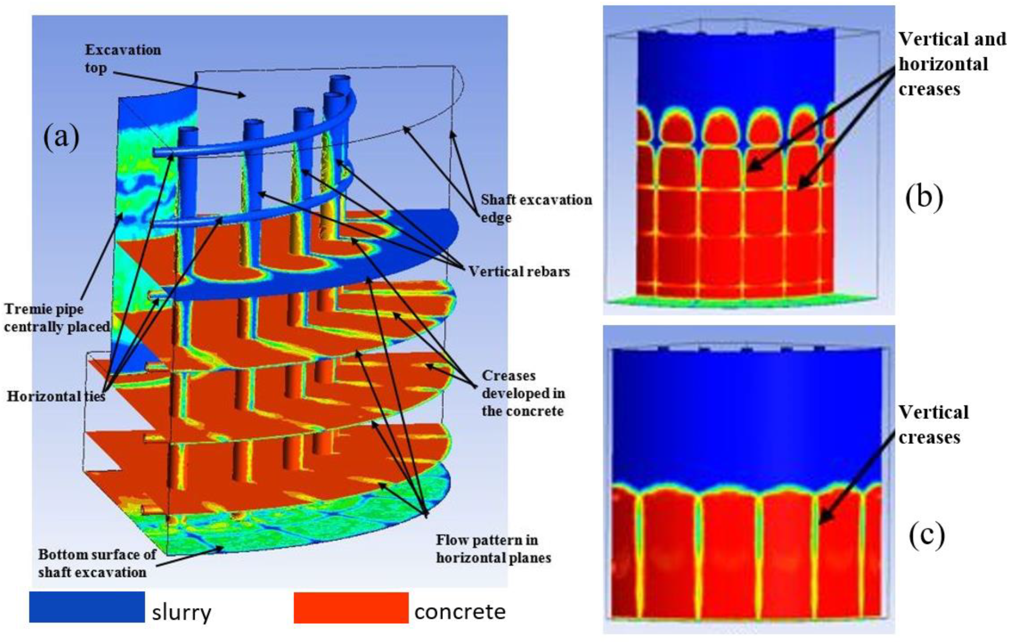
Figure 9.
Volume fraction () on horizontal planes (a,c,e) and concrete cover region (b,d,f)) in models 1 and 2 (see Table 1). (a,b): Model 1 with NC at time = 83 secs. (c,d): Model 1 with LVC at time = 100 secs. (e,f): Model 2 with NC at = 70 secs. = 1 (red) denotes concrete and = 0 (blue) denotes slurry.

Figure 10.
Maximum concrete head differential vs. upward concrete flow velocity in drilled shafts with NC: Comparison between field (physical) data [2] and model simulations [19]. Attention should be directed primarily at the data points, rather than the trends.


Table 1.
Shaft and tremie sizes and reinforcement cage details for each model simulated. Cage spacing (in the last column of the table) is defined as .
Table 1.
Shaft and tremie sizes and reinforcement cage details for each model simulated. Cage spacing (in the last column of the table) is defined as .
| Model | Shaft Size (Diameter) (in) | Tremie Size (Diameter) (in) | Vertical Rebars, Number and Spacing | Horizontal Ties, Number and Spacing | Cage Spacing (in) |
|---|---|---|---|---|---|
| 1 | 48 | 12 | 4 rebars at 7-inch spacing | 4 ties at 6-inch spacing | 9.2 |
| 2 | 48 | 12 | 8 rebars at 3.5-inch spacing | 6 ties at 3.5-inch spacing | 4.95 |
| 3 | 36 | 10 | 3 rebars at 6.3-inch spacing | 4 ties at 6-inch spacing | 8.7 |
| 4 | 36 | 10 | 5 rebars at 3.8-inch spacing | 6 ties at 3.5-inch spacing | 5.2 |
Table 2.
Details of computational grids.
| Model | Mesh Size | Number of Grid Cells | Number of Grid Nodes | |
|---|---|---|---|---|
| Min. (in) | Max. (in) | |||
| 1 | 0.033 | 0.12 | 1,188,233 | 6,366,030 |
| 2 | 0.035 | 0.13 | 1,176,169 | 6,317,274 |
| 3 | 0.03 | 0.11 | 994,014 | 5,326,261 |
| 4 | 0.03 | 0.11 | 1,069,758 | 5,718,755 |
Table 3.
Properties of NC, LVC, and slurry used in the computations.
| Fluid | Density (kg/m3) | s) | |
|---|---|---|---|
| LVC | 2300 | 250 | 25 |
| NC | 2400 | 2500 | 100 |
| Slurry | 1150 | 0.5 | |
Table 4.
Maximum head differential (Hdiff) obtained for each model simulated with NC and LVC.
| Model | Inlet vel. (ft/s) | Outlet vel. (ft/s) | Cage Spacing (in) | Hdiff (in) with NC | Hdiff (in) with LVC |
|---|---|---|---|---|---|
| 1 | 17.7 | 1.15 | 9 | 4.0 | 0.75 |
| 2 | 17.7 | 1.15 | 5 | 10.75 | 1.0 |
| 3 | 25.6 | 2.07 | 9 | 4.50 | 0.75 |
| 4 | 25.6 | 2.07 | 5 | 12.50 | 1.25 |
Disclaimer/Publisher’s Note: The statements, opinions and data contained in all publications are solely those of the individual author(s) and contributor(s) and not of MDPI and/or the editor(s). MDPI and/or the editor(s) disclaim responsibility for any injury to people or property resulting from any ideas, methods, instructions or products referred to in the content. |
© 2023 by the authors. Licensee MDPI, Basel, Switzerland. This article is an open access article distributed under the terms and conditions of the Creative Commons Attribution (CC BY) license (https://creativecommons.org/licenses/by/4.0/).
Share and Cite
MDPI and ACS Style
Jeyaraj, J.A.; Perez, A.; Zayed, A.; Mullins, A.G.; Tejada-Martinez, A.E. Computational Fluid Dynamics Modeling of Concrete Flows in Drilled Shafts. Fluids 2024, 9, 13. https://doi.org/10.3390/fluids9010013
AMA Style
Jeyaraj JA, Perez A, Zayed A, Mullins AG, Tejada-Martinez AE. Computational Fluid Dynamics Modeling of Concrete Flows in Drilled Shafts. Fluids. 2024; 9(1):13. https://doi.org/10.3390/fluids9010013
Chicago/Turabian StyleJeyaraj, Jesudoss Aservitham, Anthony Perez, Abla Zayed, Austin Gray Mullins, and Andres E. Tejada-Martinez. 2024. "Computational Fluid Dynamics Modeling of Concrete Flows in Drilled Shafts" Fluids 9, no. 1: 13. https://doi.org/10.3390/fluids9010013