Article

Trapped Solitary Waves in a Periodic External Force: A Numerical Investigation Using the Whitham Equation and the Sponge Layer Method

by
Marcelo V. Flamarion
1,*,†,
Roberto Ribeiro-Jr
2,†,
Diogo L. S. S. Vianna
2,† and
Alex M. Sato
2,†
1
Unidade Acadêmica do Cabo de Santo Agostinho, UFRPE/Rural Federal University of Pernambuco, BR 101 Sul, Cabo de Santo Agostinho 54503-900, Brazil
2
Departament of Mathematics, UFPR/Federal University of Paraná, Centro Politécnico, Jardim das Américas, Curitiba 81531-980, Brazil
*
Author to whom correspondence should be addressed.
These authors contributed equally to this work.
Fluids 2023, 8(8), 223; https://doi.org/10.3390/fluids8080223
Submission received: 5 April 2023 / Revised: 4 May 2023 / Accepted: 6 June 2023 / Published: 1 August 2023
(This article belongs to the Section Mathematical and Computational Fluid Mechanics)

Abstract

:
This paper concerns the interaction between solitary waves on the surface of an ideal fluid and a localized external force, which models a moving disturbance on the free surface or an obstacle moving at the bottom of a channel. Previous works have investigated this interaction under the assumption that the external force moves with variable speed and constant acceleration. However, in this paper we adopt a different approach and consider the scenario in which the external force moves with variable speed and non-constant acceleration. Using the Whitham equation framework, we investigate numerically trapped waves excited by a periodic external force. Our experiments reveal regimes in which solitary waves are spontaneously generated and trapped for large times at the external force. In addition, we compare the results predicted by the Whitham equation with those of the Korteweg–de Vries equation.

1. Introduction

Humanity has always sought to provide explanations for natural phenomena that occur in everyday life, whether through religious or scientific means. Mathematical models have emerged as an attempt to justify and describe the fundamental laws of nature. While Isaac Newton (1687) was a pioneer in the mathematical theory of water waves, his results lacked mathematical rigor. It was only later that the mathematical formalization of hydrodynamic equations was achieved by Leonhard Euler (1757), who deduced the equations that model the dynamics of water waves which now bear his name [1].
Significant advancements were made in the field of water waves during the 19th and 20th centuries. Mathematical models initially developed for the dynamics of surface water waves are now widely applied in diverse contexts. The Korteweg–de Vries equation (KdV) is a good example of this. Originally formulated in 1895 to describe the dynamics of solitary water waves, it gained notoriety in 1965 with the work of Zabusky and Kruskal [2], who observed that these waves have a particle-like behavior. Solitary waves are now applied in a vast range of areas, such as fiber optics, superconductivity in electronics, particle physics, quantum physics, biology, and cosmology [3,4].
Considerable efforts have been devoted to understanding the interaction between solitary waves and external forces. Such forces can represent a range of physical phenomena, such as atmospheric flows encountering topographic obstacles or flows of water over rocks [5]. Additionally, they can take the form of pressure distributions moving over free surfaces, as seen in ship waves and ocean waves generated by storms when a low-pressure region moves on the surface of the ocean [6].
Due to the numerical and analytical challenges presented by the full nonlinear Euler equations, the study of solitary wave interactions with external forces has mainly been conducted using reduced models, for instance in the KdV framework [7,8,9,10,11,12,13,14,15,16], the fifth-order KdV framework [17,18], and other extensions of the KdV equation [19,20,21,22]. One of the advantages of dealing with these models is that they are completely integrable, which allows for the computation of solitary wave solutions in closed form.
In the weakly nonlinear weakly dispersive regime, the KdV equation is an asymptotic approximation of the full Euler equations. Although this model predicts many interesting nonlinear phenomena such as solitary wave solutions and dispersive shocks, it fails to predict sharp crests, peaking, and wave breaking. With these issues in mind, Whitham [23,24] proposed an ad hoc nonlocal model that has the same quadratic nonlinerarity as the KdV equation; although its linear dispersion relation represents the unidirectional dispersion relation of the Euler equations. This model bears his name, and one of its forms is the Whitham equation:
u t + K u x 3 2 u u x = 0 ,
where u ( x , t ) represents the free surface displacement at position x and time t, ∗ is the convolution operation, and K is the nonlocal operator, for which the Fourier multiplier is defined by
K ^ ( k ) = tanh k k ,
where k denotes the Fourier frequency.
In other terms, the derivation of the Whitham Equation (1) can be roughly explained by the following arguments. We begin by defining the characteristic scales for length, velocity, time, and pressure as h, ( g h ) 1 / 2 , ( h / g ) 1 / 2 , and ρ g h , respectively, where ρ represents density, g is the acceleration due to gravity, and h is the depth of the channel on which the wave propagates. Using these scales, we can non-dimensionalize the Euler equation and obtain the linear wave speed tanh k / k . From this, we can see that Equation (1) shares the nonlinearity of the KdV equation, except with the linear dispersion relation of the Euler equation.
It is easy to see that the Taylor expansion of tanh k / k around k = 0 can be expressed as
tanh k k = 1 k 2 6 + O ( k 4 ) .
Thus, in the long-wave limit ( k 0 ), we have
K ^ ( k ) 1 k 2 6 .
By substituting this approximation of K ^ in Equation (1), we obtain the KdV equation, provided by
u t + u x 1 6 u x x x 3 2 u u x = 0 .
The Whitham equation has been subject of several studies, and the literature on this topic is vast, making it difficult to provide a comprehensive overview of contributions. Readers may refer to the works of Ehrnström and Kalisch [25] and of Ehrnström and Whalén [26] for the existence of traveling wave solutions and the proof of the Whitham conjecture, respectively, and to the works of Hur and Pandey [27] and Sanford et al. [28] for the stability of periodic solutions. For a comparative study of the Whitham equation and the KdV equation, we recommend the recent work of Klein et al. [29]. Extensions of the Whitham equation can be found in [30].
The study of the KdV and Whitham equations in the presence of an external force has mainly been conducted under the assumption that the external force travels at a constant speed [7,11,13,14,15,31]. Although there are studies that consider external forces traveling at variable speeds, as far as we know all of them assume that the acceleration is constant [12,17,20,32].
In this work, the emergence of solitary trapped waves at an external force that moves with a variable speed and with non-constant acceleration is studied, which represents a hitherto unexplored condition. The study is carried out within the framework of the forced Whitham equation. By using numerical simulations with a sponge layer, we have identified new regimes in which solitary waves are spontaneously generated and trapped for extended periods of time. Our analysis of the sponge layer shows its usefulness in running simulations over long time intervals.
One of the significant contributions of our study is the numerical evidence of a nonlinear relationship between the number of waves generated and the speed period. The results complement the existing literature on localized external forces. This study can be extended to a range of other equations, including the forced mKdV equation [33], the Boussinesq equations [34], and the family of Whitham–Boussinesq systems [35,36,37], which have been the focus of recent theoretical research. While our study only considers localized external forces, it is worth noting that spatial periodic external forces could be examined as well.
The rest of this paper is structured as follows: in Section 2, we introduce the forced Whitham equation and the numerical method; in Section 3, we present our results; and in Section 4, we draw our conclusions.

2. Mathematical Formulation

In this study, we consider the forced Whitham equation in its canonical form [32]
u t + 6 u u x + 6 K u x = P x x + v ( t ) d t ,
where u represents the free surface displacement, P is a moving disturbance along the free surface, and v ( t ) is its variable speed. Physically, P can be understood as a pressure distribution imposed on the free surface wave. In addition, the nonlocal operator K is defined in terms of its Fourier Transform as
K ^ k = 1 + tanh k k .
It is worth noting that when P = 0 , Equation (4) reduces to the homogeneous Whitham Equation (1) after a change of variable. This equation is derived as the unforced Whitham equation presented in the introduction.
It is convenient to rewrite Equation (4) in the moving disturbance frame. To this end, we consider the change of variables
x = x + v ( t ) d t ,   and   t = t .
Dropping the primes, Equation (4) becomes
u t + v t u x + 6 u u x + 6 K u x = P x x .
In the long-wave limit ( k 0 ), it follows from the Taylor expansion (2) that the operator K ^ defined in (5) can be approximated as
K ^ k k 2 6 .
Consequently, Equation (6) is an asymptotic approximation of the forced KdV (fKdV) equation
u t + v t u x + 6 u u x + u x x x = P x x
for long waves. It is worth mentioning that the external force can be interpreted as a moving obstacle at the bottom of the channel [38,39].

3. Numerical Method

Equations (6) and (7) are solved numerically in a periodic computational domain of length 2 L with a uniform grid of N points using a Fourier pseudospectral method with an integrating factor [40]. The computational domain is taken as being sufficiently large to prevent effects from the spatial periodicity. The time evolution is calculated through the Runge–Kutta fourth-order method with time step Δ t . Readers may refer to [18] for a resolution study of a similar numerical method. In order to reduce the computational costs to run simulations for large times, we introduce a sponge layer into Equation (6) for the purpose of absorbing small-amplitude reflected waves [9,10]. With this change, Equation (6) reads
u t + v ( t ) u x + 6 u u x + 6 K u x + s ( x ) u = P x ( x ) ,
with the sponge layer defined as
s ( x ) = a s 2 ( tanh ( x + σ 1 ) tanh ( x σ 2 ) a s ,
where a s , σ 1 and σ 2 are chosen such that small-amplitude waves are absorbed. This sponge layer is very similar to the one applied by Alias et al. [41] in the study of the Ostrovsky equation. The imposition of the sponge layer barely affects the solutions, as can be seen from the details in Appendix A.
For convenience, our numerical simulations are performed in the domain [ 3 L / 4 , 5 L / 4 ] , where L is chosen a priori as sufficiently large, as mentioned, while σ 1 = 3 L / 4 x s and σ 2 = 5 L / 4 Δ x x s . Here, x s controls the range within which the sponge acts. In all simulations, we chose Δ x = 0.2 , N = 2 14 , Δ t = 0.05 , x s = 50 , and a s = 10 , where Δ x = 2 L / N .

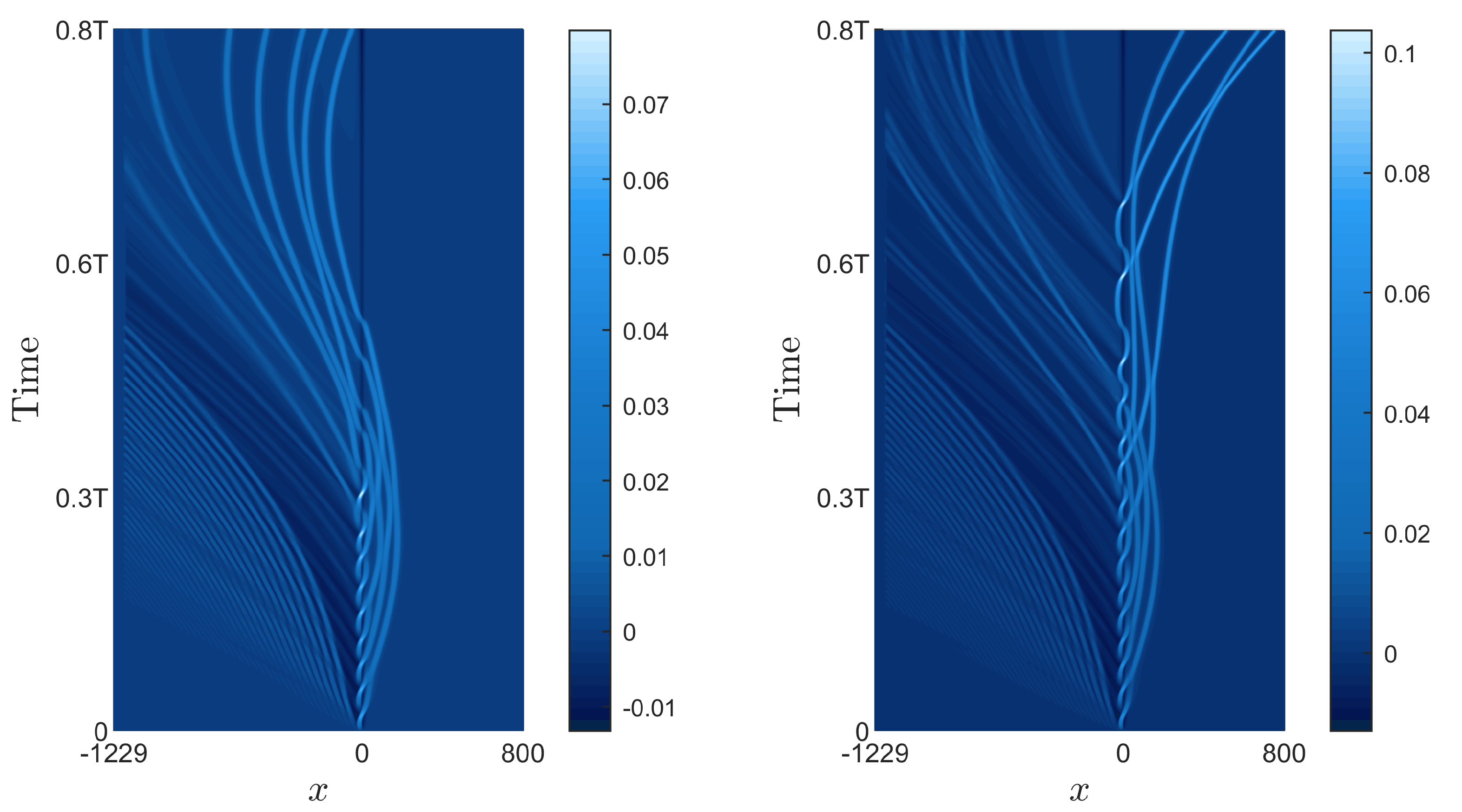
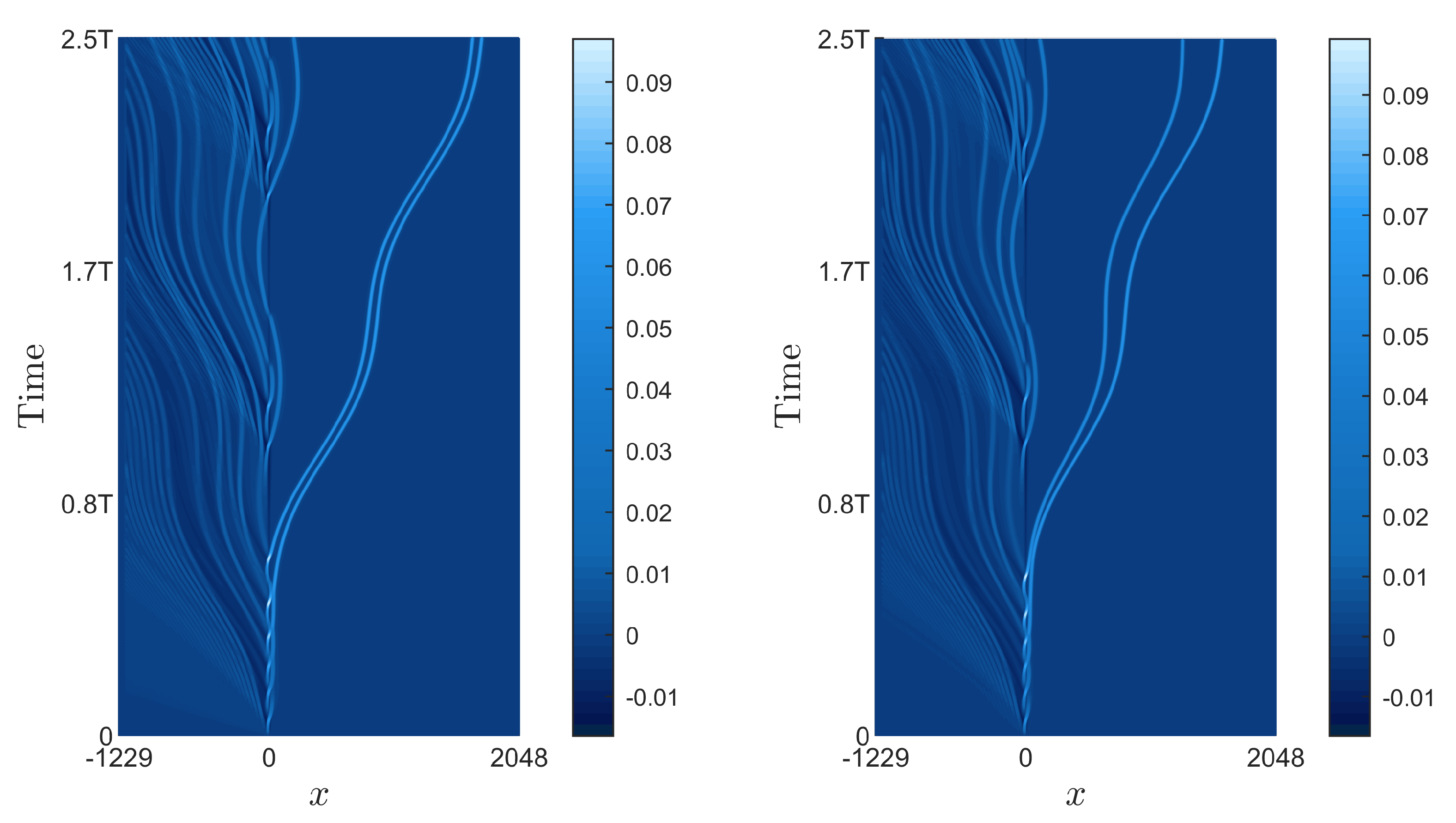
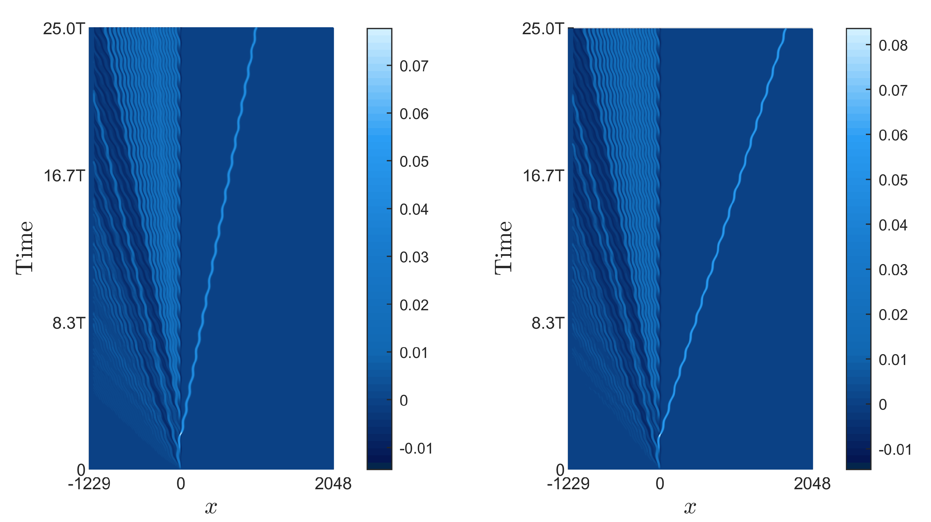
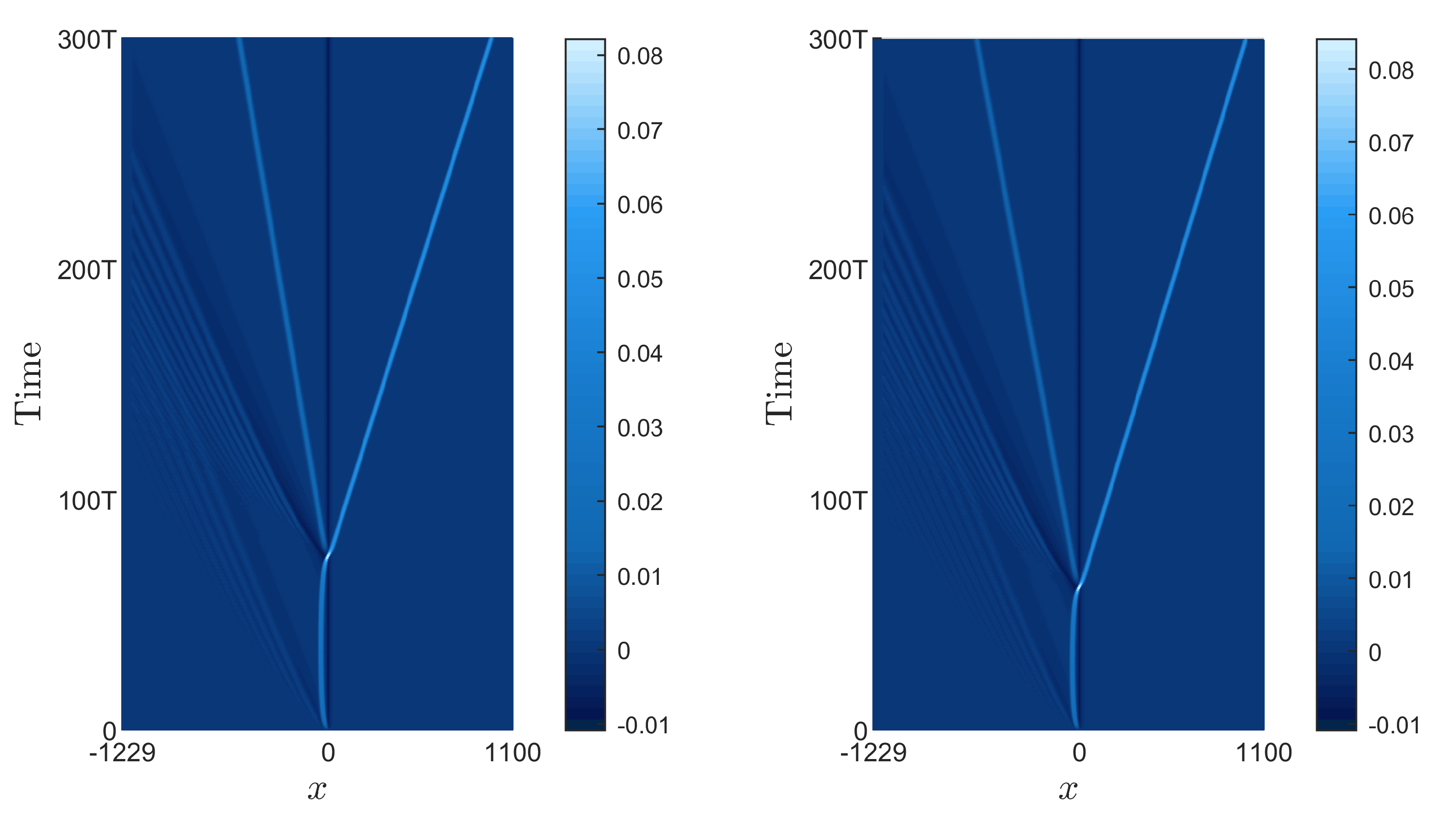
4. Results and Discussions

Previous studies have investigated the interaction between solitary waves and a localized external force that moves with variable speed and constant acceleration within the framework of the KdV equation [12,21,38] and the Whitham equation [32]. These authors identified specific parameter regimes wherein solitary waves are spontaneously generated and trapped by the external force. In the present work, we expand upon these findings by exploring the emergence of solitary trapped waves under an external force that moves with variable speed and non-constant acceleration.
The focus of this study is not an exhaustive analysis of trapped waves; rather, we present several illustrative examples to highlight the parametric regimes in which such waves are spontaneously generated. To this end, we select a fixed moving disturbance profile, defined as
P ( x ) = b sech 2 x 10 ,
and with variable speed
v ( t ) = v a cos θ t + v 0 .
To facilitate comparison between the constant acceleration case and the non-constant one, we set the initial speed v 0 = 0.05 , the disturbance amplitude b = 10 3 , and v a = 0.05 , as in the work of Flamarion [32]. We then vary the frequency parameter θ and denote the period of the speed ( 2 π / θ ) by T. The choice of parameters ensures that the speed is always non-positive.
Although we consider different values of the frequency parameter, due to the vast number of possible choices we only present those that yield qualitatively different dynamics in the free surface. Specifically, we select θ 0 in order to compare our results with the constant acceleration case reported by Flamarion et al. [38], and gradually increase the frequency thereafter.
In the first case, we set θ 1.75 × 10 4 (T = 36,000), which allows us to observe the periodic generation of solitary waves upstream along with small amplitude waves downstream, which is qualitatively similar to the constant speed case reported in [38]. At early times, both the KdV and Whitham equations generate solitary waves that do not move away from the external force. However, as time progresses, the solitary waves interact in different ways in each regime, leading to distinct dynamics. This behavior is depicted in Figure 1 and further detailed in Supplemental Video S1. The color code employed in this figure, as well as in the subsequent ones of similar nature, denotes the values of the wave u ( x , t ) at a specific position x and time t. Lighter and darker colors correspond to higher and lower values of u, respectively.
As we increase the frequency to θ 5.24 × 10 4 ( T = 12 , 000 ), the dynamics described in Figure 1 are no longer representative of the free surface. Instead, both the KdV and Whitham equations predict the generation of a pair of solitary waves propagating upstream. This behavior is shown in Figure 2 and Supplemental Video S2.
Unlike the previous cases, when θ 3.14 × 10 3 ( T = 2000 ), the period in which waves are generated is somewhat more regular and is similar to the period T of the speed. In the simulation depicted in Figure 3, the speed v ( t ) completes eleven cycles and eleven solitary waves are generated upstream. The profile of these waves is similar to the v = 0 case, as seen in detail in Supplemental Video S3. It is possible to observe differences in the speed of the upstream solitary waves between the Whitham and fKdV models, resulting in collisions between these waves at later times.
In contrast to the previous scenario, in which solitary waves are periodically generated upstream, only one solitary wave is observed upstream for θ 5.24 × 10 3 ( T = 1200 ). As shown in Figure 4 and Supplemental Video S4, the solitary wave travels slower in the fKdV model than in the Whitham model.
Finally, for θ 6.28 × 10 2 ( T = 100 ), small-amplitude waves are generated and propagate downstream, while large oscillations arise where the pressure is applied. As the amplitude reaches a critical value, the center oscillation breaks into two waves that propagate in opposite directions. This phenomenon is depicted in Figure 5 and Supplemental Video S5.
A query that naturally emerges relates to the nature of the waves produced in the scenario where the velocity v (defined in Equation (11)) is positive. Under such circumstances, the generated waves predominantly consist of a periodic wave train propagating both upstream and downstream in spite of the choice of the frequency θ .
To ensure confidence in the accuracy of our numerical method and the validity of our results, we present a resolution study. This study does not aim to provide an exhaustive analysis of resolution for each simulation discussed previously; rather, it serves to demonstrate that the wave profiles are accurately captured by different choices of Δ x . Therefore, we only carry out a resolution study for the case where θ = 3.14 × 10 3 , for which the wave dynamics are shown in Figure 3, and compute the distance between wave solutions for different values of Δ x .
We use the notation u Δ x ( t ) to refer to the wave profile at time t computed using a grid with size Δ x . To establish the accuracy of our numerical method and ensure the reliability of our results, we adopt a reference grid with grid size Δ x = 0.05 , which is the finest resolution we have computed. We denote by u ( t ) the wave profile computed using the reference grid.
Table 1 presents the results for both the fKdV and the Whitham equations. As shown in the table, the relative error decreases as the grid size is reduced. Therefore, it can be concluded that the numerical solutions presented in this study are independent of the spatial grid resolution.

5. Conclusions

In conclusion, this study presents a novel exploration of the appearance of solitary trapped waves in the presence of an external force with variable speed and non-constant acceleration. Our numerical simulations can provide insights into the main properties of these waves, and reveal a nonlinear relationship between the number of generated waves and the speed period. Moreover, the identification of diverse regimes suggests the possibility of chaos, which highlights the need for further investigation of Lyapunov exponents.
The implications of this study extend beyond the field of water wave theory, and can motivate further research in other physical scenarios; examples include the investigation of external forces with variable speed and non-constant acceleration in surface waves in electric normal fields, wind waves, atmospheric waves, and elastic waves in solids.

Supplementary Materials

The following supporting information can be downloaded at: https://www.mdpi.com/article/10.3390/fluids1010000/s1.

Author Contributions

Conceptualization: M.V.F., R.R.-J., D.L.S.S.V. and A.M.S.; Methodology, Analysis, and Writing: M.V.F., R.R.-J., D.L.S.S.V. and A.M.S. All authors have read and agreed to the published version of the manuscript.

Funding

Author A.M.S. is grateful for the financial support provided by the CAPES Foundation (Coordination for the Improvement of Higher Education Personnel) during part of the development of this work.

Institutional Review Board Statement

Not applicable.

Informed Consent Statement

Informed consent was obtained from all subjects involved in the study.

Data Availability Statement

Not applicable.

Acknowledgments

M.V.F. and R.R.J. are grateful to IMPA for hosting them as visitors during the 2023 Post-Doctoral Summer Program. The authors would like to thank the reviewers for their comments and constructive criticism that helped us to improve the presentation of this work.

Conflicts of Interest

The authors declare no conflict of interest.

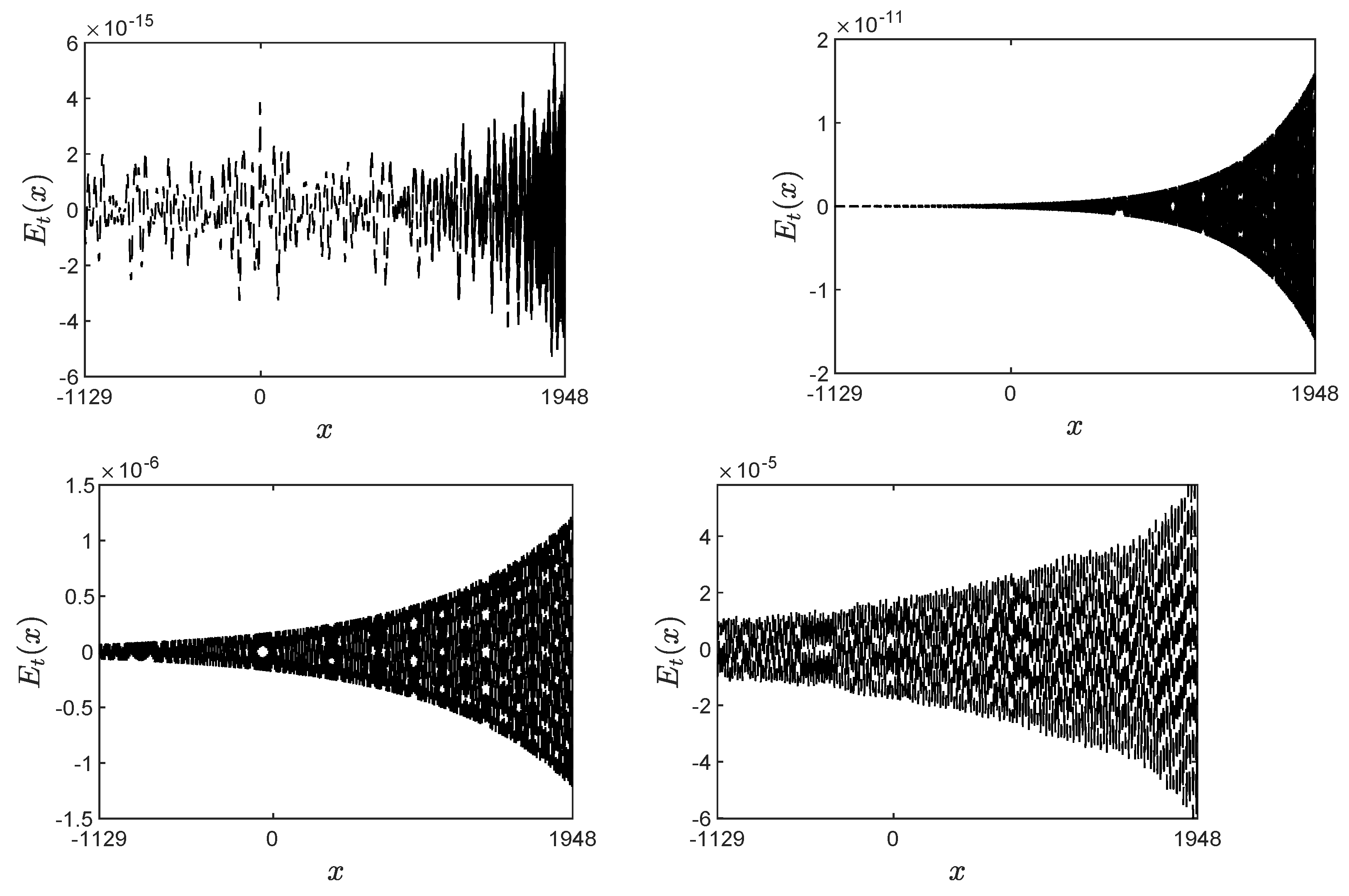
Appendix A. The Sponge Layer Effect

In this section, a comparative study is presented between the solutions of the forced Korteweg–de Vries (fKdV) equation with and without the implementation of the sponge layer. The simulation is carried out with the parameters Δ x = 0.2 , Δ t = 0.01 , θ = 5.24 × 10 4 ; the solution without the sponge layer is computed with N = 2 15 , while with the sponge layer it is computed with N = 2 14 . As elaborated in Section 3, these parameters lead to a computational domain that is half the size of the domain without the sponge layer.
To demonstrate the efficiency of the sponge layer approach, the quantity
E t ( x j ) = u ( x j , t ) u s ( x j , t )
is monitored, where u and u s are the solutions of the fKdV Equation (7) without and with sponge layer, respectively, and x j are the common points between the two grids. The results are depicted in Figure A1. It can be observed that the difference between the solutions is negligible. Therefore, the sponge layer represents a valid artificial technique that can be employed to reduce computational costs when running simulations over extended periods.
When applied to the Whitham equation, the analysis of the sponge layer presented above yields analogous results. Thus, to avoid repetition, we have omitted the figures on this topic.
Figure A1. Comparison between the solutions of the fKdV equation with and without the sponge layer at t = 500 , t = 1000 , t = 5000 and t = 15,000 (from top to bottom), where E t ( x ) = u ( x , t ) u s ( x , t ) and where u and u s are the solution of the fKdV equation (7) without and with the sponge layer, respectively.
Fluids 08 00223 g0a1

References

  1. Craik, A.D.D. The Origins of water Wave Theory. Annu. Rev. Fluid Mech. 2004, 36, 1–28. [Google Scholar] [CrossRef]
  2. Zabusky, N.J.; Kruskal, M.D. Interaction of solitons in a collisionless plasma and the recurrence of initial states. Phys. Rev. Lett. 1965, x15, 240. [Google Scholar] [CrossRef] [Green Version]
  3. Manukure, S.; Booker, T. A short overview of solitons and applications. Partial. Differ. Equations Appl. Math. 2021, 4, 100140. [Google Scholar] [CrossRef]
  4. Joseph, A. Investigating Seafloors and Oceans: From mud Volcanoes to Giant Squid; Elsevierl: Amsterdam, The Netherlands, 2016. [Google Scholar]
  5. Baines, P. Topographic Effects in Stratified Flows; Cambridge University Press: Cambridge, UK, 1995. [Google Scholar]
  6. Johnson, R.S. Models for the formation of a critical layer in water wave propagation. Philos. Trans. R. Soc. Math. Phys. Eng. Sci. 2012, 370, 1638–1660. [Google Scholar] [CrossRef] [PubMed]
  7. Ermakov, A.; Stepanyants, Y. Soliton interaction with external forcing within the Korteweg-de Vries equation. Chaos 2019, 29, 013117. [Google Scholar] [CrossRef] [Green Version]
  8. Flamarion, M.V.; Ribeiro, R., Jr. Solitary water wave interactions for the Forced Korteweg-de Vries equation. Comp. Appl. Math. 2021, 40, 312. [Google Scholar] [CrossRef]
  9. Grimshaw, R.; Malewoong, M. Transcritical flow over two obstacles: Forced Korteweg-de Vries framework. J. Fluid Mech. 2016, 809, 918–940. [Google Scholar] [CrossRef]
  10. Grimshaw, R.; Malewoong, M. Transcritical flow over obstacles and holes: Forced Korteweg-de Vries framework. J. Fluid Mech. 2019, 881, 660–678. [Google Scholar] [CrossRef]
  11. Grimshaw, R.; Pelinovsky, E.; Tian, X. Interaction of a soliton with an external force. Physica D 1994, 77, 405–433. [Google Scholar] [CrossRef]
  12. Grimshaw, R.; Pelinovsky, E.; Sakov, P. Interaction of a soliton with an external force moving with variable speed. Stud. Appl. Math. 1996, 142, 433–464. [Google Scholar]
  13. Kim, H.; Choi, H. A study of wave trapping between two obstacles in the forced Korteweg-de Vries equation. J. Eng. Math. 2018, 108, 197–208. [Google Scholar] [CrossRef]
  14. Lee, S.; Whang, S. Trapped supercritical waves for the forced KdV equation with two bumps. Appl. Math. Model. 2015, 39, 2649–2660. [Google Scholar] [CrossRef]
  15. Lee, S. Dynamics of trapped solitons for the forced KdV equation. Symmetry 2018, 10, 129. [Google Scholar] [CrossRef] [Green Version]
  16. Malomed, B.A. Emission of radiation by a KdV soliton in a periodic forcing. Phys. Lett. A 1993, 172, 373–377. [Google Scholar] [CrossRef]
  17. Flamarion, M.V. Generation of trapped depression solitons in gravity-capillary flows over an obstacle. Comp. Appl. Math. 2022, 41, 31. [Google Scholar] [CrossRef]
  18. Flamarion, M.V.; Ribeiro, R., Jr. Gravity-capillary flows over obstacles for the fifth-order forced Korteweg-de Vries equation. J. Eng. Math. 2021, 129, 1–17. [Google Scholar] [CrossRef]
  19. Flamarion, M.V.; Pelinovsky, E. Solitary wave interactions with an external periodic force: The extended Korteweg-de Vries framework. Mathematics 2022, 10, 4538. [Google Scholar] [CrossRef]
  20. Flamarion, M.V.; Pelinovsky, E. Soliton interactions with an external forcing: The modified Korteweg–de Vries framework. Chaos Solitons Fractals 2022, 165, 112889. [Google Scholar] [CrossRef]
  21. Grimshaw, R.; Pelinovsky, E. Interaction of a soliton with an external force in the extended Korteweg-de Vries equation. Int. J. Bifurcat. Chaos 2002, 12, 2409–2419. [Google Scholar] [CrossRef]
  22. Pelinovsky, E. Autoresonance Processes under Interaction of Solitary Waves with the External Fields. Int. J. Fluid Mech. Res. 2002, 30, 493–501. [Google Scholar] [CrossRef]
  23. Whitham, G.B. Linear and Nonlinear Waves; John Wiley & Sons Inc: New York, NY, USA, 1974. [Google Scholar]
  24. Whitham, G.B. Variational methods and applications to water waves. Phil. Trans. R. Soc. A 1967, 229, 6–25. [Google Scholar]
  25. Ehrnström, M.; Kalisch, H. Traveling waves for the Whitham equation. Differ. Integral Equ. 2009, 22, 1193–1210. [Google Scholar] [CrossRef]
  26. Ehrnström, M.; Wahlén, E. On Whitham’s conjecture of a highest cusped wave for a nonlocal dispersive equation. Ann. L’Institut Henri Poincaré C 2019, 36, 769–799. [Google Scholar]
  27. Hur, V.M.; Pandey, A.K. Modulational instability in a full-dispersion shallow water model. Stud. Appl. Math. 2019, 142, 3–47. [Google Scholar] [CrossRef] [Green Version]
  28. Sanford, N.; Kodama, K.; Clauss, G.F.; Onorato, M. Stability of traveling wave solutions to the Whitham equation. Phys. Lett. A 2014, 378, 2100–2107. [Google Scholar] [CrossRef]
  29. Klein, C.; Linares, F.; Pilod, D.; Saut, J.C. On Whitham and Related Equations. Stud. Appl. Math. 2018, 140, 133–177. [Google Scholar] [CrossRef] [Green Version]
  30. Carter, J.D.; Kalisch, H.; Kharif, C.; Abid, M. The cubic vortical Whitham equation. arXiv 2021, arXiv:2110.02072v1. [Google Scholar] [CrossRef]
  31. Grimshaw, R.; Malomed, B.A.; Tian, X. Dynamics of a KdV soliton due to periodic forcing. Phys. Lett. A 1993, 179, 291–298. [Google Scholar] [CrossRef]
  32. Flamarion, M.V. Trapped waves generated by an accelerated moving disturbance for the Whitham equation. Partial. Differ. Equ. Appl. Math. 2022, 5, 100356. [Google Scholar] [CrossRef]
  33. Grimshaw, R.; Pelinovsky, E.; Talipova, T.; Kurkina, O. Internal solitary waves: Propagation, deformation and disintegration. Nonlin Processes. Geophys. 2010, 17, 633–649. [Google Scholar] [CrossRef] [Green Version]
  34. Chen, M. Equations for bi-directional waves over an uneven bottom. Math. Comput. Simul. 2003, 62, 3–9. [Google Scholar] [CrossRef]
  35. Aceves-Sánchez, P.; Minzoni, A.A.; Panayotaros, P. Numerical study of a nonlocal model for water- waves with variable depth. Wave Motion. 2013, 50, 80–93. [Google Scholar] [CrossRef]
  36. Vargas-Magaña, R.M.; Marchant, T.R.; Smyth, N.F. Numerical and analytical study of undular bores governed by the full water wave equations and bidirectional Whitham-Boussinesq equations. Phys. Fluids 2021, 33, 067105. [Google Scholar] [CrossRef]
  37. Carter, J.D. Bidirectional Whitham equations as models of waves on shallow water. Wave Motion 2018, 82, 5161. [Google Scholar] [CrossRef]
  38. Flamarion, M.V.; Milewski, P.A.; Nachbin, A. Rotational waves generated by current-topography interaction. Stud. Appl. Math. 2019, 142, 433–464. [Google Scholar] [CrossRef]
  39. Milewski, P.A. The Forced Korteweg-de Vries equation as a model for waves generated by topography. CUBO Math. J. 2004, 6, 33–51. [Google Scholar]
  40. Trefethen, L.N. Spectral Methods in MATLAB; SIAM: Philadelphia, PA, USA, 2001. [Google Scholar]
  41. Alias, A.; Ismail, N.N.A.N.; Harun, F.N. Pseudospecteral method with linear damping effect and de-aliasing technique in solving nonlinear PDEs. J. Physics Conf. Ser. 2019, 1366, 012009. [Google Scholar] [CrossRef] [Green Version]
Figure 1. Blue-scale plot of the generated waves for the fKdV equation (left) and Whitham equation (right) for θ 1.75 × 10 4 (T = 36,000).
Fluids 08 00223 g001
Figure 2. Blue-scale plot of the generated waves for the fKdV equation (left) and Whitham equation (right) for θ 5.24 × 10 4 (T = 12,000).
Fluids 08 00223 g002
Figure 3. Blue-scale plot of the generated waves for the fKdV equation (left) and Whitham equation (right) for θ 3.14 × 10 3 ( T = 2000 ).
Fluids 08 00223 g003
Figure 4. Blue-scale plot of the generated waves for the fKdV equation (left) and Whitham equation (right) for θ 5.24 × 10 3 ( T = 1200 ).
Fluids 08 00223 g004
Figure 5. Blue-scale plot of the generated waves for the fKdV equation (left) and Whitham equation (right) for θ 6.28 × 10 2 ( T = 100 ).
Fluids 08 00223 g005
Table 1. Resolution study for the wave generated with T = 2000 .
N Δ x
max t [ 0 , 6000 ] u Δ x ( t ) u ( t ) 2 u ( · , t ) 2
Equation
2 13 0.4 3.62 × 10 8 fKdV
8.08 × 10 8 Whitham
2 14 0.2 2.65 × 10 12 fKdV
3.11 × 10 13 Whitham
2 15 0.1 8.85 × 10 13 fKdV
2.12 × 10 13 Whitham
Disclaimer/Publisher’s Note: The statements, opinions and data contained in all publications are solely those of the individual author(s) and contributor(s) and not of MDPI and/or the editor(s). MDPI and/or the editor(s) disclaim responsibility for any injury to people or property resulting from any ideas, methods, instructions or products referred to in the content.

