
Comprehensive Perturbation Approach to Nonlinear Viscous Gravity–Capillary Surface Waves at Arbitrary Wavelengths in Finite Depth
Department of Theoretical Physics, Institute of Physics, Eötvös Loránd University, Pázmány Péter sétány 1/A, 1117 Budapest, Hungary
*
Author to whom correspondence should be addressed.
Fluids 2023, 8(8), 218; https://doi.org/10.3390/fluids8080218
Submission received: 21 June 2023
/
Revised: 19 July 2023
/
Accepted: 25 July 2023
/
Published: 27 July 2023
Abstract
:This study presents a comprehensive analysis of the second-order perturbation theory applied to the Navier–Stokes equations governing free surface flows. We focus on gravity–capillary surface waves in incompressible viscous fluids of finite depth over a flat bottom. The amplitude of these waves is regarded as the perturbation parameter. A systematic derivation of a nonlinear-surface-wave equation is presented that fully takes into account dispersion, while nonlinearity is included in the leading order. However, the presence of infinitely many over-damped modes has been neglected and only the two least-damped modes are considered. The new surface-wave equation is formulated in wave-number space rather than real space and nonlinear terms contain convolutions making the equation an integro-differential equation. Some preliminary numerical results are compared with computational-modelling data obtained via open source CFD software OpenFOAM.
PACS:
47.10.-g; 47.11.-j1. Introduction
A great number of studies have been conducted on gravity–capillary surface waves and there have been notable advancements in the study of nonlinear and dispersive gravity–capillary surface waves, with a particular focus on the effect of viscosity [1,2,3,4,5,6,7,8,9,10,11]. Several linear and weakly nonlinear equations have been suggested to represent the propagation of surface waves and dispersion relations [11,12,13,14]. The study of the nonlinear properties of capillary–gravity waves in infinitely deep water was initiated by Harrison [15] using a perturbation expansion. Harrison [15] focused on the influence of viscosity and surface tension. The author considered these parameters but did not provide an exact linear-dispersion relation. He found that the second approximations to both the velocity potential and the free-surface profile contained singularities for particular combinations of the reduced tension, gravity and wavelength.
As for the non-viscous case, the interested reader is referred to the excellent literature review article of Dias and Kharif [16]. Two-dimensional progressive gravity–capillary waves can also be studied at the interface between two fluids of different densities [17]. Hunt applied the Levi–Civita method for progressive and standing interface waves and obtained formulae of the wave profile and phase velocity up to the third order. In that paper, finite-depth fluid was studied. The author did not consider viscosity or surface tension and did not provide an exact linear-dispersion relation. Tsuji and Nagata [18] investigated the impact of surface tension in a scenario where deep and inviscid fluid was considered. They did not provide an exact linear-dispersion relation but contributed to the understanding of the role of surface tension in wave propagation, particularly in the absence of other parameters. They used a perturbation expansion in wave amplitude to the fifth order, for interfacial gravity waves of infinite depths. Their results suggested that the maximum value of the wave steepness may be limited by shear instability at the interface rather than the breaking condition at the interface. Matsuno [1,2] derived a Boussinesq-type model through an expansion in a steepness parameter , where a represents the amplitude scale and l represents the wavelength scale. The author demonstrated that an appropriate extension of the integral kernel [19,20] establishes a connection with basic propagation models, such as the nonlinear Schrodinger equation (NLS) [21] and its variations (modified NLS—MNLS), with the most prominent being the Dysthe equation [22]. He pursued the perturbation analysis to the fourth order in wave steepness. One of the main effects at this order in infinite depth is precisely the influence of the wave-induced mean flow.
Viscosity serves as a pervasive damping mechanism [23,24], alongside other dissipation pathways such as impurities, obstacles and wave breaking. Its significance extends to the fundamental investigations of gravity waves [2,6,12,25]. More recently, a model for viscous deep-water waves was proposed by Dias, Dyachenko and Zakharov [26]. However, surface-tension effects have been neglected. The authors did not provide an exact linear-dispersion relation but their study enhanced the understanding of the influence of viscosity on nonlinear-wave behavior. In 2013, Liu, Hwung and Yang [27] considered the case of a two-fluid system with free surface. Second-order solutions were obtained, using the perturbation method. In cases of low viscosity, the vorticity is primarily concentrated within a narrow boundary layer in close proximity to the surface, as noted in previous studies [23,24,28,29]. Moreover, a multitude of authors have made significant contributions to comprehending the dispersion mechanism, wave propagation and stability analysis of capillary–gravity waves in finite depth [5,12,13,30,31,32,33].
In order to investigate the nonlinearities for surface water waves, Le Meur applied the Boussinesq approximation, which relates the amplitude (A), fluid depth (h) and wavelength (l)) as . This condition together with the assumption of a large Reynolds number led to the separate treatment of the boundary layer from the bulk of the fluid [34]. Le Meur derived the exact dispersion relation in the linear regime, considering surface tension and viscosity effects in a viscous fluid of finite depth [33,34]. He concluded that for a large Reynolds number, represents the case of interest where viscous and gravitational effects balance.
The impact of viscosity on the nonlinear propagation of surface waves at the interface of air and a fluid of large depth is discussed in [35]. They proposed modified hydrodynamic boundary conditions to model both short and long waves. They showed that the linearity plays the main role in both gravity and capillary–gravity waves while the nonlinearity represents only small corrections. In the limit of infinite depth, authors utilized the exact linear-dispersion relation
where denotes the kinematic viscosity of the fluid and . stands for surface tension. Ghahraman and Bene [33] conducted an analysis of the linear dispersion relation in an unbounded channel with uniform depth, without imposing any constraints on the parameters. The authors focused on investigation of the conditions of wave propagation in the presence of viscosity and surface tension. It is discovered that both very short and very long waves are prohibited from propagating in thicker fluid layers, while the presence of two distinct length scales related to viscosity and surface tension is observed. Their findings indicate that there is a countably infinite number of modes present at any given horizontal wave number, but only those with the lowest damping rate are capable of describing propagating modes (see details in Section 3, after Equation (36)). All the other modes are over-damped. Further, in a fluid layer of sufficiently small thickness, there is a complete absence of wave propagation. Retaining the two modes with the least damping, a bidirectional evolution equation,
may be written down [33] for surface elevation , where k denotes the horizontal wave number. It is a linear second-order differential equation at each wave number k and is applicable regardless of the feasibility of propagation. Note that and stand for the complex angular frequencies of the two modes.
Surface waves are typically nonlinear. When nonlinearity is factored in, it may stimulate previously dormant linear modes, potentially resulting in enhanced attenuation if the secondary modes are over-damped or, conversely, propagating the appearance if the primary modes are over-damped but the secondary modes are under-damped. Such impacts would not be anticipated under a linear approximation. Several intricate behaviors such as frequency modulation, wave mixing and mode generation, solitons, breeders, nonlinear resonances and modulational instabilities may emerge due to nonlinearity in wave equations, predominantly in non-dissipative cases. It is expected that these phenomena persist in some form even when dissipation is present, thereby driving the need for an effective tool to scrutinize these effects.
It is intriguing what the interplay is between dispersion, dissipation and nonlinearity. For instance, by considering the simplified nonlinear-wave equation
it is well known what happens if one or more of these factors are absent. When the second derivative (representing dissipation) is removed, the Korteweg–de Vries (KdV) equation, a well-established solitonic solution, arises. A scenario without the third derivative term (denoting dispersion) leads to an equation where dissipation instigates concurrent decay and wave-profile broadening, with nonlinearity engendering asymmetry in the wave profile. Nevertheless, the picture becomes less discernible when all three aspects are in operation. Moreover, it is also a question what the correct nonlinear-wave equation is for capillary–gravity waves. Extant literature largely relies on approximations such as the Boussinesq approximation. This research aims to present a tool by introducing a method that incorporates nonlinear terms to a leading order without depending on such approximations.
This paper aims to generalize the results of [33], especially Equation (2), by including the leading nonlinear terms in the Navier–Stokes equation, as well as boundary conditions. In order to achieve this objective, we employ a perturbative approach to solve the Navier–Stokes equations for the surface-wave problem up to the second order, where the wave amplitude is considered to be a small parameter. This method allows for the systematic study of nonlinearity in various fluid phenomena [36,37,38,39,40,41,42,43]. At this stage, the calculation is still completely general; in particular, all the modes are included. Then, we look for a generalization of Equation (2). We write down the most general quadratic second-order differential equation that is allowed via horizontal translational symmetry. We solve this equation perturbatively to the second order and then compare the result with that of the previous perturbation theory of surface waves, where we keep only the two least-damped modes. This comparison results in a well-defined nonlinear integro-differential equation for surface elevations that is self-consistent. Incorporating further modes would lead to the emergence of time derivatives of a higher order than two, a feature that is also observed at the linear level. Table 1 presents a summary and comparison of the existing literature with regards to their parameters, dispersion relations and the methodologies employed. Based on the findings presented in Table 1, only the works conducted by Le Meur [34] and Ghahraman and Bene [33] derive an exact linear-dispersion relation for finite fluid depth in the presence of viscosity, gravity and surface tension. In contrast, the present study explores nonlinearity without resorting to any further approximation or restriction than the smallness of the wave amplitude, distinguishing it from Le Meur’s methodology.
The plan of the paper is as follows. In Section 2, a formulation of the problem is given. First-order and second-order approximations are discussed in Section 3 and Section 4, respectively. In Section 5, we derive the surface-wave equation based on perturbation theory. The results are summarized and discussed in the concluding section, Section 6. Some longer expressions are relegated to the Appendix A.
2. Formulation of the Problem
Consider the irrotational flow of an incompressible inviscid fluid with a free surface. A Cartesian coordinate system is adopted, with the x-axis located on the still-water plane and with the z-axis pointing vertically upwards. The fluid domain is bounded by the bed at and the free surface at (Figure 1). The Navier–Stokes (NS) equations in the bulk are:
Since the right-hand side is a full gradient, we have
with bottom boundary conditions
and horizontal and vertical components of net force at the surface (up to second-order precision in amplitudes):
Further, we have the kinematic condition for the surface
By eliminating the pressure from Equations (6) and (7) with the help of the Navier–Stokes equations, we have the following equations, respectively.
Assuming incompressible fluid, we may express the velocity components in terms of the stream function as
Inserting Equations (11) and (12) into the previous equations, we obtain
in the bulk and
at the bottom (). The surface boundary conditions are (at ):
and
We are looking for a solution in a form
where the superscript refers to the order.
3. First-Order Solutions
Inserting decompositions (19) and (20) into the equations, we have in the first order
in the bulk (),
at the bottom () and
on the surface ().
Generally, the first-order solution is an integral over wave number k.
where and
The angular frequency reads
Modes are labelled by horizontal wave number k (a continuous parameter) and discrete values which are solutions of the following equation [33,44]
Here
Figure 2 demonstrates that a large number of solutions to Equation (32) are achieved by setting constant parameters and generating branches that alter as K changes. The imaginary parts of the frequencies are displayed. Nonzero real parts appear when two branches merge [33]. Only the lowest two branches are displayed in Figure 3, both the real and imaginary parts of the frequencies. At this parameter setting, there is a broader range of wave numbers where propagation of waves is possible.
Summation in (27) and (28) is understood over the possible branches (denoted by bracketed upper indices) of the dispersion relation . Note that if is a solution, so is at the same k value, though it may yield a different branch. The branches of the dispersion relation at k are the same as at . This allows indexing in the following way:
Thus, we have
Since the coefficients always appear in the combination , henceforth we shall denote this sum with , satisfying . Note that may be expressed in terms of the spatial Fourier transform of the initial conditions and , if we keep just two branches of the dispersion relation.
4. Second-Order Solutions
In second-order approximation, the main system of equations are
in the bulk and
at the bottom (). The surface boundary conditions are (at ):
and
The second-order calculation requires evaluation of the right-hand side of Equation (40), which is quadratic in ; therefore, one obtains a double integral. Explicitly, we obtain for the right-hand side of Equation (40)
Note that . Other coefficients depend on both and (see Appendix A). The solution of (40) can be written in a similar form:
Here again . Other coefficients can be calculated directly from Equation (40) (see Appendix A). The homogeneous part is written as
where
Coefficients are to be determined from boundary conditions (41)–(45). Bottom boundary conditions (41) and (42) yield the equations
and
respectively. Surface boundary condition (43) determines as
Here, is a function of both and ; its explicit expression is lengthy and is given therefore as a Appendix A item. Equations (44) and (45) combined with Equations (50)–(52) provide us with the relations
and
respectively. The right-hand sides , no longer contain any unknowns; they are well-determined functions of and . Their explicit expressions are again given as a Appendix A item.
Solving Equations (50), (51), (53) and (54) we obtain finally
where stands for the second line of Equation (52).
5. Surface-Wave Equation
Equations (28) and (55) yield the solution for the surface shape up to the second order. We discuss now whether and how one can derive a single wave equation for the surface shape to this order, without reference to the underlying bulk Navier–Stokes equations. Provided that we keep only a single pair of values of the dispersion relation, this equation—due to translation symmetry—in k-space must have the form
where functions , and are symmetric, while is antisymmetric with respect to the exchange of their variables:
Alternatively, one may write
where
We show how the two-variate functions may be determined if is known. The idea is to solve (56) perturbatively and compare the result with Equation (55). The first-order solution of (56) coincides with the spatial Fourier transform of Equation (39),
where
Certainly, the expression of the coefficients is arbitrary, so the specific form (61) may be chosen without restricting generality. It is suitable for making contact with the previous calculations.
The second-order solution satisfies
The homogeneous part of the solution may be included in the first-order solution; hence, it suffices to construct the particular solution with the same time dependence as the correction term, i.e.,
which is identical with Equation (55). Upon inserting Equations (60) and (63) into Equation (62), we have
where
Note that is independent of and , due to (61). Since branch indices a and b can be both either 1 or 2, the set of equations (64) can be solved for any given k and values:
With this, Equation (58) is completely defined.
6. Numerical Results
As reference, computational modelling was utilized to simulate the physical problem under consideration. The computational simulations were executed via the open-source computational fluid dynamics (CFD) software, OpenFOAM. This platform offered an efficient and highly versatile framework for testing the varied parameters that impact the problem. The geometry is a two-dimensional rectangular configuration, as shown in Figure 4. Our simulations accounted for several depths that corresponded to both propagation and non-propagation modes for glycerine in the presence of viscosity and surface tension, enabling a comprehensive understanding of the surface-wave propagation. In addition, we considered both linear and nonlinear regimes, thus broadening our approach to investigate the first- and the second-order solutions.
The chosen solver for our simulations was inteFoam, recognized for its suitability in handling free-surface flow problems. The computational domain was a box of dimensions one cubic meter. This size was deemed appropriate for capturing the key phenomena without imposing prohibitive computational demands. The initial wave profile used in our simulations was a Gaussian wave packet, selected for its ability to represent a localized disturbance while maintaining a continuous and differentiable waveform.
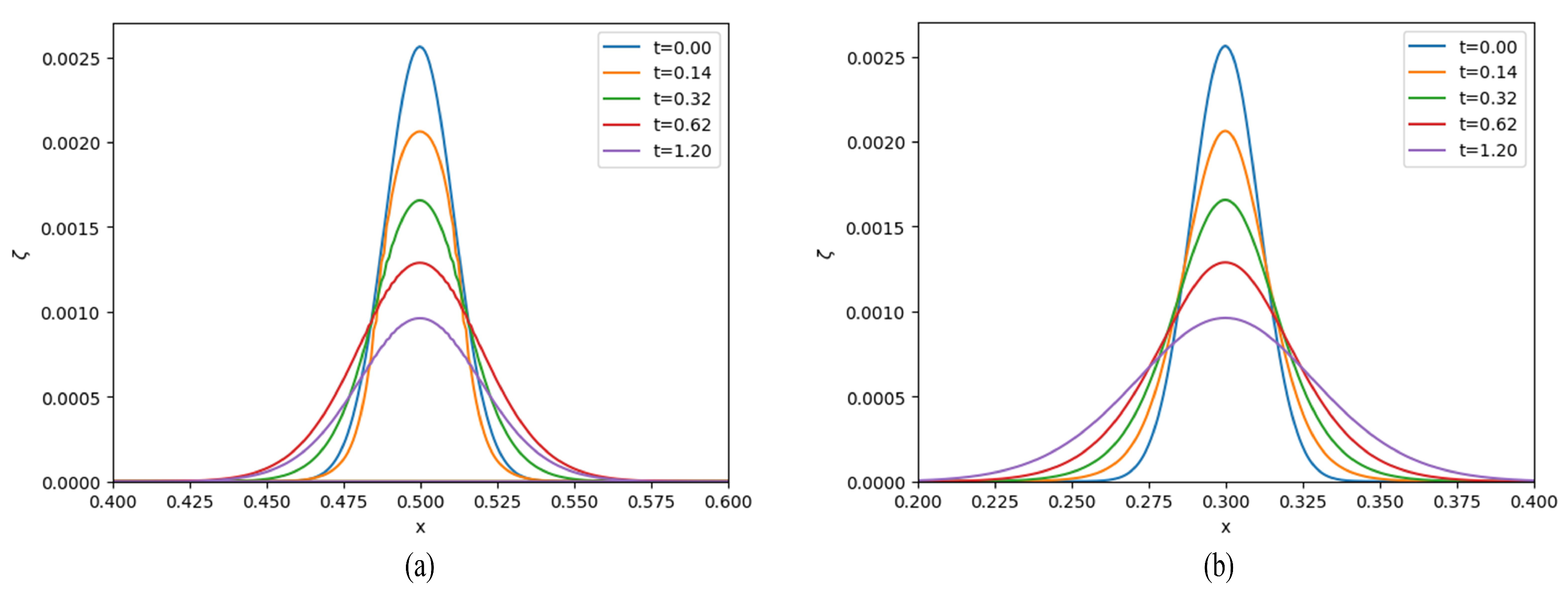
In the linear regime, we set the wave amplitude to of the depth. As illustrated in Figure 5, this configuration confirmed the linear behaviour as discussed in [33]. On the other hand, for the nonlinear regime, the wave amplitude was set to half the depth. This resulted in the formation of a double hump, a characteristic feature corresponding to the second-order approximation. The observation of this feature provided an affirmation of the nonlinear dynamics inherent in our theoretical approach and simulation model. Hence, through the use of OpenFOAM and the specific simulation parameters, our study supports the second-order perturbative-approach theory, providing a comprehensive understanding of the capillary–gravity surface wave propagation.
7. Conclusions
This work presents a novel tool, the surface-wave equation, Equation (58), developed specifically for investigating the complex interplay between nonlinearity, dispersion and dissipation. While this equation is exact in the absence of nonlinear terms, the novelty lies in the inclusion of these nonlinear terms, underscoring the importance of nonlinearity in the overall framework.
Second-order perturbation theory of the Navier–Stokes equations for free-surface flows was presented, with wave amplitude considered as the perturbation parameter. The results allowed a systematic derivation of a nonlinear-surface-wave equation. To this end, the most general quadratic second-order differential equation permissible under horizontal translational symmetry was formulated. It contains four unknown functions. Then, perturbation theory up to the second order is applied to this equation. This solution is compared with that of the previous perturbation theory applied to Navier–Stokes equations. This comparison allows for the determination of the four previously unknown functions.
No assumptions concerning the wavelength-to-layer-width ratio were made. Hence, the equation takes into account linear dispersion fully, while nonlinearity is included in leading order.
It should be noted that while the concept presented here can be extended to higher orders, one limitation is that we have neglected the presence of the infinitely many over-damped modes and kept only the two least-damped ones. Due to nonlinear coupling among the modes, this means that our equation may lead initially, when nonlinearity is significant, to somewhat slower decay than in reality. The extent of this should be still estimated.
The results contain rather long expressions that are difficult to handle. Therefore, discussion of special cases—like weakly damped waves—requires further efforts and is beyond the scope of the present paper. A further important open question is how our equation can be solved in a numerically effective way. Note that nonlinear dispersion relations remain outside the scope of this investigation as the surface-wave equation lacks an analytical solution.
Surface waves exhibit inherent nonlinearity, which can activate dormant linear modes and lead to enhanced attenuation if the secondary modes are over-damped. Conversely, if the primary modes are over-damped and the secondary modes are under-damped, nonlinearity may propagate their appearance. These effects are not expected within a linear approximation, highlighting the significance of considering nonlinearity when analyzing surface-wave behavior. Nonlinearity in wave equations can cause a variety of complex phenomena, including frequency modulation, wave mixing and mode formation, solitons, breeders, nonlinear resonances and modulational instabilities. These events are expected to remain in some form even when dissipation is present.
With regards to applications, the most intriguing circumstances involve strong nonlinearity coupled with weak dissipation. Despite this, this study investigates situations with weak nonlinearity and arbitrary dissipation, primarily excited by intellectual curiosity and a desire to define solitons amidst dissipation. This parameter setting can have direct application when examining highly viscous fluids such as oil and even in the studies involving freezing thick fluids [45].
Author Contributions
Methodology, A.G. and G.B.; Validation, G.B.; Formal analysis, A.G. and G.B.; Investigation, A.G. and G.B.; Writing—original draft, A.G.; Writing—review & editing, A.G. and G.B.; Supervision, G.B. All authors have read and agreed to the published version of the manuscript.
Funding
This research received no external funding.
Acknowledgments
This research was supported by the Ministry of Culture and Innovation and the National Research. A.G. greatly acknowledges the support from Stipendium Hungaricum No. 228712. We are indebted to our reviewers for their many helpful comments and suggestions.
Conflicts of Interest
The authors declare no conflict of interest.
Appendix A
Coefficients in Equation (46):
References
- Matsuno, Y. Nonlinear evolutions of surface gravity waves on fluid of finite depth. Phys. Rev. Lett. 1992, 69, 609. [Google Scholar] [CrossRef] [PubMed] [Green Version]
- Artiles, W.; Nachbin, A. Nonlinear evolution of surface gravity waves over highly variable depth. Phys. Rev. Lett. 2004, 93, 234501. [Google Scholar] [CrossRef] [PubMed] [Green Version]
- Wang, Z.; Milewski, P.A. Dynamics of gravity–capillary solitary waves in deep water. J. Fluid Mech. 2012, 708, 480–501. [Google Scholar] [CrossRef] [Green Version]
- Belibassakis, K.; Touboul, J. A nonlinear coupled-mode model for waves propagating in vertically sheared currents in variable bathymetry—Collinear waves and currents. Fluids 2019, 4, 61. [Google Scholar] [CrossRef] [Green Version]
- Gao, T.; Milewski, P.; Wang, Z. Capillary–gravity solitary waves on water of finite depth interacting with a linear shear current. Stud. Appl. Math. 2021, 147, 1036–1057. [Google Scholar] [CrossRef]
- Li, Y. A Mathematical Model for Nonlinear Gravity–Capillary Waves in a Large Temporal-Spatial Domain. In Porceedings of the EGU General Assembly 2023, Vienna, Austria, 24–28 April 2023; 2023. EGU23-13972. [Google Scholar]
- Ambrose, D.; Bona, J.; Nicholls, D. Well-Posedness of a Model for Water Waves with Viscosity. DIscrete Continous Dyn. Syst. Ser. B 2012, 17, 4. [Google Scholar] [CrossRef]
- Kurkina, O.; Kurkin, A.; Pelinovsky, E.; Stepanyants, Y.; Talipova, T. Nonlinear Models of Finite Amplitude Interfacial Waves in Shallow Two-Layer Fluid. In Applied Wave Mathematics II: Selected Topics in Solids, Fluids, and Mathematical Methods and Complexity; Springer: Cham, Switzerland, 2019; pp. 61–87. [Google Scholar]
- Liu, J.; Hayatdavoodi, M.; Ertekin, R.C. A Comparative Study on Generation and Propagation of Nonlinear Waves in Shallow Waters. J. Mar. Sci. Eng. 2023, 11, 917. [Google Scholar] [CrossRef]
- Giamagas, G.; Zonta, F.; Roccon, A.; Soldati, A. Propagation of capillary waves in two-layer oil–water turbulent flow. J. Fluid Mech. 2023, 960, A5. [Google Scholar] [CrossRef]
- Mao, Y.; Hoefer, M.A. Experimental investigations of linear and nonlinear periodic travelling waves in a viscous fluid conduit. J. Fluid Mech. 2023, 954, A14. [Google Scholar] [CrossRef]
- Clamond, D.; Dutykh, D. Accurate fast computation of steady two-dimensional surface gravity waves in arbitrary depth. J. Fluid Mech. 2018, 844, 491–518. [Google Scholar] [CrossRef] [Green Version]
- Khatskevich, V.L. On the asymptotics of the motion of a nonlinear viscous fluid. Sib. Math. J. 2017, 58, 329–337. [Google Scholar] [CrossRef]
- Jiang, S.C.; Liu, C.F.; Sun, L. Numerical comparison for focused wave propagation between the fully nonlinear potential flow and the viscous fluid flow models. China Ocean. Eng. 2020, 34, 279–288. [Google Scholar] [CrossRef]
- Harrison, W. The influence of viscosity and capillarity on waves of finite amplitude. Proc. Lond. Math. Soc. 1909, 2, 107–121. [Google Scholar] [CrossRef]
- Dias, F.; Kharif, C. Nonlinear gravity and capillary–gravity waves. Annu. Rev. Fluid Mech. 1999, 31, 301–346. [Google Scholar] [CrossRef] [Green Version]
- Hunt, J.N. Interfacial waves of finite amplitude. La Houille Blanche 1961, 4, 515–531. [Google Scholar] [CrossRef] [Green Version]
- Tsuji, Y.; Nagata, Y. Stokes’ expansion of internal deep water waves to the fifth order. J. Oceanogr. Soc. Jpn. 1973, 29, 61–69. [Google Scholar]
- Trulsen, K.; Kliakhandler, I.; Dysthe, K.B.; Velarde, M.G. On weakly nonlinear modulation of waves on deep water. Phys. Fluids 2000, 12, 2432–2437. [Google Scholar] [CrossRef] [Green Version]
- Stiassnie, M. Note on the modified nonlinear Schrödinger equation for deep water waves. Wave Motion 1984, 6, 431–433. [Google Scholar] [CrossRef]
- Sulem, C.; Sulem, P.L. The Nonlinear SchröDinger Equation: Self-Focusing and Wave Collapse; Springer Science & Business Media: New York, NY, USA, 2007; Volume 139. [Google Scholar]
- Dysthe, K.B. Note on a modification to the nonlinear Schrödinger equation for application to deep water waves. Proc. R. Soc. Lond. Math. Phys. Sci. 1979, 369, 105–114. [Google Scholar]
- Lamb, H. Hydrodynamics; Dover Publications: New York, NY, USA, 1945; p. 445. [Google Scholar]
- Landau, L.D.; Lifshitz, E.M. Fluid Mechanics: Landau and Lifshitz: Course of Theoretical Physics; Elsevier: Amsterdam, The Netherlands, 2013; Volume 6. [Google Scholar]
- Robertson, S.; Rousseaux, G. Viscous dissipation of surface waves and its relevance to analogue gravity experiments. arXiv 2017, arXiv:1706.05255. [Google Scholar]
- Dias, F.; Dyachenko, A.I.; Zakharov, V.E. Theory of weakly damped free-surface flows: A new formulation based on potential flow solutions. Phys. Lett. 2008, 372, 1297–1302. [Google Scholar] [CrossRef] [Green Version]
- Liu, C.M.; Hwung, H.H.; Yang, R.Y. On the study of second-order wave theory and its convergence for a two-fluid system. Math. Probl. Eng. 2013, 2013, 253401. [Google Scholar] [CrossRef] [Green Version]
- Longuet-Higgins, M.S. Mass transport in water waves. Philos. Trans. R. Soc. Lond. Ser. Math. Phys. Sci. 1953, 245, 535–581. [Google Scholar]
- Longuet-Higgins, M. Mass transport in the boundary layer at a free oscillating surface. J. Fluid Mech. 1960, 8, 293–306. [Google Scholar] [CrossRef]
- Debnath, L.; Basu, K. Nonlinear water waves and nonlinear evolution equations with applications. In Solitons; Springer: New York, NY, USA, 2022; p. 1. [Google Scholar]
- Vitanov, N.K.; Ivanova, T.I. Solitary wave solutions of several nonlinear PDEs modeling shallow water waves. arXiv 2017, arXiv:1709.05320. [Google Scholar]
- Barannyk, L.L.; Papageorgiou, D.T. Fully nonlinear gravity–capillary solitary waves in a two-fluid system of finite depth. J. Eng. Math. 2002, 42, 321–339. [Google Scholar] [CrossRef]
- Ghahraman, A.; Bene, G. Bifurcation Analysis and Propagation Conditions of Free-Surface Waves in Incompressible Viscous Fluids of Finite Depth. Fluids 2023, 8, 173. [Google Scholar] [CrossRef]
- Le Meur, H.V. Derivation of a viscous Boussinesq system for surface water waves. Asymptot. Anal. 2015, 94, 309–345. [Google Scholar] [CrossRef]
- Armaroli, A.; Eeltink, D.; Brunetti, M.; Kasparian, J. Viscous damping of gravity–capillary waves: Dispersion relations and nonlinear corrections. Phys. Rev. Fluids 2018, 3, 124803. [Google Scholar] [CrossRef] [Green Version]
- Ammar, N.; Ali, H.A. Mathematical Modelling for Peristaltic Flow of Sutterby Fluid Through Tube under the Effect of Endoscope. Iraqi J. Sci. 2023, 2368–2381. [Google Scholar] [CrossRef]
- Nazeer, M.; Alqarni, M.Z.; Hussain, F.; Saleem, S. Computational analysis of multiphase flow of non-Newtonian fluid through inclined channel: Heat transfer analysis with perturbation method. Comput. Part. Mech. 2023, 10, 1371–1381. [Google Scholar]
- Rafiq, M.; Abbas, Z.; Hasnain, J. Theoretical exploration of thermal transportation with Lorentz force for fourth-grade fluid model obeying peristaltic mechanism. Arab. J. Sci. Eng. 2021, 46, 12391–12404. [Google Scholar] [CrossRef]
- Abbas, Z.; Rafiq, M.; Hasnain, J.; Umer, H. Impacts of lorentz force and chemical reaction on peristaltic transport of Jeffrey fluid in a penetrable channel with injection/suction at walls. Alex. Eng. J. 2021, 60, 1113–1122. [Google Scholar] [CrossRef]
- Abbas, Z.; Rafiq, M.; Hasnain, J.; Javed, T. Peristaltic transport of a Casson fluid in a non-uniform inclined tube with Rosseland approximation and wall properties. Arab. J. Sci. Eng. 2021, 46, 1997–2007. [Google Scholar] [CrossRef]
- Jian, Y.; Zhu, Q.; Zhang, J.; Wang, Y. Third order approximation to capillary gravity short crested waves with uniform currents. Appl. Math. Model. 2009, 33, 2035–2053. [Google Scholar] [CrossRef]
- Farsoiya, P.K.; Mayya, Y.; Dasgupta, R. Axisymmetric viscous interfacial oscillations–theory and simulations. J. Fluid Mech. 2017, 826, 797–818. [Google Scholar] [CrossRef]
- Boujelbene, M.; Hadimani, B.; Choudhari, R.; Sanil, P.; Gudekote, M.; Vaidya, H.; Prasad, K.V.; Fadhl, B.M.; Makhdoum, B.M.; Ijaz Khan, M.; et al. Impact of Variable Slip and Wall Properties on Peristaltic Flow of Eyring—Powell Fluid Through Inclined Channel: Artificial Intelligence Based Perturbation Technique. Fractals 2023, 31, 2340140. [Google Scholar] [CrossRef]
- Hunt, J.N. The viscous damping of gravity waves in shallow water. La Houille Blanche 1964, 6, 685–691. [Google Scholar] [CrossRef] [Green Version]
- Dubrovin, B. Dispersion Relations for Nonlinear Waves and the Schottky Problem; Springer: Berlin/Heidelberg, Germany, 2012; pp. 86–98. [Google Scholar]
Figure 1.
Schematic description of the surface waves over flat bottom. The graph of time-dependent free surface is given by .
Figure 1.
Schematic description of the surface waves over flat bottom. The graph of time-dependent free surface is given by .
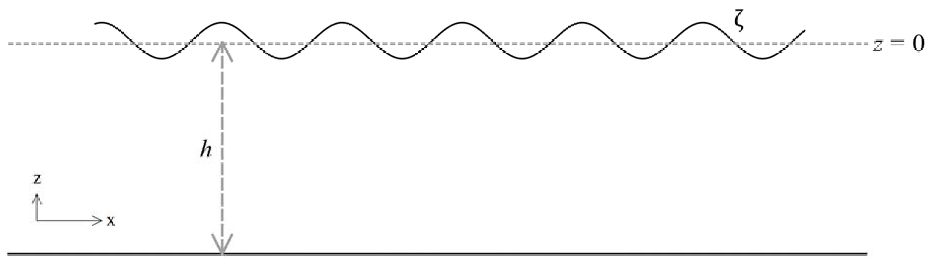
Figure 2.
For glycerin at , the first 10 branches of imaginary parts of frequencies are illustrated. When K increases, the two lowest branches meet and give rise to a nonzero real part, but the majority of frequencies remain totally imaginary.
Figure 2.
For glycerin at , the first 10 branches of imaginary parts of frequencies are illustrated. When K increases, the two lowest branches meet and give rise to a nonzero real part, but the majority of frequencies remain totally imaginary.
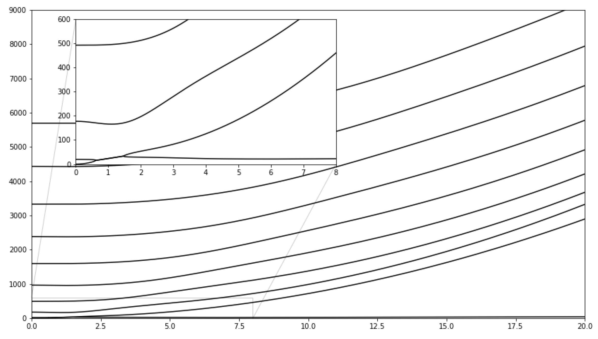
Figure 3.
The real and imaginary parts of frequencies corresponding to the lowest-lying branches versus K for glycerin at ( cm).
Figure 3.
The real and imaginary parts of frequencies corresponding to the lowest-lying branches versus K for glycerin at ( cm).

Figure 4.
The initial wave shape. The defining wave parameters and fluid parameters are water depth: mm; wave height: mm; viscosity: = 0.0011197 ; density: (kg/m³); surface tension: (N/m).
Figure 4.
The initial wave shape. The defining wave parameters and fluid parameters are water depth: mm; wave height: mm; viscosity: = 0.0011197 ; density: (kg/m³); surface tension: (N/m).
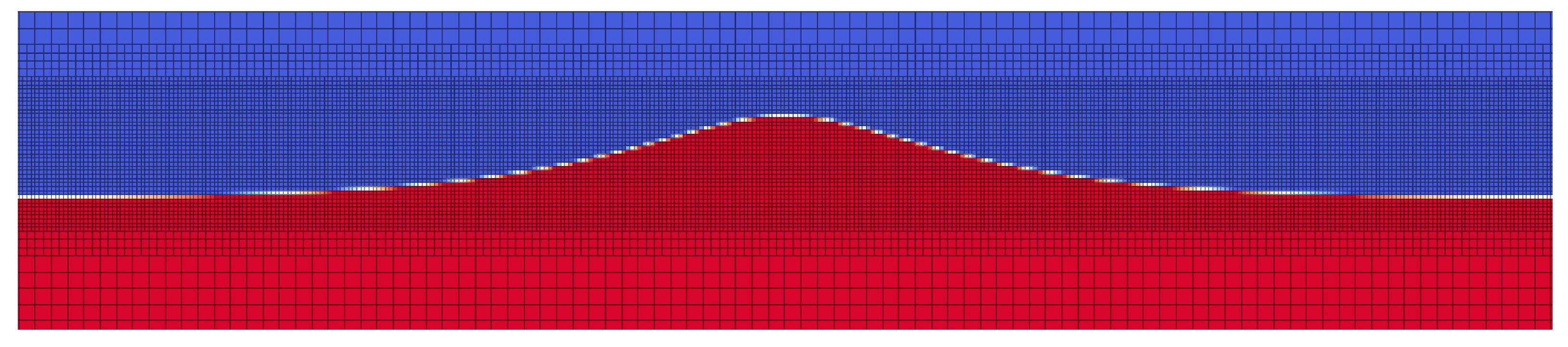
Figure 5.
Comparing theoretical (b) and direct simulation (a) results.

Table 1.
Comparing literature studies by physical parameters.
| Authors | Finite Depth | Viscosity | Surface Tension | Exact Dispersion Relation | Method |
|---|---|---|---|---|---|
| Harrison [15] | X | ✓ | ✓ | X | Perturbation expansion |
| Dias and Kharif [16] | X | X | X | ✓ | – |
| Hunt [17] | ✓ | X | X | X | Levi–Civita’s method |
| Tsuji and Nagata [18] | X | X | ✓ | X | Perturbation expansion |
| Matsuno [1] | ✓ | X | X | X | Principles of complex functions and a methodical perturbation theory |
| Dysthe [22] | X | X | X | X | Perturbation expansion |
| Dias, Dyachenko and Zakharov [26] | X | ✓ | X | X | Helmholtz decomposition |
| Le Meur [34] | ✓ | ✓ | ✓ | ✓ | Boussinesq approximation |
| Armaroli [35] | X | ✓ | ✓ | ✓ | – |
| Ghahraman and Bene [33] | ✓ | ✓ | ✓ | ✓ | Linear approximation |
Disclaimer/Publisher’s Note: The statements, opinions and data contained in all publications are solely those of the individual author(s) and contributor(s) and not of MDPI and/or the editor(s). MDPI and/or the editor(s) disclaim responsibility for any injury to people or property resulting from any ideas, methods, instructions or products referred to in the content. |
© 2023 by the authors. Licensee MDPI, Basel, Switzerland. This article is an open access article distributed under the terms and conditions of the Creative Commons Attribution (CC BY) license (https://creativecommons.org/licenses/by/4.0/).
Share and Cite
MDPI and ACS Style
Ghahraman, A.; Bene, G. Comprehensive Perturbation Approach to Nonlinear Viscous Gravity–Capillary Surface Waves at Arbitrary Wavelengths in Finite Depth. Fluids 2023, 8, 218. https://doi.org/10.3390/fluids8080218
AMA Style
Ghahraman A, Bene G. Comprehensive Perturbation Approach to Nonlinear Viscous Gravity–Capillary Surface Waves at Arbitrary Wavelengths in Finite Depth. Fluids. 2023; 8(8):218. https://doi.org/10.3390/fluids8080218
Chicago/Turabian StyleGhahraman, Arash, and Gyula Bene. 2023. "Comprehensive Perturbation Approach to Nonlinear Viscous Gravity–Capillary Surface Waves at Arbitrary Wavelengths in Finite Depth" Fluids 8, no. 8: 218. https://doi.org/10.3390/fluids8080218