

A Meshless Algorithm for Modeling the Gas-Dynamic Interaction between High-Inertia Particles and a Shock Layer
Moscow Aviation Institute, National Research University, Volokolamskoye sh. 4, 125993 Moscow, Russia
*
Author to whom correspondence should be addressed.
Fluids 2023, 8(2), 53; https://doi.org/10.3390/fluids8020053
Submission received: 31 December 2022
/
Revised: 26 January 2023
/
Accepted: 30 January 2023
/
Published: 2 February 2023
(This article belongs to the Special Issue Focus on Supercritical Fluids: Control and Extraction)
Abstract
:This paper is devoted to numerical modeling of a supersonic flow around a blunt body by a viscous gas with an admixture of relatively large high-inertia particles that, after reflection from the surface, may go beyond the shock layer and change the flow structure dramatically. To calculate the gas-dynamic interaction of moving particles with the shock layer, it is important to take into account the large difference in scales of the flow around the particles and around the body. To make the computations effective, we use a meshless method to solve non-stationary Navier–Stokes equations. The algorithm is based on the approximation of partial derivatives by the least squares method on a set of nodes distributed in the calculation area. Each moving particle is surrounded by a cloud of calculation nodes belonging to its domain and moving with it in space. The algorithm has been tested on the problem of the motion of a single particle and a pair of particles in a supersonic flow around a sphere.
1. Introduction
A dispersed admixture in a supersonic flow may have a multifactorial effect on a streamlined body: direct impacts with the surface, contributing to energy transfer from particles to the body surface and erosive destruction [1], the reverse effect of particles on the gas flow [2,3] and convective heat flux enhancement [4,5], and radiative heat transfer between particles and the body surface [6]. A detailed review of publications on dusty flows around bodies is given in [7,8].
One of the important problems connected with supersonic heterogeneous flows is the gas dynamical interaction of high-inertia particles and a shock layer. By high-inertia particle, we mean relatively large particles that, having reflected from the body surface, can overcome the shock layer and go beyond the bow shock. As experiments have shown [9,10,11], when moving towards a supersonic oncoming flow, such particles can significantly rearrange the flow pattern, change the form and position of the bow shock, and contribute to a multiple increase in the convective heat flux to the body surface. In our previous work, we studied this process numerically. A detailed description of the resulting wave and vortex patterns is given in the papers [12,13,14].
It should be noted that the process of gas-dynamic interaction of particles with a shock layer is extremely difficult for numerical simulation. This is due to the mobility of particles and a significant difference in scales—the linear dimensions of the streamlined body and even relatively large particles differ by several orders of magnitude. In [12,13,14], we used the finite volume method on adaptive Cartesian grids. It allowed us to perform numerical simulation in both the axisymmetric and planar two-dimensional formulations. However, the use of Cartesian grids and the need for a detailed resolution of the boundary layer make it difficult to carry out three-dimensional calculations due to the very large number of computational cells.
There are several effective numerical approaches for solving gas dynamic problems with moving objects. Chimera-type overlapping grid technology [15,16], which uses finite volume or finite difference methods, is based on combining several high-resolution grids related to each of the moving objects and adapted them to their geometry into a single computational grid. The implementations of this approach on structured and unstructured grids are known [17,18]. Another approach involves the use of sliding grids [19,20,21]. It is based on the interpolation of gas flow parameters obtained by calculation on one grid in order to transfer them to another grid, moving relative to the first one, in overlapping areas. This approach has been applied for modeling rotating turbine blades, helicopter propellers, and solving other problems with known trajectories of moving objects [22,23]. In [14], we used sliding grids to calculate the single particle interaction with the shock layer. A serious problem with the considered approaches is the complexity of modeling the interaction between the objects. We face such situations when reproducing collisions between particles or their reflections from the surface.
Therefore, when constructing a three-dimensional computational model, a significantly different approach was chosen, which is based on a meshless method for solving a system of gas dynamics equations [24]. Unlike the finite volume method, which divides the entire calculation area into closed cells, the meshless method uses a finite set of points—calculation nodes. Nodes can be distributed in space in an anisotropic manner, which significantly saves computational resources [24]. Two methods for approximating derivatives have become widespread: based on radial basis functions [25,26,27] and the least squares method [28,29,30]. The latest one is used in this article. This method, despite its relative simplicity, showed a satisfactory agreement between the calculation results and the reference data when solving model problems of supersonic viscous and inviscid flows around a body.
In Section 2, we give a detailed description of the meshless algorithm. To calculate the gas-dynamic interaction of particles with the shock layer, it is important to take into account the large difference in scales of flow around the particles and around the body. For this purpose, we propose the following approach: Along with the stationary main set of nodes, each moving particle is surrounded by its own local cloud of points belonging to its domain. Clouds of computing nodes moving in space together with particles interact with each other, forming a single connected cloud of nodes. When calculating the fluxes, the nodes’ belonging to different domains and their relative velocities are taken into account. The algorithm verification is carried out. The results of calculating the motion of a particle in a gas at rest and the free flow around a stationary particle at the same relative velocity turned out to be identical. In Section 3. we present the results of the numerical simulation of the motion of a single particle and a pair of particles in a supersonic flow around a sphere.
2. Materials and Methods
Governing equations
The model of the viscous heat-conducting gas flow in three-dimensional space includes a system of non-stationary Navier–Stokes equations in combination with the equation of state for ideal gas:
where is the time, is the density, is the pressure, is the temperature, , , and are the components of the gas velocity vector along the coordinate axes , , and , , is the heat capacity ratio is the total gas , and are the inviscid flux , and are the viscous flux vectors along the coordinate axes.
Components of the viscous stress tensor are:
The heat flux density is determined by a vector with components:
The value of dynamic viscosity is calculated using the well-known Sutherland formula:
, , for air.
The thermal conductivity coefficient is proportional to the dynamic viscosity:
where Cp is the specific heat capacity of the gas at constant pressure and Pr is the Prandtl number.
At the entrance to the computational domain, the Dirichlet boundary conditions are set, which determine the incoming supersonic flow with a fixed temperature , pressure, and velocity. At the output—the Neumann conditions are set, where is the outer normal to the boundary.
The body surface is considered isothermal with a known temperature . No-slip and impermeability conditions are set here, as well as the condition .
Meshless Method
To represent the field of gas-dynamic quantities in the computational domain, a finite set of discrete points with a fixed location in space is formed. Near the body surface, the points cluster in the normal direction in order to resolve the flow in the boundary layer in detail (see Figure 1).
The least square method serves as the basis for approximating a scalar function while having the values in a discrete set of points. For each computational node and the cloud of neighboring nodes surrounding it (see Figure 2), approximate equalities are written:
According to the least square method, the optimal approximation of the partial derivatives , , is achieved by minimizing the functional
where the weight coefficients are inversely proportional to the distance between a node and its neighbors:
The values of the linear combination coefficients can be obtained by solving a system of linear equations:
In the numerical solution of the system of gas dynamics equations, the components of the velocity vector, pressure, temperature, gas density, and complex functions containing them, as well as components of viscous and convective fluxes, act as function . The system of Navier–Stokes equations in a semi-discrete form takes the form:
The calculation of the convective flux vectors , , in the middle of the segment connecting the nodes and , according to the AUSMPW+ scheme [31], requires two passes over the set of points. At the first stage, the vectors of conservative variables , are reconstructed by applying the MUSCL scheme with the van Albada 2 limiter to the vector of primary variables [32]:
where the coefficient determines the approximation order of the reconstruction scheme, at the third order is realized, and at or the second order takes place. In this work, we use , .
For each pair of nodes, and , the minimum pressure value and the coefficient at all interfaces between the nodes and and their immediate neighbors are calculated. Here and are the pressure values for and , respectively.
At the second stage, using the values and , and the state vectors and for a pair of nodes and , the calculation of the convective fluxes vectors is performed. To generalize the presented method, we introduce the vectors and , depending on the flux vector direction:
Then the normal projection of the velocity is . The procedure for calculating the convective flux vector along the axis is described in detail below. In this case, . Algorithms for calculating vectors , are similar to the one given below, taking into account the vector and velocity projections ( и ).
Depending on the direction of the vector, , , and are selected:
The enthalpy, speed of sound, and Mach numbers are calculated:
where is the total enthalpy and is the tangential velocity component.
Coefficients are calculated as follows:
The expression for calculating the convective flux has the form
Partial spatial derivatives of temperature and velocity components are required to calculate the elements of the viscous stress tensor and the heat flux vector:
The obtained values are directly used to calculate the viscous flux vectors , , in the node according to the above expressions.
The reconstruction of the gradient vectors of physical variables , , , is required to calculate the viscous fluxes , , in the middle of the segment, connecting the nodes and . It is performed according to [28]:
Let us give some expressions:
The remaining components of the viscous stress tensor are calculated in a similar way.
Numerical integration with respect to time is performed by the third-order explicit Runge–Kutta method [32]:
The time step for explicit integration is determined according to the Courant criterion:
by Roe-averaging vectors of physical variables for and
The implementation of the Neumann boundary conditions is also based on the approximation of the derivative by the least squares method [28]:
where , , are the components of the outward normal vector at node on the surface boundary and is the set of its neighboring nodes that do not belong to the boundary (see Figure 3).
The calculation of the components of the gas state vector at node at the isothermal wall with temperature is carried out according to the expressions:
Modeling the motion of particles in a gas flow
The developed computational model makes it possible to study the supersonic flow of a viscous gas in the presence of one or several relatively large moving particles. The flow around each object (the body and the particles) is calculated by solving the system of gas dynamics equations in its own coordinate system on a selected set of calculation nodes belonging to its domain. A body in a supersonic flow is considered immovable along with its coordinate system, the domain, and the cloud of nodes, which are further referred to as the “main”. On the inlet boundary of the main computational domain, the parameters of the oncoming flow are set (—the normal vector to the boundary):
The Neumann boundary conditions are set at the exit from the main calculation area:
The aerodynamic drag force, , which determines the change in particle velocity, is calculated from the action of the viscous friction force and the gas pressure at the computational nodes on its surface:
where is the particle mass, is the particle velocity vector, and is the particle position vector in the central coordinate system. The boundary nodes lying on the particle surface correspond to the surface elements with area , and the outer normal vector , is the tangential component of the gas velocity near the surface.
In the computational domain, a stationary set of computing nodes belonging to the main domain, adapted to the boundaries of the domain and the geometry of the object, is formed. Each particle is surrounded by a cloud of computational nodes that belong to its domain and move with it in space. The solution of the gas dynamics equations at the nodes connected with the particle is carried out in the local moving coordinate system, whereas at the nodes of the main domain—it is in the central fixed coordinate system. As the particle moves in space, some of the computational nodes are temporarily excluded from the calculation, and the outer boundary nodes of the particle domain become neighbors with the nodes of the main domain or the domain of another particle (see Figure 4). When numerically integrating the equations using a meshless method, the calculation of viscous and convective fluxes between nodes belonging to different domains requires the transformation of the conservative variables’ vectors, , as well as their gradients, , into the local coordinate system of the node for which the calculation is performed.
An approach based on the use of a single cloud of computational nodes makes it possible to simulate the gas-dynamic interaction of a particle with the body as well as the interaction between the particles.
The software implementation of the described algorithms is made in the C++ programming language in combination with the OpenCL parallel computing technology, which allows the use of heterogeneous parallel computing devices, including graphics processors from different manufacturers.
A series of computational experiments have been carried out to test the operation of the presented method for simulating gas flow around moving objects. In one of the series of tests, the flow around a sphere was calculated in the following modes:
- the sphere is at rest , the Mach number of the oncoming flow ;
- the sphere moves against the oncoming flow (), the sphere velocity corresponds to Mach number
- the gas is stationary , the sphere moves with the velocity corresponding to Mach number
3. Results and Discussion
A computational experiment was carried out to simulate the motion of a large spherical particle with a diameter of silicon dioxide and a density along the symmetry axis of a sphere with a diameter toward the oncoming flow. The Mach and Reynolds numbers of the oncoming flow are and . The initial velocity of the particle starting from the sphere surface is . Figure 7 shows the shadow patterns of the flow at successive times , , , , , , and in Figure 8, the distributions of the pressure and convective heat flux along the surface are presented that correspond to those time moments. The angular coordinate here is counted from the critical point. The value of the heat flux is normalized by the value of the heat flux at the critical point, calculated with the well-known Fay–Riddell formula [33].
When the particle passes through the head shock wave, the stationary shock-wave structure is destroyed, resulting in the formation of a cone-shaped perturbation region, the top of which is moving along with the particle. In the zone of contact between the cone-shaped and bow shock waves, a -configuration of three waves arises with the formation of an impact jet directed towards the surface, which causes a significant increase in pressure and in the heat flux in the local area affected by the jet (see Figure 8). As the particle moves away from the surface, the wave configuration evolves, and the zone of their contact, together with the region of the intense gas impact on the surface, shifts to the periphery. A detailed analysis of the observed phenomena and mechanisms of their occurrence is given in [12], where a similar problem is solved by the finite volume method on adaptive Cartesian grids.
Figure 9 shows the shadow patterns of the flow when two identical particles are sequentially launched at an angle to the symmetry axis. In the considered configuration, the second particle finds itself under the influence of the wake of the first particle, loses the velocity component faster, and, as a result, moves away from the sphere to a noticeably smaller distance before turning around and moving to the periphery.
Figure 10 shows graphs of the pressure and the convective heat flux along the surface at the time instants corresponding to the flow patterns in Figure 9. There is an approximately two times increase in the pressure and an almost four times increase in the heat flux in a local area near the critical point. Significant perturbations of the gas parameters near the surface, leading to the appearance of regions of multiple enhancement of the convective heat flux, accompany the particles during their movement.
4. Conclusions
A meshless algorithm has been proposed for modeling the gas-dynamic interaction of moving particles with the shock layer. The algorithm allows for overcoming the problems connected with the large difference in scales of the flow around the particles and around the body. The algorithm is based on the approximation of partial derivatives by the least squares method on a set of nodes distributed in the calculation area. Along with the stationary main set of nodes, each moving particle is surrounded by its own cloud of points belonging to its domain. Clouds of computational nodes moving in space together with particles interact with each other, forming a single connected cloud of nodes. When calculating the fluxes, the nodes’ belonging to different domains and their relative velocities are taken into account. Numerical experiments have been carried out to simulate the motion of a single particle and a pair of particles in a supersonic flow around a sphere. The developed algorithm opens up wide opportunities for the detailed study of the collective effects of a coarsely dispersed admixture on the flow and heat transfer in the shock layer for a blunt body in a supersonic flow.
Author Contributions
Methodology, software, and investigation, A.S.; methodology, investigation, and validation, D.R. All authors have read and agreed to the published version of the manuscript.
Funding
This research was carried out within the framework of the state assignment issued by the Ministry of Education and Science of Russia under project number FSFF-2020-0013.
Institutional Review Board Statement
Not applicable.
Informed Consent Statement
Not applicable.
Data Availability Statement
Not applicable.
Conflicts of Interest
The authors declare no conflict of interest.
References
- Ershova, T.V.; Mikhatulin, D.S.; Reviznikov, D.L.; Sposobin, A.V.; Vinnikov, V.V. Numerical Simulation of Heat and Mass Transfer between Heterogeneous Flow and an Obstacle. Comput. Therm. Sci. 2011, 3, 15–30. [Google Scholar] [CrossRef]
- Tsirkunov, Y.M. Gas-particle flows around bodies—Key problems, modeling and numerical analysis. In Proceedings of the Fourth International Conference on Multiphase Flow—CD ROM Proc. ICMF’2001, New Orleans, LA, USA, 27 May–1 June 2001; Michaelides, E., Ed.; Paper No. 609. [Google Scholar]
- Molleson, G.V.; Stasenko, A.L. Acceleration of Microparticles and their Interaction with a Solid Body. High Temp. 2017, 55, 906–913. [Google Scholar] [CrossRef]
- Oesterlé, B.; Volkov, A.N.; Tsirkunov, Y.M. Numerical investigation of two-phase flow structure and heat transfer in a supersonic dusty gas flow over a blunt body. Prog. Flight Phys. 2013, 5, 441–456. [Google Scholar]
- Osiptsov, A.N.; Egorova, L.A.; Sakharov, V.I.; Wang, B. Heat transfer in supersonic dusty-gas flow past a blunt body with inertial particle deposition effect. Prog. Nat. Sci. 2002, 12, 887–892. [Google Scholar]
- Reviznikov, D.L.; Sposobin, A.V.; Dombrovsky, L.A. Radiative Heat Transfer from Supersonic Flow with Suspended Polydisperse Particles to a Blunt Body: Effect of Collisions between Particles. Comput. Therm. Sci. 2015, 5, 313–325. [Google Scholar] [CrossRef]
- Varaksin, A.Y. Fluid dynamics and thermal physics of two-phase flows: Problems and achievements. High Temp. 2013, 51, 377–407. [Google Scholar] [CrossRef]
- Varaksin, A.Y. Gas-Solid Flows Past Bodies. High Temp. 2018, 56, 275–295. [Google Scholar] [CrossRef]
- Fleener, W.A.; Watson, R.H. Convective heating in dust-laden hypersonic flows. In Proceedings of the 8th Thermophysics Conference, Palm Springs, CA, USA, 16–18 July 1973. AIAA Paper 1973, No. 73-761. [Google Scholar]
- Holden, M.S.; Duryea, G.; Gustafson, G.; Hudack, L. An Experimental Study of Particle-Induced Convective Heating Augmentation. In Proceedings of the 9th Fluid and Plasma Dynamics Conference, San Diego, CA, USA, 14–16 July 1976. AIAA Paper 1976, No. 76-320. [Google Scholar]
- Vladimirov, A.S.; Ershov, I.V.; Makarevich, G.A.; Khodtsev, A.V. Experimental investigation of the process of interaction between heterogeneous flows and flying bodies. High Temp. 2008, 46, 512–517. [Google Scholar] [CrossRef]
- Reviznikov, D.L.; Sposobin, A.V.; Ivanov, I.E. Change in the Structure of a Flow under the Action of Highly Inertial Particle when a Hypersonic Heterogeneous Flow Passes over a Body. High Temp. 2018, 56, 884–889. [Google Scholar] [CrossRef]
- Reviznikov, D.L.; Sposobin, A.V.; Ivanov, I.E. Comparative Analysis of Calculated and Experimental Data on an Oscillating Flow Induced by the Gasdynamic Interaction of a Particle with a Shock Layer. High Temp. 2020, 58, 839–845. [Google Scholar] [CrossRef]
- Sposobin, A.V.; Reviznikov, D.L. Impact of High Inertia Particles on the Shock Layer and Heat Transfer in a Heterogeneous Supersonic Flow around a Blunt Body. Fluids 2021, 6, 406. [Google Scholar] [CrossRef]
- Benek, J.A.; Buning, P.G.; Steger, J.L. A 3-D Chimera Grid Embedding Technique. In Proceedings of the 7th Computational Physics Conference, Cincinnati, OH, USA, 15–17 July 1985. AIAA Paper 1985, No. 85-1523. [Google Scholar]
- Wang, Z.J.; Parthasarathy, V. A Fully Automated Chimera Methodology for Multiple Moving Body Problems. Int. J. Numer. Methods Fluids 2000, 33, 919–938. [Google Scholar] [CrossRef]
- Lee, K.R.; Park, J.H.; Kim, K.H. High-Order Interpolation Method for Overset Grid Based on Finite Volume Method. AIAA J. 2011, 49, 1387–1398. [Google Scholar] [CrossRef]
- Deryugin, Y.N.; Sarazov, A.S.; Zhuchkov, R.N. Features of overset meshes methodology on unstructed grids. Math. Model. Comput. Simul. 2017, 9, 587–597. [Google Scholar] [CrossRef]
- Bakhvalov, P.A.; Bobkov, V.G.; Kozubskaya, T.K. Application of schemes with a quasi-one-dimensional reconstruction of variables for calculations on nonstructured sliding grids. Math Model. Comput Simul. 2017, 9, 155–168. [Google Scholar] [CrossRef]
- Yamakawa, M.; Chikaguchi, S.; Asao, S.; Hamato, S. Multi Axes Sliding Mesh Approach for Compressible Viscous Flows. In Computational Science—ICCS 2020; Krzhizhanovskaya, V., Závodszky, G., Lees, M.H., Dongarra, J.J., Sloot, P.M.A., Brissos, S., Teixeira, J., Eds.; Lecture Notes in Computer Science; Springer: Cham, Switzerland, 2020; Volume 12143, pp. 46–59. [Google Scholar]
- Dürrwächter, J.; Kurz, M.; Kopper, P.; Kempf, D.; Munz, C.; Beck, A. An efficient sliding mesh interface method for high-order discontinuous Galerkin schemes. Comput. Fluids 2021, 217, 104825. [Google Scholar] [CrossRef]
- Steijl, R.; Barakos, G. Computational Investigation of Rotor–Fuselage Interactional Aerodynamics using Sliding–Plane CFD Method. AIAA J. 2009, 47, 2143–2157. [Google Scholar] [CrossRef]
- Nam, H.J.; Park, Y.; Kwon, O.J. Simulation of Unsteady Rotor–Fuselage Aerodynamic Interaction Using Unstructured Adaptive Meshes. J. Am. Helicopter Soc. 2006, 51, 141–149. [Google Scholar] [CrossRef]
- Li, H.; Mulay, S.S. Meshless Methods and Their Numerical Properties; CRC Press: New York, NY, USA, 2013. [Google Scholar]
- Vasilyev, A.N.; Kolbin, I.S.; Reviznikov, D.L. Meshfree computational algorithms based on normalized radial basis functions. In Advances in Neural Networks; Cheng, L., Liu, Q., Ronzhin, A., Eds.; Notes in Computer Science; Springer: Cham, Switzerland, 2016; Volume 9719, pp. 583–591. [Google Scholar]
- Li, J.; Hon, Y. Domain Decomposition for Radial Basis Meshless Methods. Numer. Methods Part. Differ. Equ. 2004, 20, 450–462. [Google Scholar] [CrossRef]
- Tolstykh, A.I.; Shirobokov, D.A. Meshless method based on radial basis functions. Comput. Math. Math. Phys. 2005, 45, 1447–1454. [Google Scholar]
- Hashemi, M.Y.; Jahangirian, A. Implicit fully mesh-less method for compressible viscous flow calculations. J. Comput. Appl. Math. 2011, 235, 4687–4700. [Google Scholar] [CrossRef]
- Sattarzadeh, S.; Jahangirian, A. 3D implicit mesh-less method for compressible flow calculations. Sci. Iran. 2012, 19, 503–512. [Google Scholar] [CrossRef]
- Sattarzadeh, S.; Jahangirian, A.; Hashemi, M.Y. Unsteady Compressible Flow Calculations with Least-Square Mesh-less Method. J. Appl. Fluid Mech. 2016, 9, 233–241. [Google Scholar] [CrossRef]
- Kim, K.H.; Kim, C.; Rho, O.H. Methods for the accurate computations of hypersonic flows I. AUSMPW+ Scheme. J. Comput. Phys. 2001, 174, 38–80. [Google Scholar] [CrossRef]
- Wang, Y.; Cai, X.; Zhang, M.; Ma, X.; Ren, D.; Tan, J. The study of the three-Dimensional meshless solver based on AUSM+-up and MUSCL scheme. In Proceedings of the 2015 International Conference on Electromechanical Control Technology and Transportation, Zhuhai, China, 31 October–1 November 2015. [Google Scholar] [CrossRef]
- Fay, J.A.; Riddell, F.R. Theory of stagnation point heat transfer in dissociated air. J. Aeronaut. Sci. 1958, 25, 73–85. [Google Scholar] [CrossRef]
Figure 1.
Location of computing nodes: on the body surface (a), in the section of the computational domain (b).
Figure 1.
Location of computing nodes: on the body surface (a), in the section of the computational domain (b).

Figure 2.
Clouds of computing points surrounding nodes i and j.

Figure 3.
Implementation of the boundary conditions on the body surface.
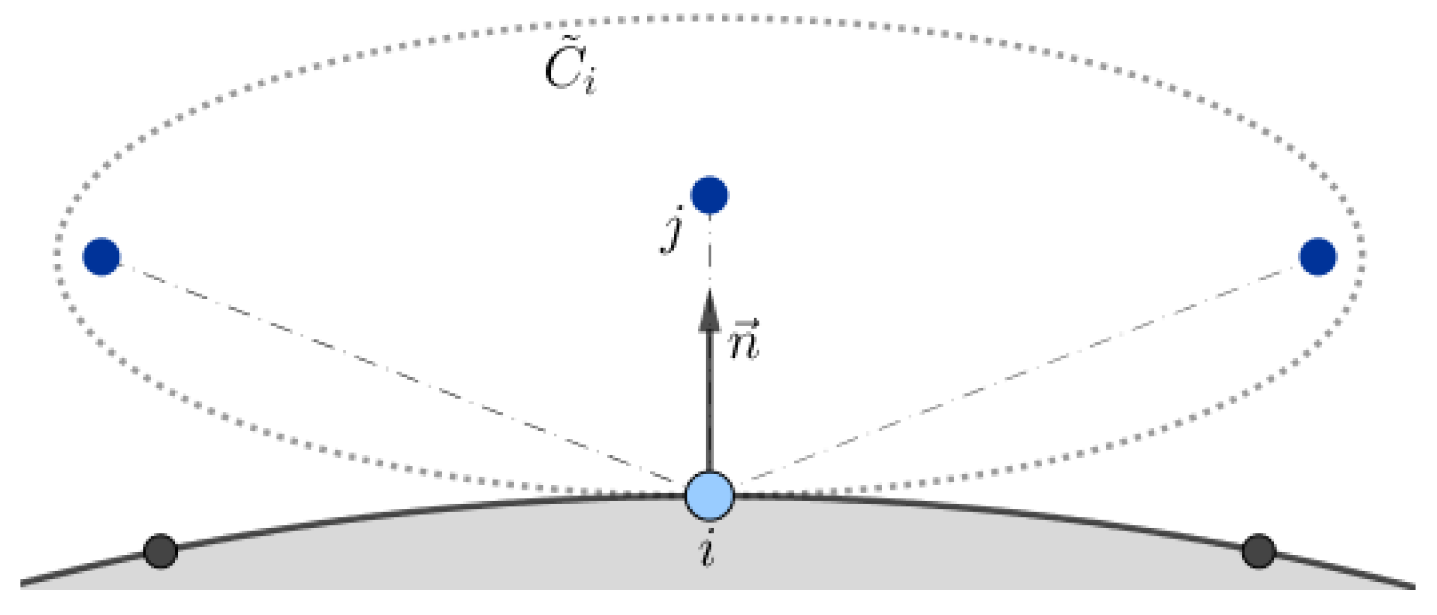
Figure 4.
Formation of a single cloud from nodes belonging to different domains.

Figure 5.
Shadow pattern of the flow around the sphere (single cloud of nodes).
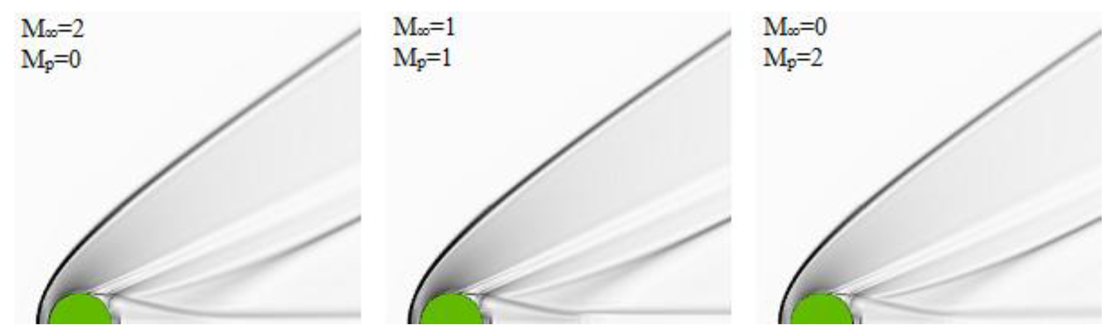
Figure 6.
Distribution of the gas pressure along the sphere surface.
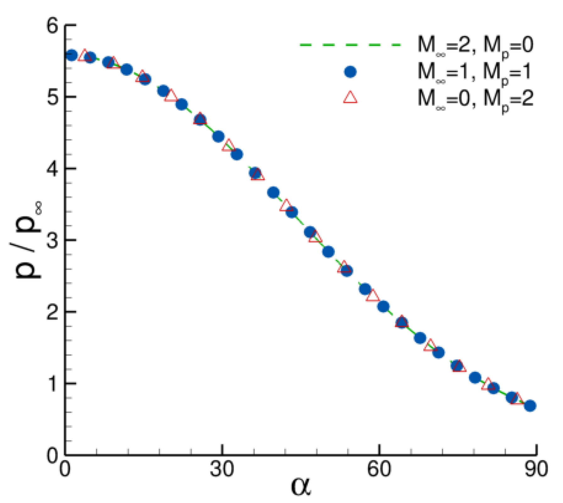
Figure 7.
(a). Shadow pictures of the flow in the process of particle movement along the symmetry axis. (b). Shadow pictures of the flow in the process of particle movement along the symmetry axis (continued).
Figure 7.
(a). Shadow pictures of the flow in the process of particle movement along the symmetry axis. (b). Shadow pictures of the flow in the process of particle movement along the symmetry axis (continued).
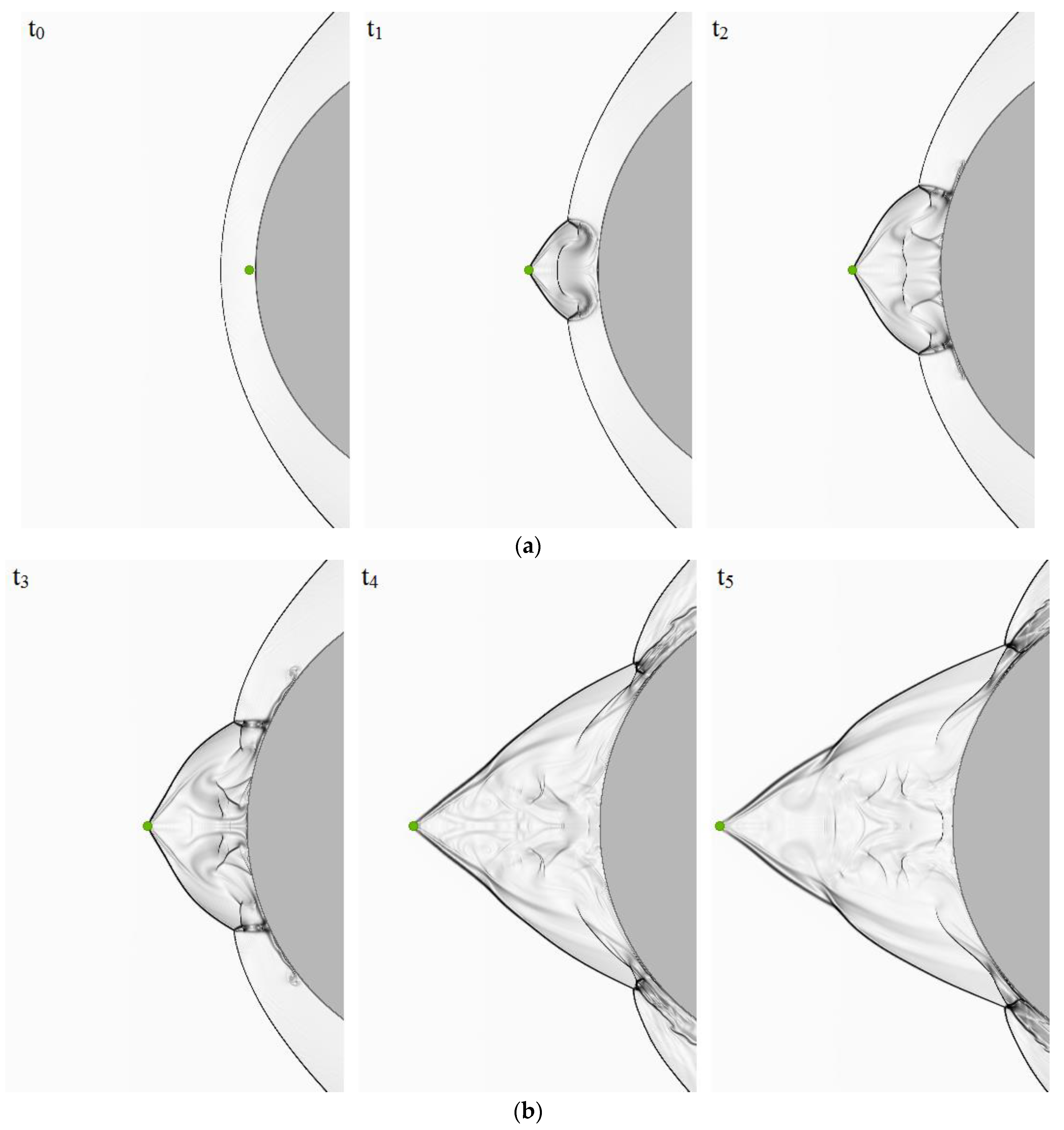
Figure 8.
Oscillations of the pressure (a) and the convective heat flux (b) on the surface, induced by the gas-dynamic interaction of a particle with a shock layer.
Figure 8.
Oscillations of the pressure (a) and the convective heat flux (b) on the surface, induced by the gas-dynamic interaction of a particle with a shock layer.

Figure 9.
Shadow pictures of the flow under the influence of a pair of particles.

Figure 10.
Pressure (a) and convective heat flux (b) oscillations on the sphere surface, induced by the gas-dynamic interaction of a pair of particles with a shock layer.
Figure 10.
Pressure (a) and convective heat flux (b) oscillations on the sphere surface, induced by the gas-dynamic interaction of a pair of particles with a shock layer.

Disclaimer/Publisher’s Note: The statements, opinions and data contained in all publications are solely those of the individual author(s) and contributor(s) and not of MDPI and/or the editor(s). MDPI and/or the editor(s) disclaim responsibility for any injury to people or property resulting from any ideas, methods, instructions or products referred to in the content. |
© 2023 by the authors. Licensee MDPI, Basel, Switzerland. This article is an open access article distributed under the terms and conditions of the Creative Commons Attribution (CC BY) license (https://creativecommons.org/licenses/by/4.0/).
Share and Cite
MDPI and ACS Style
Sposobin, A.; Reviznikov, D. A Meshless Algorithm for Modeling the Gas-Dynamic Interaction between High-Inertia Particles and a Shock Layer. Fluids 2023, 8, 53. https://doi.org/10.3390/fluids8020053
AMA Style
Sposobin A, Reviznikov D. A Meshless Algorithm for Modeling the Gas-Dynamic Interaction between High-Inertia Particles and a Shock Layer. Fluids. 2023; 8(2):53. https://doi.org/10.3390/fluids8020053
Chicago/Turabian StyleSposobin, Andrey, and Dmitry Reviznikov. 2023. "A Meshless Algorithm for Modeling the Gas-Dynamic Interaction between High-Inertia Particles and a Shock Layer" Fluids 8, no. 2: 53. https://doi.org/10.3390/fluids8020053