
POD-Based Model-Order Reduction for Discontinuous Parameters


NAVASTO GmbH, D-10553 Berlin, Germany
Fluids 2022, 7(7), 242; https://doi.org/10.3390/fluids7070242
Submission received: 11 June 2022
/
Revised: 6 July 2022
/
Accepted: 12 July 2022
/
Published: 14 July 2022
(This article belongs to the Special Issue Aerodynamics of Road Vehicles and Trains)
Abstract
:Reduced-order models (ROMs) based on proper orthogonal decomposition (POD) are widely used in industry. Due to the rigid requirements on the input data, these methods struggle with discontinuous parameters, e.g., optional rear spoiler on a car. In order to also include these types of parameters, a new method is presented that splits the full-order model (FOM) domain with its discontinuous parameters into multiple ROM subdomains. The resulting subdomains then again comply with the ROM requirements, and the established and proven ROM methods can be applied. The steps involved in computing a ROM based on the proposed method, by setting up the subdomains, mapping the FOM data into the domains, as well as computing the ROMs on the domains, are shown in detail in this paper. The method is employed on two use cases. The academic one-dimensional use case focuses on how the steps involved are employed and analyzes the introduced errors. The second use case’s FOM is based on the DrivAer body with an optional rear spoiler computed using computational fluid dynamics (CFD) and demonstrates the usage in an industrial environment.
1. Introduction
Reduced-order models (ROMs) nowadays play an important role in industry and significantly improve how full-order model (FOM) results are used with respect to optimization problems, merging experimental and numerical data as well as within an interactive design process [1,2,3]. By computing FOM solution snapshots for various parameter combinations in the so-called offline phase, these results can be evaluated and exploited in near real time during the online phase. In this paper, the order reduction is performed using proper orthogonal decomposition (POD) [4] coupled with a radial basis function (RBF) [5] interpolation method (POD+I) for predictions of unknown parameter combinations. The main FOM input in mind is a computational fluid dynamic (CFD) solution.
Utilizing POD+I, especially for industrial use cases, is often not straight forward, since many aspects of the POD computation needs to be taken into account. Due to the POD requirement of conform meshes across the input snapshots, these methods struggle with:
- Discontinuous parameters.
- Complex geometry transformations.
- Nonlinear effects across the parameter domain
often times not being modeled accurately.
In this paper, a new approach in dealing with the aforementioned shortcomings is introduced. The proposed method is referred to as Overset POD (oPOD) since it shares some similarities with the overset mesh CFD approach in which multiple overlapping meshes are used within the CFD context.
In the oPOD approach, the ROM domain is separated into multiple subdomains. For each subdomain a POD+I model is computed. The individual predictions for an unknown parameter combination are then merged together for the complete ROM domain. By separating the domains, the POD requirements can be fulfilled more easily. However, this introduces difficulties in mapping the FOM data to the subdomains. The difficulties that can arise are possible subdomain elements, that, due to mesh deformation, are no longer part of the FOM domain. Furthermore, in order to address this issue, an enhanced snapshot reconstruction method is proposed that alleviates this problem, so that the well-established ROM methods can be used.
The main focus of oPOD is to broaden the usage of possible parameters by allowing discontinuous parameters and likely complex geometry transformation or modeling nonlinear effects. This is demonstrated on two test cases. The main applications of oPOD in mind are ROM prediction visualizations in the context of an industry-grade interactive design process.
The novel contribution of this paper is the proposed oPOD work flow, which models discontinuous parameter and complex geometry transformations by separating the ROM domain. This is covered in Section 2. Another original contribution is an enhancement of the snapshot reconstruction algorithm which is originally based on [6]. This part is covered in Section 3.3.
This paper is organized as follows: Section 2 introduces the oPOD and explains in detail the problem it addresses. Moreover, an overview of similar methods is given and the new contributions of this paper are outlined. In Section 3, the theoretical background and necessary algorithms are introduced and reviewed, followed by Section 4, in which numerical results for an analytic test case as well as the DrivAer body in a full CFD environment are analyzed. The final Section 5 discusses the obtained results.
2. Overset POD Method
In this section, the oPOD method, its terminology, as well as the steps involved in creating and using an oPOD are described. First, the key problems oPOD addresses are explained in detail and a brief overview of the method is given, followed by an in-depth explanation in the following subsections and a summary. In order to better describe and illustrate potential use cases and the oPOD method itself, a schematic CFD case of a parameterized airfoil with and without a flap is utilized, as displayed in Figure 1.
The use case consists of an airfoil in a flow with velocity U and the continuous parameters: angle of attack and trailing flap at position . The discrete parameter controls whether or not a flap is present in the simulation.
2.1. Problem Definition
A hard requirement for using POD is a congruent ordering of values across all snapshots. For snapshots resulting from CFD simulacvtion, the ordering is determined by the CFD index space which is unique for each generated CFD grid. Hence, utilizing snapshots for different geometries is problematic. Utilizing mesh morphing (see [7]) keeps the CFD element order and deforms the mesh with its geometries to a new configuration. Snapshots resulting from these transformations share the same index space and can be used in a POD context. This strategy works well for a wide range of deformation problems but has its short comings. Large or nonlinear deformations can lead to mesh quality degradation and therefore negatively affect the CFD calculations. The same problem applies to deformations close to a wall or stationary object.
This is schematically depicted in Figure 2 for different parameters . The cells between the stationary airfoil and the morphed flap are significantly stretched and a good resolution of the flow characteristics in this region is impaired.
While the problems with mesh deformations are mostly gradual with increasing magnitude of the deformation, it is not possible to model discontinuous parameters with POD. Figure 1 shows the use case with and without a flap. For both cases, a new grid needs to be generated and the resulting snapshots do not share the same CFD index space.
2.2. General oPOD Overview
In general, oPOD uses a set of CFD snapshots that are all based on a consistent set of parameters. Dependent on the use case, the CFD domain is split into multiple oPOD subdomains (step 1). For each subdomain, a new mesh is generated, which can, depending on the oPOD application, be significantly coarser than a CFD mesh. The CFD snapshots are then mapped onto the created oPOD subdomains (step 2) and a subdomain-specific local POD+I reduced-order model is created (step 3). In order to perform an oPOD prediction (step 4), the relevant POD+I models in the corresponding subdomains are queried and the individual predictions are combined to again fill the complete oPOD domain.
2.3. oPOD Domains (Step 1)
The criteria on how the CFD snapshots are split into the oPOD domains are use-case-specific and one of the most critical steps in the oPOD process. During this step, it is important to keep in mind how an oPOD prediction (step 4) is performed and how the multiple oPOD domains interact with one another.
The primary reason for creating an oPOD subdomain is to handle snapshots that are based on different CFD index spaces. As discussed in Section 2.1, the main reasons this occurs are a CFD input deck where no mesh morphing was applied and each snapshot is based on a unique CFD index space.
The subdomain creation is demonstrated below for the discontinuous parameter for the CFD flow example above.
Discontinuous Parameter
In general, a separate oPOD domain decouples certain regions from one another. It is therefore possible to embed a discontinuous CFD snapshot parameter in a single or multiple overlapping domains.
This is visualized in Figure 3 in which the discontinuous CFD snapshot parameter is used to model a single airfoil or an airfoil with a trailing flap. The oPOD domains created based on the CFD domain ![Fluids 07 00242 i001]() is a background domain
is a background domain ![Fluids 07 00242 i002]() that only contains the airfoil for and for a separate foreground domain
that only contains the airfoil for and for a separate foreground domain ![Fluids 07 00242 i003]() . In Figure 3, the background domain almost shares the same bounds as the CFD domain and only models the flow around as well as the wake of airfoil. The foreground domain models the region around the flap and the trailing wake of it.
. In Figure 3, the background domain almost shares the same bounds as the CFD domain and only models the flow around as well as the wake of airfoil. The foreground domain models the region around the flap and the trailing wake of it.
 is a background domain
  that only contains the airfoil for and for a separate foreground domain
  . In Figure 3, the background domain almost shares the same bounds as the CFD domain and only models the flow around as well as the wake of airfoil. The foreground domain models the region around the flap and the trailing wake of it.
A prediction for a sought parameter now would query the model of the background domain and depending on the value of the foreground model (if ). An interpolation region ![Fluids 07 00242 i004]() can be used on the boundary of the foreground domain to smooth out the predictions of the background and foreground models (more on this is discussed in step 4).
can be used on the boundary of the foreground domain to smooth out the predictions of the background and foreground models (more on this is discussed in step 4).
 can be used on the boundary of the foreground domain to smooth out the predictions of the background and foreground models (more on this is discussed in step 4).
In this example, it is quite obvious that the setup of the domains is very dependent on the use case. Since, depending on , the wake of the flow would have significantly different features, the foreground domains need to extend as far into the background domain as necessary in order to accurately model these features. Moreover, any other parameterization or a larger value range for the parameter would lead to a different setup of the foreground domains.
2.4. Mapping Snapshots from CFD to oPOD Domains (Step 2)
After setting up the oPOD domains resulting in new meshes for each domain in step 1, the CFD snapshots need to be mapped onto these meshes. If any geometric deformation on the CFD snapshot was applied, it needs to be applied to the oPOD domain as well by using, among others, radial basis functions [8,9] or the linear elasticity equations [10]. The resulting elements of the deformed oPOD meshes may end up outside of the CFD domain. By using the method of signed distances [11,12] these elements can be identified and are left out of the mapping process.
With the prepared and aligned oPOD domains to the corresponding CFD snapshots, the modeled variables can be mapped from the CFD snapshots to the oPOD domains. Possible mesh interpolation methods are a consistent interpolation scheme such as the advancing front algorithm [13], an R-tree spatial search algorithm [14] or a conservative interpolation method by local Galerkin projection [15].
Another important feature of the mapping process is that not all CFD snapshots need to be mapped onto all oPOD domains. Visiting the example in Figure 3 again shows that each domain only receives snapshots for the corresponding value of . Hence, this parameter is not part of the domain-specific POD+I model since it is constant for all domain-specific snapshots. Moreover, the parameter is irrelevant for the background domain.
2.5. POD+I Creation in oPOD Domains (Step 3)
Once the oPOD domain-specific snapshots are prepared in steps 1 and 2, the POD+I model of each domain can be computed. In the case that all points/cells/elements of the oPOD subdomain are part of the CFD domain, a POD+I model based on the mapped snapshots can be computed. Otherwise, possibly due to transformations, it is possible that the domain for a number of snapshots lie outside of the corresponding CFD domain. In this case, not all variables of the CFD snapshot could be mapped on the corresponding oPOD snapshot domain. In order to also use these snapshots for the local POD+I models, a snapshot reconstruction algorithm needs to be employed. This reconstruction is discussed in detail in Section 3.3.
The Algorithm 1 summarizes steps 2 and 3. It shows how, based on the CFD snapshots and a domain-specific reference grid G, a local oPOD domain POD+I model can be created. By looping over all available CFD snapshots, the relevant domain-specific snapshots are identified and the corresponding parameter vector is transformed to the local domain-specific parameters (lines 3 to 5). If a geometry transformation is applied, the reference grid G is transformed, resulting in a transformed grid . Otherwise, the reference grid G is used (line 6). After mapping the CFD snapshot on the transformed mesh , the resulting snapshots with the corresponding parameters are stored in separate sets (lines 7 to 9). After the loop finishes, the local POD+I model is computed based on the snapshots and parameters present in the stored sets (line 10).
| Algorithm 1 oPOD domain-specific algorithm for local POD+I model creation. |
Require:
|
2.6. oPOD Prediction (Step 4)
An oPOD prediction for a sought parameter is performed by querying the local POD+I models in only the relevant oPOD domains. Since the parameters used by the local POD+I models differ, it is necessary to filter or possibly transform the oPOD parameters to the parameters used by the local models. Depending on the construction of the oPOD domains, the predictions of various oPOD domains can be smoothed out. This is especially necessary if the domains are not large enough to model domain-specific phenomena and a more visualization-driven application is focused. Here, the signed distances from Section 2.4 can be used to smooth out the predictions of the multiple domains.
With the signed distances , computed at each element of the foreground domain with respect to the edge of the domain or a geometric object, and the interpolation distance r, the interpolation region ( ![Fluids 07 00242 i004]() Figure 3) is defined. By mapping the results of the background domain onto the foreground domain (similar to step 2), the predictions and of the fore and background model, respectively, are now present in each element of the foreground domain. The interpolated prediction is now computed with
Figure 3) is defined. By mapping the results of the background domain onto the foreground domain (similar to step 2), the predictions and of the fore and background model, respectively, are now present in each element of the foreground domain. The interpolated prediction is now computed with
Figure 3) is defined. By mapping the results of the background domain onto the foreground domain (similar to step 2), the predictions and of the fore and background model, respectively, are now present in each element of the foreground domain. The interpolated prediction is now computed with
2.7. Summary
An alternative visualization of Algorithm 1 for the creation of the POD+I models in the separate oPOD subdomains is displayed in Figure 4 as a flow chart.
Based on a set of already created oPOD subdomains, Figure 4a displays how, for a specific subdomain , the CFD snapshots and parameter are mapped, transformed and the resulting snapshots and parameters are used to compute the domain-specific model. The details of the “map and transform CFD snapshots” block are shown in Figure 4b. In a loop over all CFD snapshots, it is checked if a specific CFD snapshot with the parameter is relevant for the current oPOD subdomain . If this is the case, then the parameter and reference grid are transformed and the CFD solution is mapped onto the transformed grid . The resulting snapshot and parameter are stored and used to compute the domain-specific model in Figure 4a.
All resulting subdomain models are stored and used again for an oPOD prediction of a sought-after parameter combination as outlined in Section 2.6.
3. Theory
The aim to use or enhance predictions of reduced-order models is a major focus in the field and “…has seen tremendous development in the past two decades, especially in the broad domain of computational mechanics” [16]. An overview of the latest snapshot-based methods for parameterized partial differential equations are available in [1,16].
Related approaches to oPOD can be found in the literature. Shifted POD [17] “…extends the POD by introducing time-dependent shifts of the snapshot matrix” [17]. With this shift, it is possible to improve the POD predictions considerably by reducing the nonlinear effects across the snapshots. While it is not the key focus of this paper, an oPOD subdomain can be transformed and therefore “shifted” analogous the shifted POD, making use of a similar improvement as a consequence. The Domain-Decomposition POD (DD-POD) [7] utilizes POD in the context of CFD in order to model turbulent flows around parameterized geometries. Here, the ROM subdomain is coupled to CFD through an overlapping region using a Schwarz-type method [18], resulting in a nonlocal CFD boundary condition. This is comparable to oPOD in the sense that oPOD subdomains are also coupled to the surrounding domain.
The remaining section reviews the methods involved in computing a POD+I model with a special focus on snapshot reconstruction, which is needed in oPOD in the case the an oPOD subdomain transformation leads to elements outside the FOM domain.
3.1. Radial Basis Functions/Kriging
Radial basis function (RBF) or Kriging models are suitable to model complex functions. A comprehensive guide can be found in [5,19], and a short overview over the core method and features is given here.
With samples and responses , the model approximation of an unknown sample can be approximate by
with , the basis function and the weights . The weights are determined by solving the linear system of equations , with being the Gram matrix which is defined as , [19] (Section 2.3).
Popular choices for the RBF model basis function are thin plate spine (TPS) with and cubic with , with r being the euclidean distance of the two sample points . A characteristic feature of the model basis functions is that their response decreases or increases monotonically with respect to the distance of the two samples [5].
The Kriging basis function is defined with and introduces a varying exponent , which typically is set to either 1 or 2, and a hyperparameter vector , which can be determined by a maximum likelihood estimation [19] (Section 2.4).
3.2. Proper Orthogonal Decomposition
In the field of fluid dynamics, three established reduced-order model-based proper orthogonal decomposition (POD) approaches exist by either using an interpolation coupled method (POD+I) [6,20,21], a CFD flux residual minimization scheme [22,23] or a Galerkin projection-based framework [24]. A comprehensive introduction can be found in [4,16,24]. A brief review of POD is given below.
For a set of independent parameters and CFD flow solution snapshots , ; the snapshot matrix is defined by
By solving the dimensional snapshot correlation eigenvalue problem
the normalized eigenvectors can be found. By ordering the eigenvalues and corresponding eigenvectors based on , the m POD modes form an orthonormal basis, which is given by
Initial snapshots can be expressed with the newly found basis
and an approximate snapshot at an untried parameter combination can be computed by a coefficient vector analogous to Equation (4) with
The coefficient vector can be obtained by interpolating its components with a RBF or Krigin model at the parameter combination based on the data set . The POD coefficient matrix is then defined with and the POD modes with . A mode reduction of is applied to the POD by stripping the last rows and columns from the POD coefficient and modes matrix, respectively.
3.3. POD+I with Snapshot Reconstruction
Based on a snapshot reconstruction method introduced in [6,25], it is possible to iteratively guess and fill possibly missing elements of the snapshots. For a fixed number of iterations, a POD based on the current snapshot ensemble is computed, and the missing elements are repaired by using the resulting POD modes of the current iteration. In [6], a constant number of modes p is proposed. Setting p too low results in only low-level features being set in the missing elements, while setting p too high does not average out the to-be-detected features sufficiently.
In this paper, an improved method is introduced by determining p separately in each iteration of the snapshot reconstruction with the -Score of the corresponding interpolation model of the POD coefficients. The -Score is a measure for the accuracy of a surrogate model. An -Score of 1 denotes a perfect accuracy in the prediction, while an -Score of 0 denotes a model that constantly predicts the expected value of the responses regardless of the model input. Ref. [26] suggests to reduce the modes of a POD based on the -Score of the POD coefficients surrogate models by reducing the modes of the POD to the point that all coefficient surrogates have an . By using the -Score measure in the snapshot reconstruction procedure, it is possible to include the snapshot features depending on the current state of the snapshot ensemble during this iterative process.
The Algorithm 2 enlists in detail the snapshot reconstruction procedure with the initial setup in lines 1 and 2 where the initial snapshot matrix is constructed by setting the missing values to the mean of the snapshot matrix . In iterations, the reduced POD modes and coefficients are obtained with the -Score reduction and an -Score cut-off set to 0 (lines 4–5). Lines 7–9 apply the mask matrix to the modes and a best guess for the POD coefficient vector is computed and applied to the corresponding column of the snapshot matrix of the next iteration (line 10). At last, the final POD modes and coefficients are computed after the loop finishes based on the final snapshot matrix resulting from the last iteration.
| Algorithm 2 Masked POD computation. |
Require:
|
4. Results
In this paper, oPOD is applied on two test cases. Both test cases have a discrete parameter that allows to optionally add or remove a feature to the overall process, splitting the domain into a separate background and a foreground POD+I. The first test case is a two-parameter one-dimensional process of an analytic function. It is well-suited to demonstrate the investigated oPOD method and analyze the effects each step has on the model prediction as well as the introduced errors. The second test case is the DrivAer body [27] with four parameters computed in a CFD environment.
4.1. Analytic Test Case
The analytic test case is split into two subsections. Both sections model the same process y in the domain . The first section analyzes the performance of oPOD when all snapshot data is available to the model, while in the second section, only a subset of the information for the foreground model is available. Here, the reconstruction of the snapshot matrix, as depicted in Section 3.3, is applied. The to-be-modeled process consists of three distinct parameters. With a discrete parameter , and two continuous parameters and , the analytic test case is described by
with the Gaussian function and the parameters and in the parameter space for and . Both the background as well as the foreground model are sampled using an equidistant full-factorial sampling. The snapshots for the background model are obtained by setting and the foreground snapshots by with and leading to 15 samples for the foreground and three samples for the background model. For the oPOD predictions, a signed distance of is used to linearly smooth out the predictions of the foreground and background models.
4.1.1. Full Model Data
As displayed in Figure 5b, the parameter introduces a scaling factor to the Gaussian function, while the parameter shifts a local bell curve which can be seen in Figure 5a. While the background model spans the complete domain, the foreground domain is limited to . Moreover, the foreground model is dynamically shifted according to parameter .
Figure 8 shows how a prediction with oPOD compares with a standard POD+I model. The POD+I model was trained solely on the snapshots with for the complete domain x. As it can be seen in Figure 8a, the strong nonlinearities in the snapshots are difficult to model for the POD+I model. It specifically struggles in the region of the peak of the bell curve. oPOD is better capable of modeling this region, since the foreground domain is shifted along with the curve, and therefore differences in the snapshots are smaller and easier to model (analogous to [17]). Figure 8b shows how the interpolation in oPOD for the background POD+I and the foreground POD+I model is performed. With an interpolation distance set to from the domain boundary, the output of both models is linearly smoothed out. At the domain boundary for , oPOD uses the values of the background model POD+I, while at the values of the foreground model POD+I are used. In between, the values are linearly interpolated with respect to the distance from the domain boundary. This interpolation scheme results in a good approximation to the to-be-modeled process.
The prediction errors across the parameter space for are depicted in Figure 6. The error e is given for parameter and by the model prediction compared with the process true value for varying with . Figure 6a shows the error for the standard POD+I model while Figure 6b shows the errors for the oPOD predictions. It is important to note the different color ranges in the color bars of the two figures. As expected, the errors close to the snapshot sample locations in the parameter space are small and increase with greater distance, but the errors for oPOD compared with POD+I are significantly smaller.
4.1.2. Incomplete Model Data
In contrast to the previous section, only the foreground model is now computed on the bases of incomplete model data. Setting the cut-off length , all data for and is stripped from the snapshot matrix and reconstructed using Algorithm 2. As depicted in Figure 7 with the ![Fluids 07 00242 i005]() areas, the loss in data is for some snapshots in the foreground model significant and reduces the available data to half compared with the full data.
areas, the loss in data is for some snapshots in the foreground model significant and reduces the available data to half compared with the full data.
 areas, the loss in data is for some snapshots in the foreground model significant and reduces the available data to half compared with the full data.
The error introduced with the snapshot reconstruction for the chosen is negligible as the oPOD prediction with missing data almost matches the oPOD without missing data (see Figure 8).
Figure 8b depicts how the foreground and background models are interpolated in the interpolation region. In the range from , the model output is linearly interpolated starting from the output of the background model at and ending at the output of the foreground model at , matching the output of the to-be-modeled process.
The error comparison of oPOD with and without snapshot reconstruction in Figure 9 shows that the error increases due to the reconstruction of the snapshots. Compared with the errors for oPOD without snapshot reconstruction, the largest errors are no longer in between the snapshot samples but on the border of the parameter domain at . This is due to the fact that in those regions errors due to the reconstruction of the snapshots are introduced.
Figure 10 displays how the error introduced in the snapshot reconstruction increases with increasing and the number of missing values in the snapshots data. The plotted cut-off error is the maximum oPOD prediction error for a specific cut-off length
with being the error evaluation for an oPOD with the corresponding . For this academic use case, the error for , in which up to of data is reconstructed, remains very small. For larger , the error increases up to the point where the reconstruction of snapshot data is infeasible, since the portion of data that needs to be reconstructed is too large ( for .
4.2. DrivAer Test Case
The DrivAer body [27] is used to demonstrate the oPOD capabilities for industrial CFD simulations. All snapshots are computed using OpenFOAM [28] with the Reynolds-averaged Navier-Stokes (RANS) equations, a SST turbulence model and a free stream velocity of . Each simulation consists of approximately 50 million cells with the geometries being deformed using mesh morphing based on radial basis functions. The simulation is based on five parameters. The four continuous parameters (see Figure 11) are the diffusor angle at the lower rear body and the position and rotation of the spoiler.
The fifth parameter is discontinuous and controls whether or not the spoiler is part of the CFD domain resulting in a hypercube parameter domain . The to-be-modeled variables are the windowed average velocity field U and pressure coefficient of the last 2000 iterations of the RANS simulations.
Figure 12a shows the oPOD domain decomposition used for the test case. Within the CFD domain ![Fluids 07 00242 i001]() (not displayed in its correct size for visualization purposes), the background domain
(not displayed in its correct size for visualization purposes), the background domain ![Fluids 07 00242 i002]() encapsulates the complete DrivAer body as well as its wake and is responsible for modeling the front of the body, and in case of , also the wake. For , the foreground domain
encapsulates the complete DrivAer body as well as its wake and is responsible for modeling the front of the body, and in case of , also the wake. For , the foreground domain ![Fluids 07 00242 i003]() models the wake and the flow around at the rear of the body. It contains all deformation-affected geometry parts and expands upstream as far as necessary in order to model the upstream effects of the spoiler. Moreover, it extends to the back of the ROM domain due to the dominant effect the spoiler has on the wake of the flow field.
models the wake and the flow around at the rear of the body. It contains all deformation-affected geometry parts and expands upstream as far as necessary in order to model the upstream effects of the spoiler. Moreover, it extends to the back of the ROM domain due to the dominant effect the spoiler has on the wake of the flow field.
(not displayed in its correct size for visualization purposes), the background domain encapsulates the complete DrivAer body as well as its wake and is responsible for modeling the front of the body, and in case of , also the wake. For , the foreground domain models the wake and the flow around at the rear of the body. It contains all deformation-affected geometry parts and expands upstream as far as necessary in order to model the upstream effects of the spoiler. Moreover, it extends to the back of the ROM domain due to the dominant effect the spoiler has on the wake of the flow field.For the results presented below, the foreground domain is modeled using 74 snapshots which are placed in the parameter space using the quasi-random number Halton sequence [29]. The background domain is modeled using five equidistantly distributed samples in the parameter space . While the background model only depends on as its parameter, the foreground model is built using all continuous parameters.
In Figure 12b, the midslice of the applied signed distance field ratio (step 4, Section 2.6) is shown. Setting the interpolation region radius to , all domain boundaries except the rear boundary are interpolated according to Equation (1). The signed distance field is not affected by the DrivAer body since the foreground model should be used directly in the wake.
4.2.1. oPOD Prediction Evaluation
For the predictions of U and below a single prediction point , which is not part of the oPOD sampling, is chosen.
Depicted in Figure 13 and Figure 14, the high-fidelity CFD solutions as well as the oPOD predictions of the magnitude of the velocity field and are shown. Compared with the high-fidelity CFD solutions, the differences of the oPOD predictions with and without spoiler are negligible. The wake of the body is modeled correctly for both states of the discontinuous parameter , and the transition of the background and foreground models at the edge of the foreground model is smooth without any discontinuities. Especially in the spoiler region, the model predictions are in very good agreement with the CFD solutions.
4.2.2. oPOD Analysis
The plots in Section 4.2.1 show oPOD predictions with an enabled interpolation region between the background and foreground oPOD subdomains. As mentioned above, the prediction of a significantly large foreground subdomain model, which encapsulates all variances introduced by the to-be-modeled parameters, does not need to be interpolated with the background model. However, since it is beneficial to limit the subdomain to the region of interest due to memory and performance reasons as well as possible complex geometry transformations, an interpolation region can be required.
The effect of the interpolation region is displayed in Figure 15. Marked by the white circles are the areas in which the interpolation effect of the predicted values at the border of the foreground and background domain are most pronounced.
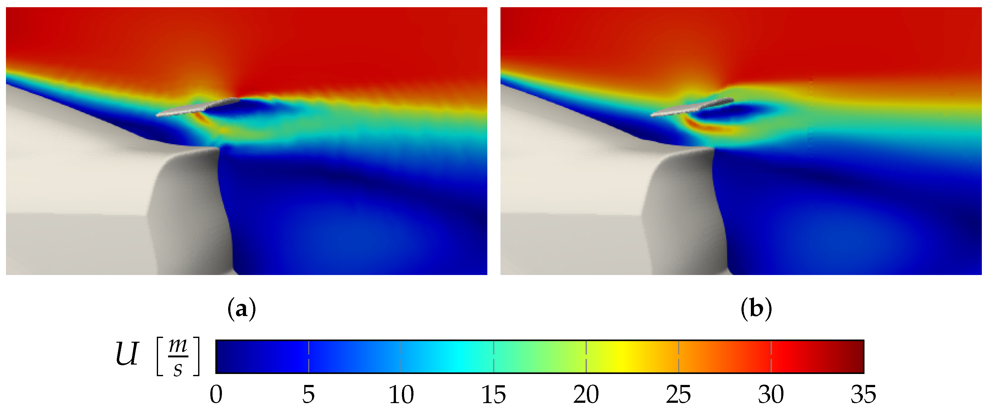
The final analysis of oPOD is a comparison against an alternative approach on modeling the discontinuous spoiler parameter . In this approach, a domain with a fixed mesh on which the solutions of the snapshots are mapped is used. As a consequence, the cells in the spoiler area occasionally are on the upper or lower side of the spoiler, depending on the snapshots parameter, or do feature a flow without spoiler at all. This can be problematic for the POD+I model since high nonlinearities of the modeled variables in the corresponding cells are introduced due to the fact that these cells are subject to high fluctuations compared with the parameters.
Figure 16 compares the alternative method for modeling discontinuous parameters with oPOD. Displayed in Figure 16a is the oPOD prediction for a solution with spoiler. It can be seen that the stagnation point in the front as well as the separation point at the trailing edge of the spoiler are accurately modeled. Moreover, the recirculation area beneath the spoiler is closely attached to the spoiler geometry. For the alternative approach, the model struggles with predicting these specific features, as the nonlinearities in the cells are too severe.
5. Conclusions
A novel method for handling discontinuous parameters for POD+I ROMs is presented. The steps involved are discussed and the method is demonstrated for two use cases. The industrial DrivAer use case shows significant improvements compared with an alternative way of modeling discontinuous parameters. It is possible to perform complex geometry transformation in the vicinity of static walls without degrading the CFD mesh. The oPOD prediction errors for the analytic use case are 30 times smaller compared with the POD+I method. This is due to the introduction of the transforming subdomains, which reduces the nonlinearities from the model perspective considerably (analogous to the shifted POD [17] method). In case of incomplete data due to oPOD subdomain transformations, an improved snapshot reconstruction method is proposed. It is shown that for the analytic use case the error only slightly increases with an increase in missing data. Compared with the standard POD+I method, the error is ten times smaller for an equivalent of missing data. The DrivAer as well as the analytic use case make use of a discontinuous parameter which is seamlessly included in the newly proposed oPOD method.
The demonstrated results motivate further research. Possible fields could focus on automatically setting up the oPOD subdomains. Currently, this is a manual task and human insight is required to determine the oPOD subdomain bounds. A future method could automatically detect the errors introduced at the subdomain bounds and resize the subdomains accordingly or regulate the size of the interpolation region. Moreover, a classification for various use cases could be of interest to further increase the robustness of the new method.
Funding
This research received no external funding.
Institutional Review Board Statement
Not applicable.
Informed Consent Statement
Not applicable.
Data Availability Statement
Not applicable.
Acknowledgments
This paper has benefited greatly from the comments and help of the author’s colleagues Matthias Bauer, Jakob Lohse and Marcel Staats.
Conflicts of Interest
The author declares no conflict of interest.
Abbreviations
The following abbreviations are used in this manuscript:
| CFD | Computational fluid dynamics |
| DD-POD | Domain-Decomposition POD |
| FOM | Full-order model |
| oPOD | Overset POD |
| POD | Proper orthogonal decomposition |
| POD+I | POD with interpolation |
| ROM | Reduced-order model |
| RANS | Reynolds-averaged Navier-Stokes |
| RBF | Radial basis function |
References
- Salmoiraghi, F.; Ballarin, F.; Corsi, G.; Mola, A.; Tezzele, M.; Rozza, G. Advances in geometrical parametrization and reduced order models and methods for computational fluid dynamics problems in applied sciences and engineering: Overview and perspectives. In Proceedings of the VII European Congress on Computational Methods in Applied Sciences and Engineering, Crete, Greece, 5–10 June 2016; Volume 1, pp. 1013–1031. [Google Scholar]
- Zimmermann, R.; Vendl, A.; Görtz, S. Reduced-order modeling of steady flows subject to aerodynamic constraints. AIAA J. 2014, 52, 255–266. [Google Scholar] [CrossRef] [Green Version]
- Jiang, G.; Kang, M.; Cai, Z.; Wang, H.; Liu, Y.; Wang, W. Online reconstruction of 3D temperature field fused with POD-based reduced order approach and sparse sensor data. Int. J. Therm. Sci. 2022, 175, 107489. [Google Scholar] [CrossRef]
- Sirovich, L. Turbulence and the dynamics of coherent structures. III. Dynamics and scaling. Q. Appl. Math. 1987, 45, 583–590. [Google Scholar] [CrossRef] [Green Version]
- Orr, M.J. Introduction to Radial Basis Function Networks. 1996. Available online: https://faculty.cc.gatech.edu/~isbell/tutorials/rbf-intro.pdf (accessed on 6 January 2022).
- Tan, B.T.; Willcox, K.E.; Damodaran, M. Applications of Proper Orthogonal Decomposition for Inviscid Transonic Aerodynamics. 2003. Available online: https://dspace.mit.edu/handle/1721.1/3694 (accessed on 22 January 2022).
- Salmoiraghi, F.; Scardigli, A.; Telib, H.; Rozza, G. Free-form deformation, mesh morphing and reduced-order methods: Enablers for efficient aerodynamic shape optimisation. Int. J. Comput. Fluid Dyn. 2018, 32, 233–247. [Google Scholar] [CrossRef]
- Nagy, P.; Fossati, M. Adaptive Data-Driven Model Order Reduction for Unsteady Aerodynamics. Fluids 2022, 7, 130. [Google Scholar] [CrossRef]
- De Boer, A.; Van der Schoot, M.S.; Bijl, H. Mesh deformation based on radial basis function interpolation. Comput. Struct. 2007, 85, 784–795. [Google Scholar] [CrossRef]
- Dwight, R.P. Robust mesh deformation using the linear elasticity equations. In Computational Fluid Dynamics 2006; Springer: Berlin/Heidelberg, Germany, 2009; pp. 401–406. [Google Scholar]
- Curless, B.; Levoy, M. A volumetric method for building complex models from range images. In Proceedings of the 23rd Annual Conference on Computer Graphics and Interactive Techniques, New Orleans, LA, USA, 4–9 August 1996; pp. 303–312. [Google Scholar]
- Quammen, C.; Weigle, C.; Taylor, R. Boolean operations on surfaces in vtk without external libraries. Insight J. 2011, 797, 1–12. [Google Scholar] [CrossRef]
- Löhner, R. Robust, vectorized search algorithms for interpolation on unstructured grids. J. Comput. Phys. 1995, 118, 380–387. [Google Scholar] [CrossRef]
- Guttman, A. R-trees: A dynamic index structure for spatial searching. In Proceedings of the 1984 ACM SIGMOD International Conference on Management of Data, Boston, MA, USA, 18–21 June 1984; pp. 47–57. [Google Scholar]
- Farrell, P.; Maddison, J. Conservative interpolation between volume meshes by local Galerkin projection. Comput. Methods Appl. Mech. Eng. 2011, 200, 89–100. [Google Scholar] [CrossRef]
- Benner, P.; Schilders, W.; Grivet-Talocia, S.; Quarteroni, A.; Rozza, G.; Miguel Silveira, L. Model Order Reduction: Volume 2: Snapshot-Based Methods and Algorithms; De Gruyter: Berlin, Germany, 2020. [Google Scholar]
- Reiss, J.; Schulze, P.; Sesterhenn, J.; Mehrmann, V. The shifted proper orthogonal decomposition: A mode decomposition for multiple transport phenomena. SIAM J. Sci. Comput. 2018, 40, A1322–A1344. [Google Scholar] [CrossRef] [Green Version]
- Schöberl, J.; Zulehner, W. On Schwarz-type smoothers for saddle point problems. Numer. Math. 2003, 95, 377–399. [Google Scholar] [CrossRef]
- Sobester, A.; Forrester, A.; Keane, A. Engineering Design via Surrogate Modelling: A Practical Guide; John Wiley & Sons: Hoboken, NJ, USA, 2008. [Google Scholar]
- Zimmermann, R. Gradient-enhanced surrogate modeling based on proper orthogonal decomposition. J. Comput. Appl. Math. 2013, 237, 403–418. [Google Scholar] [CrossRef] [Green Version]
- Fossati, M.; Habashi, W.G. Multiparameter analysis of aero-icing problems using proper orthogonal decomposition and multidimensional interpolation. AIAA J. 2013, 51, 946–960. [Google Scholar] [CrossRef]
- LeGresley, P.; Alonso, J. Investigation of non-linear projection for pod based reduced order models for aerodynamics. In Proceedings of the 39th Aerospace Sciences Meeting and Exhibit, Reno, NV, USA, 8–11 January 2001; p. 926. [Google Scholar]
- Zimmermann, R.; Görtz, S. Improved extrapolation of steady turbulent aerodynamics using a non-linear POD-based reduced order model. Aeronaut. J. 2012, 116, 1079–1100. [Google Scholar] [CrossRef]
- Lucia, D.J.; Beran, P.S.; Silva, W.A. Reduced-order modeling: New approaches for computational physics. Prog. Aerosp. Sci. 2004, 40, 51–117. [Google Scholar] [CrossRef] [Green Version]
- Everson, R.; Sirovich, L. Karhunen–Loeve procedure for gappy data. JOSA A 1995, 12, 1657–1664. [Google Scholar] [CrossRef] [Green Version]
- Mrosek, M.; Othmer, C.; Radespiel, R. Reduced-order modeling of vehicle aerodynamics via proper orthogonal decomposition. SAE Int. J. Passeng. Cars-Mech. Syst. 2019, 12, 225–237. [Google Scholar] [CrossRef]
- Heft, A.I.; Indinger, T.; Adams, N.A. Introduction of a New Realistic Generic Car Model for Aerodynamic Investigations; Technical Report, SAE Technical Paper; Technische Universität München: München, Germany, 2012; Available online: https://www.sae.org/publications/technical-papers/content/2012-01-0168/ (accessed on 22 January 2022).
- Jasak, H.; Jemcov, A.; Tukovic, Z. OpenFOAM: A C++ library for complex physics simulations. In Proceedings of the International Workshop on Coupled Methods in Numerical Dynamics, IUC, Dubrovnik, Croatia, 19–21 September 2007. [Google Scholar]
- Halton, J.H. On the efficiency of certain quasi-random sequences of points in evaluating multi-dimensional integrals. Numer. Math. 1960, 2, 84–90. [Google Scholar] [CrossRef]
Figure 1.
Schematic airfoil and flap CFD use case with parameters. (a) Airfoil for . (b) Airfoil and flap for .
Figure 1.
Schematic airfoil and flap CFD use case with parameters. (a) Airfoil for . (b) Airfoil and flap for .
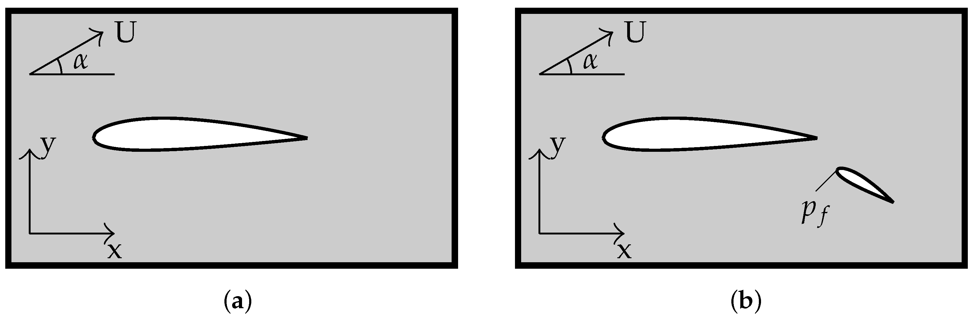
Figure 2.
Schematic mesh deformation of airfoil and flap use case. (a) Small distance between airfoil and flap. (b) Large distance between airfoil and flap.
Figure 2.
Schematic mesh deformation of airfoil and flap use case. (a) Small distance between airfoil and flap. (b) Large distance between airfoil and flap.
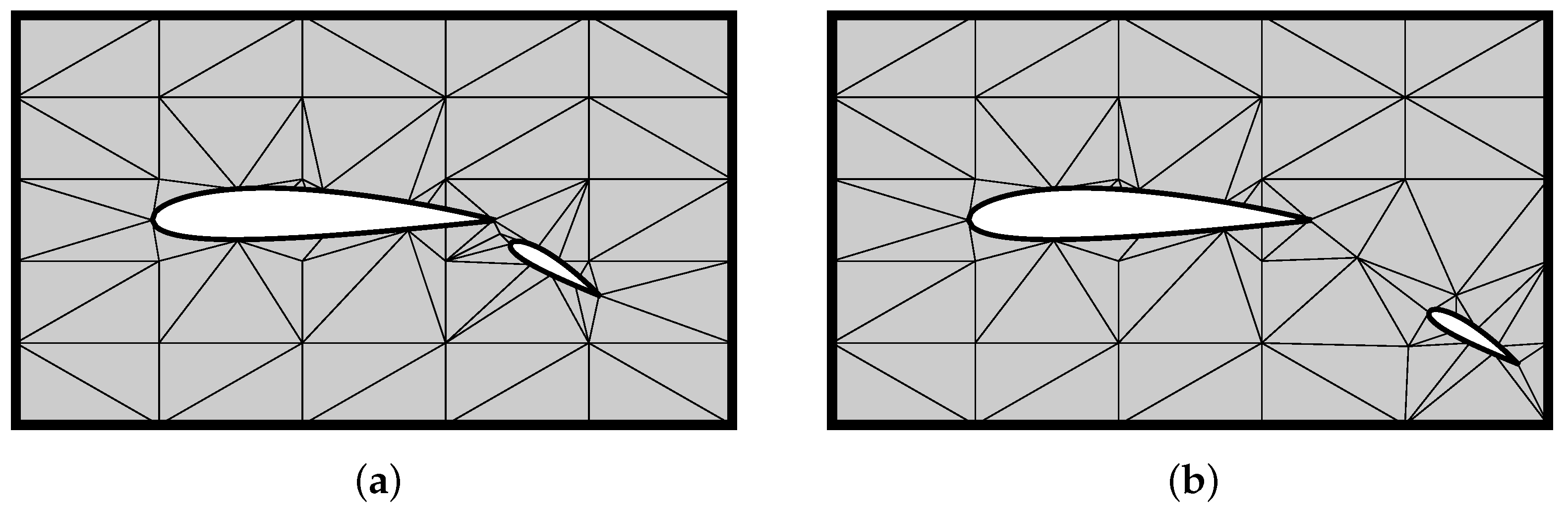
Figure 3.
oPOD example domain specification for varying parameter . (a) Airfoil for . (b) Airfoil and flap for .
Figure 3.
oPOD example domain specification for varying parameter . (a) Airfoil for . (b) Airfoil and flap for .
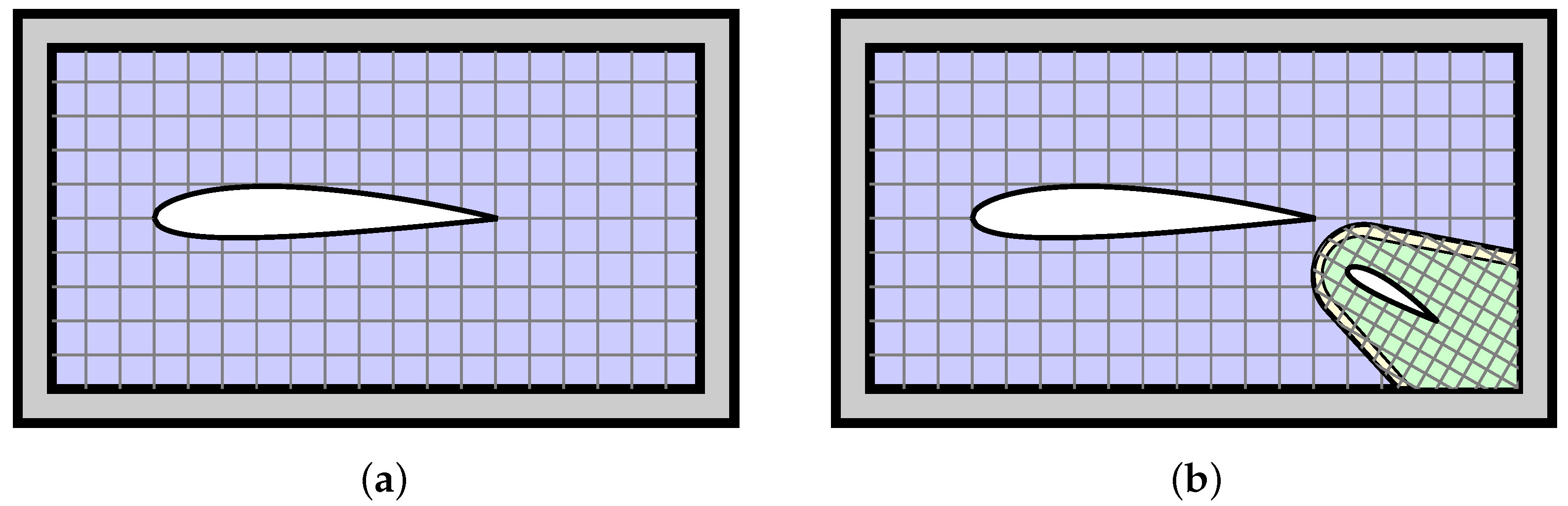
Figure 4.
Flowchart for the computation of the oPOD subdomain POD+I models. (a) Computation of the oPOD subdomain POD+I model. (b) Transformation and mapping of oPOD subdomain reference grid to a specific CFD snapshot.
Figure 4.
Flowchart for the computation of the oPOD subdomain POD+I models. (a) Computation of the oPOD subdomain POD+I model. (b) Transformation and mapping of oPOD subdomain reference grid to a specific CFD snapshot.

Figure 5.
Resulting snapshots for background and foreground model of the analytic test case. (a) Resulting snapshots with parameter . (b) Resulting snapshots with parameter .
Figure 5.
Resulting snapshots for background and foreground model of the analytic test case. (a) Resulting snapshots with parameter . (b) Resulting snapshots with parameter .

Figure 6.
prediction errors in the parameter space for POD+I and oPOD for . Samples of ROMs are marked with •. (a) error for POD+I. (b) error oPOD.
Figure 6.
prediction errors in the parameter space for POD+I and oPOD for . Samples of ROMs are marked with •. (a) error for POD+I. (b) error oPOD.

Figure 7.
Comparison of available data for full model data and incomplete model data. (a) Full model data snapshot set for . (b) Incomplete model data snapshot set for .
Figure 7.
Comparison of available data for full model data and incomplete model data. (a) Full model data snapshot set for . (b) Incomplete model data snapshot set for .
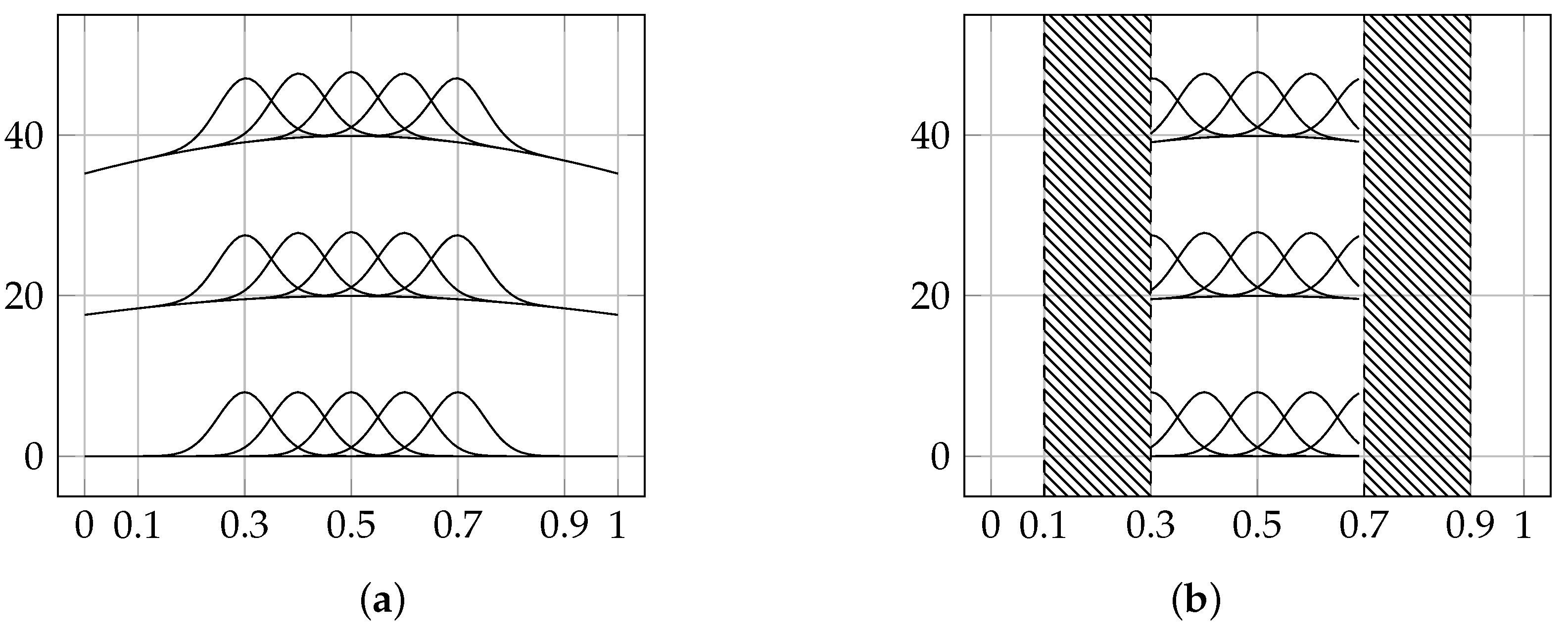
Figure 8.
Process with POD+I and oPOD predictions for . (a) Complete domain. (b) oPOD model interpolation.
Figure 8.
Process with POD+I and oPOD predictions for . (a) Complete domain. (b) oPOD model interpolation.
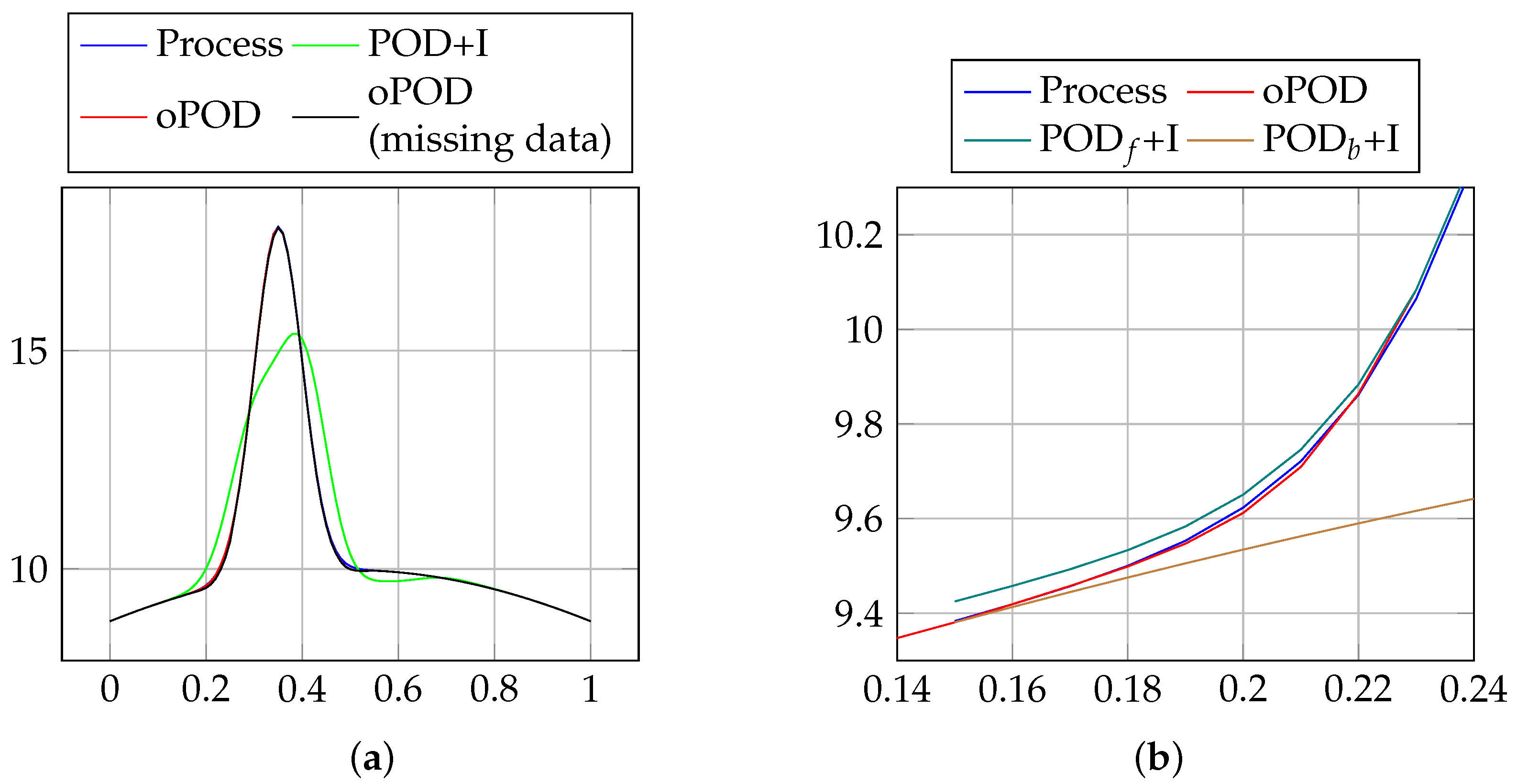
Figure 9.
prediction errors in the parameter space for oPOD with and without snapshot reconstruction for . Samples of oPODs are marked with •. (a) oPOD error without snapshot reconstruction. (b) oPOD error with snapshot reconstruction.
Figure 9.
prediction errors in the parameter space for oPOD with and without snapshot reconstruction for . Samples of oPODs are marked with •. (a) oPOD error without snapshot reconstruction. (b) oPOD error with snapshot reconstruction.
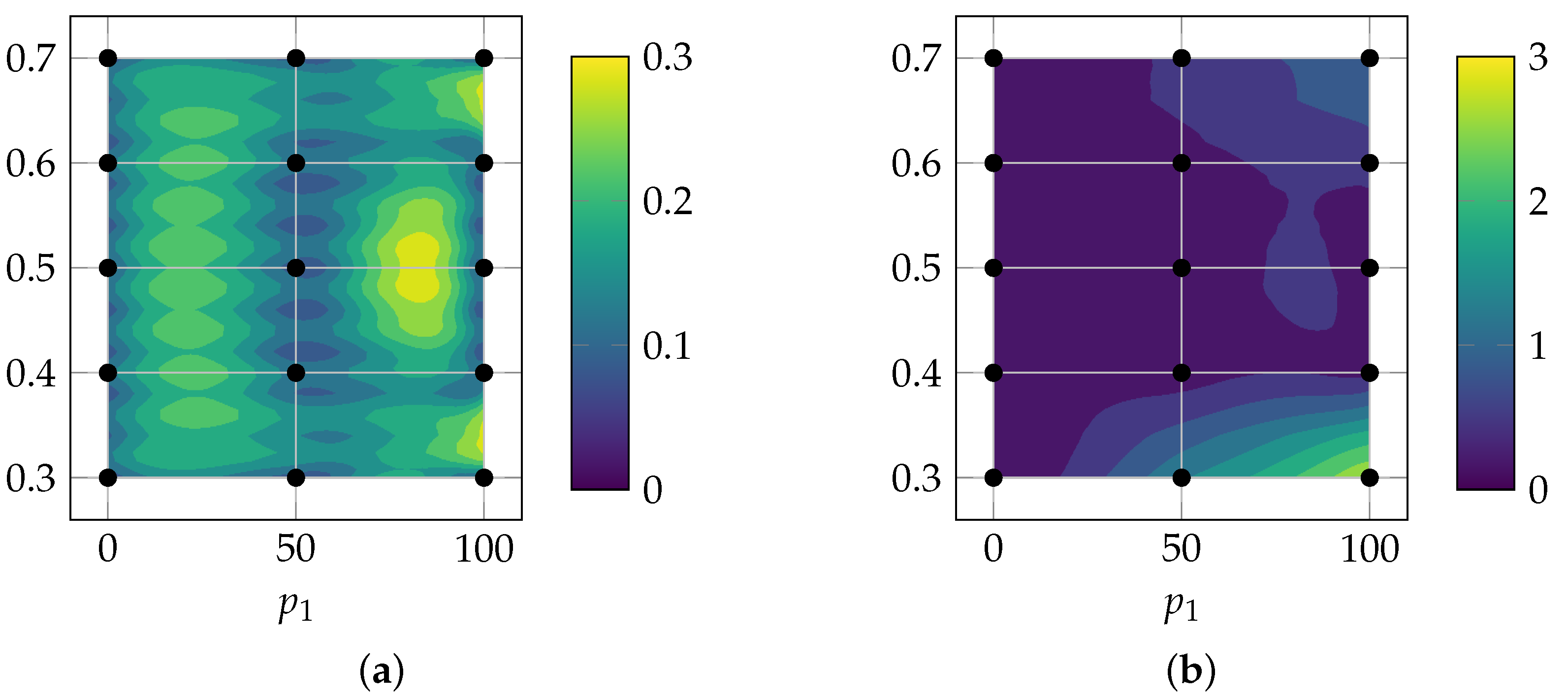
Figure 10.
prediction errors in the parameter space for oPOD foreground POD+I with increasing snapshot reconstruction size for .
Figure 10.
prediction errors in the parameter space for oPOD foreground POD+I with increasing snapshot reconstruction size for .

Figure 11.
Parameter variation for the DrivAer test case. (a) Minimal DrivAer body parameter values. (b) Maximal DrivAer body parameter values.
Figure 11.
Parameter variation for the DrivAer test case. (a) Minimal DrivAer body parameter values. (b) Maximal DrivAer body parameter values.

Figure 12.
oPOD domain decomposition and signed differences for the DrivAer use case. (a) oPOD domain decomposition. (b) Signed distance field slice of the foreground model.
Figure 12.
oPOD domain decomposition and signed differences for the DrivAer use case. (a) oPOD domain decomposition. (b) Signed distance field slice of the foreground model.
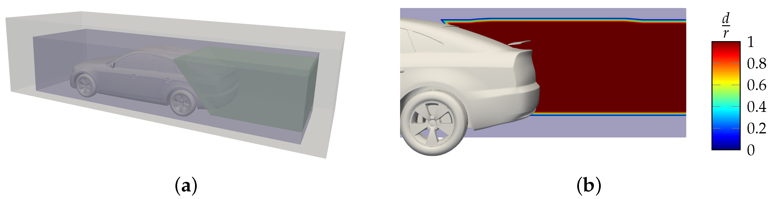
Figure 13.
CFD solutions and oPOD predictions for U at with and without spoiler. (a) CFD solution for U with spoiler. (b) oPOD prediction for U with spoiler. (c) CFD solution for U without spoiler. (d) oPOD prediction for U without spoiler.
Figure 13.
CFD solutions and oPOD predictions for U at with and without spoiler. (a) CFD solution for U with spoiler. (b) oPOD prediction for U with spoiler. (c) CFD solution for U without spoiler. (d) oPOD prediction for U without spoiler.

Figure 14.
CFD solutions and oPOD predictions for at with and without spoiler. (a) CFD solution for with spoiler. (b) oPOD prediction for with spoiler. (c) CFD solution for without spoiler. (d) oPOD prediction for without spoiler.
Figure 14.
CFD solutions and oPOD predictions for at with and without spoiler. (a) CFD solution for with spoiler. (b) oPOD prediction for with spoiler. (c) CFD solution for without spoiler. (d) oPOD prediction for without spoiler.
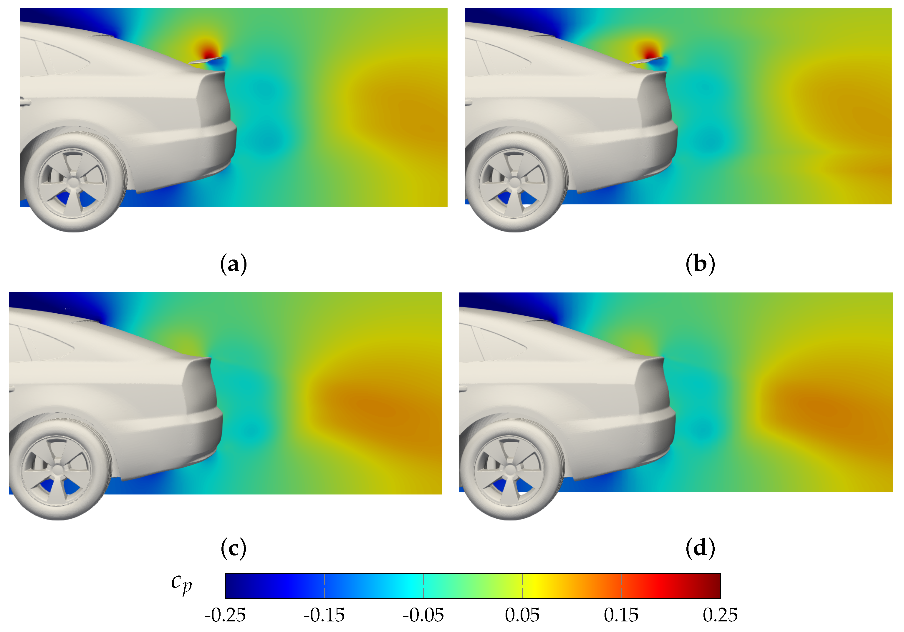
Figure 15.
Influence of oPOD interpolation region. (a) oPOD prediction with interpolation. (b) oPOD prediction without interpolation.
Figure 15.
Influence of oPOD interpolation region. (a) oPOD prediction with interpolation. (b) oPOD prediction without interpolation.

Figure 16.
Comparison of oPOD prediction with alternative POD+I prediction. (a) oPOD prediction close up. (b) Alternative POD+I close up.
Figure 16.
Comparison of oPOD prediction with alternative POD+I prediction. (a) oPOD prediction close up. (b) Alternative POD+I close up.
Publisher’s Note: MDPI stays neutral with regard to jurisdictional claims in published maps and institutional affiliations. |
© 2022 by the author. Licensee MDPI, Basel, Switzerland. This article is an open access article distributed under the terms and conditions of the Creative Commons Attribution (CC BY) license (https://creativecommons.org/licenses/by/4.0/).
Share and Cite
MDPI and ACS Style
Karcher, N. POD-Based Model-Order Reduction for Discontinuous Parameters. Fluids 2022, 7, 242. https://doi.org/10.3390/fluids7070242
AMA Style
Karcher N. POD-Based Model-Order Reduction for Discontinuous Parameters. Fluids. 2022; 7(7):242. https://doi.org/10.3390/fluids7070242
Chicago/Turabian StyleKarcher, Niklas. 2022. "POD-Based Model-Order Reduction for Discontinuous Parameters" Fluids 7, no. 7: 242. https://doi.org/10.3390/fluids7070242