
An Application of Kolmogorov Complexity and Its Spectrum to Positive Surges


1
Department of Structures for Engineering and Architecture, University of Napoli Federico II, Via Claudio 21, 80125 Napoli, Italy
2
Faculty of Technical Sciences, University of Novi Sad, Dositeja Obradovića Sq. 1, 21000 Novi Sad, Serbia
3
Department of Physics, Faculty of Sciences, University of Novi Sad, Dositej Obradovic Sq. 3, 21000 Novi Sad, Serbia
*
Author to whom correspondence should be addressed.
Fluids 2022, 7(5), 162; https://doi.org/10.3390/fluids7050162
Submission received: 13 January 2022
/
Revised: 27 April 2022
/
Accepted: 3 May 2022
/
Published: 6 May 2022
Abstract
:A positive surge is associated with a sudden change in flow that increases the water depth and modifies flow structure in a channel. Positive surges are frequently observed in artificial channels, rivers, and estuaries. This paper presents the application of Kolmogorov complexity and its spectrum to the velocity data collected during the laboratory investigation of a positive surge. Two types of surges were considered: a undular surge and a breaking surge. For both surges, the Kolmogorov complexity (KC) and Kolmogorov complexity spectrum (KCS) were calculated during the unsteady flow (US) associated with the passage of the surge as well as in the preceding steady-state (SS) flow condition. The results show that, while in SS, the vertical distribution of KC for Vx is dominated by the distance from the bed, with KC being the largest at the bed and the lowest at the free surface; in US only the passage of the undular surge was able to drastically modify such vertical distribution of KC resulting in a lower and constant randomness throughout the water depth. The analysis of KCS revealed that Vy values were peaking at about zero, while the distribution of Vx values was related both to the elevation from the bed and to the surge type. A comparative analysis of KC and normal Reynold stresses revealed that these metrics provided different information about the changes observed in the flow as it moves from a steady-state to an unsteady-state due to the surge passage. Ultimately, this preliminary application of Kolmogorov complexity measures to a positive surge provides some novel findings about such intricate hydrodynamics processes.
1. Introduction
Positive surges are frequently observed in both artificial and natural channels. In channels used for irrigation and water energy production, a positive surge may be created by a partial or complete closure of a gate, causing a sudden increase in flow depth [1,2]. In natural channels, tidal bores are characteristic of the rivers and estuaries of Europe, China, Australia, and South America, such as the Seine, Garonne, Severn, Elbe, Qiantang, and Amazon, while Tsunami-induced bores were also observed [3]. The waves associated with a tidal bore propagate upstream, rapidly increasing the free-surface profile as the tidal flow turns to rising. Bores are formed when the tidal range exceeds 4.5 to 6 m, and the tidal wave is amplified by the funnel shape of the river mouth and the lower estuarine zone [3]. Despite the fact that they are sometimes seen as a tourist attraction, tidal bores can be very dangerous as they can adversely impact the local natural ecosystems (large sediment resuspension, impairment of aquatic organisms and fish reproduction and development), severely damage local infrastructures (bridges, roads, levees, etc.), and more generally hinder the development of local resources [3].
In laboratory flumes, positive surges are studied upon the Froude similitude, because field and laboratory data demonstrated that the characteristics of a surge are related to its inflow Froude number Fr1. If the Froude number ranges from 1 to approximately 1.5, the surge is followed by a train of quasi-periodic secondary waves and is called undular [3]. On the other hand, a maximum in wave amplitude and steepness was found for Fr1 = 1.4 to 1.5, which was associated with some breaking and air entrainment at the first wave crest. If the Froude number is larger, the surge has a breaking front with a roller, and hence it is termed a breaking or weak surge [3].
After the first pioneering studies [4,5,6], several researchers investigated the positive surges and tidal bores [7,8,9,10,11]. While older studies were limited to visual observations and sometimes free-surface measurements [12,13,14], in the last two decades unsteady turbulence, air entrainment, and sediment transport characteristics were measured using particle image velocimetry (PIV) and acoustic Doppler velocimetry (ADV) in the laboratory [15,16,17] and in the field [18,19]. Finally, numerical studies on tidal bores, both with Large Eddy Simulation (LES) and Smoothed Particles Hydrodynamics (SPH) approaches, focused on the prediction of unsteady flow free-surface dynamics and velocity distribution, where the requirement for high-quality datasets for the validation of the numerical results remains imperative [20,21,22].
Turbulent flows are defined and characterized by irregularity, diffusivity, large Reynolds numbers, 3D vorticity fluctuations, and dissipation [23]. Irregularity or randomness cannot be measured using a deterministic approach, but it can only be reliably measured using statistical methods [23]. Complexity measures were previously used for the extraction of information, such as environmental time series (cosmic rays, solar and UV radiation) [24], biomedical signals [25,26], testing of random number generators, etc., from data. In the last decade, such measures, namely the Kolmogorov complexity, were applied to study the randomness of turbulent environmental fluid mechanic (EFM) flows [27], such as the flow series and regimes [28,29] and different types of open channel flows [30,31,32].
This paper presents the results of the application of Kolmogorov complexity (KC) and Kolmogorov complexity spectrum (KCS) to the experimental velocity data of both an undular and breaking surge. The study aims at identifying how those two metrics of complexity can improve our current knowledge about positive surges. The manuscript is structured as follows. After some remarks about randomness, the Kolmogorov complexity and spectrum, as well as the concept of Information, are presented. Second, a short description of the laboratory experiments carried out to collect the velocity data and the procedure used to post-process such data to derive KC and KCS are presented. Then, some basic observations about the flow field during the surge passage are provided. After that, the results from this study in terms of KC and KCS are presented and discussed to identify some novel insights and limitations of the present research, and, finally, some conclusions are proposed.
2. Some Remarks about Randomness, Kolmogorov Complexity and Information
While a comprehensive mechanical theory of turbulence is still missing [27], the term randomness that is broadly used in different sciences dealing with fluids and randomness is also one of the fundamental characteristics of a turbulent flow.
While Ichimiya and Nakamura reviewed several definitions of randomness [33], Khrennikov [34] further developed the original definition of randomness proposed by Kolmogorov. He outlined three different interpretations of randomness: (i) randomness as unpredictability; (ii) randomness as typicality; and (iii) randomness as complexity. He noted that: “As we have seen, none of the three basic mathematical approaches to the notion of randomness (based on unpredictability, typicality, and algorithmic complexity) led to a consistent and commonly accepted theory of randomness”. Among these interpretations, only that from Kolmogorov is based upon the concept of complexity, but this viewpoint is not always accepted in our understanding of probability. Furthermore, Kolmogorov complexity is not even computable. Therefore, randomness is either a subjective measure or an objective measure that is non-computable. Following this discussion, we might conclude that randomness is not a mathematical notion, but rather a physical notion. Namely, it is the physical procedure where the true randomness is hidden. Therefore, mathematical methods might not be sufficient to theoretically establish the concept of randomness itself. Notably, in Kolmogorov’s approach there is “no room” in which the level of randomness can be placed.
Many scientific analyses use the term “algorithmic” randomness, which is directly related to the definition of complexity proposed by Kolmogorov [35]. Such metrics can be quantified by their algorithmic complexity, which is a measure of how long an algorithm would take to complete given an input of size n. This time bound should be finite and practical even for large values of n. Hence, complexity is calculated asymptotically as n approaches infinity as a measure of randomness.
It should be noted that in physical and engineering sciences, scientists often apply a heuristic technique to choose a model. To formulate a heuristic, we consider any approach to problem solving that uses a practical method that is not guaranteed to be optimal, but it is sufficient either to rapidly reach a goal or until a better approach is developed [36].
Complexity measures, such as Kolmogorov complexity and its derivatives, are information measures, i.e., they stem from algorithmic information theory, where information is broadly defined as the pattern of organization of mass and energy [37]. This definition relates the concept of information to any process of transfer of mass, momentum, or energy in any fluid and across any environmental interface [27]. Inherently, the concept of information includes all patterns of organization of matter and energy in the brains and bodies of human beings and animals. This information comes up from their genetic heritage and is further created by their interaction with the external and inner worlds and later recorded in their sensory, nervous, and biochemical systems. Thus, our subjective understanding of the world, which is embedded in our minds and feelings, can be regarded from the outer as a body of information as having that pattern of organization [37]. Interestingly, peripheral nerve fibers and neural pathways dedicated to conveying information from the body’s interior to the brain end in their own dedicated region, the insular cortex, whose activity patterns are perturbed by emotions [38].
3. Experimental Data
3.1. Channel Setup and Instrumentation
The experimental data used herein were collected in a horizontal tilting flume at the University of Queensland, previously by Chanson and co-workers [3,16,17]. The channel was 0.5 m wide and 12 m long, and it was made of a smooth PVC bed and glass walls. It was fed by a constant head tank, and the discharge was measured with orifice meters (accuracy < 2%). A tainter gate was located next to the downstream end, at x = 11.15 m from the channel intake, where x is the distance from the channel’s upstream end. Its controlled and rapid closure created a positive surge propagating upstream.
A constant flow rate (Q = 0.060 m3/s) was used in the experimental study. Instantaneous velocity before and during the propagation of the surge was measured with an acoustic Doppler velocimeter (ADV) Sontek™ 16MHz micro-ADV equipped with a 2D side-looking head. Water depth was measured, in steady flow, with rail-mounted pointer gauges and, in unsteady flow, using seven acoustic displacement meters (ADM) Microsonic™ Mic + 25/IU/TC. The ADV and the seven ADMs were located at x = 5 m and at x = 1.985 m, 2.995 m, 4 m, 5 m, 6 m, 9 m, and 10.9 m downstream the flume intake, respectively (Figure 1).
During the experiments, two different gate openings after closure hg were used leading to the formation of both undular (non-breaking) and breaking surges (Table 1). For both the steady and unsteady state conditions, for the ADV the velocity range was 1.0 m/s, the sampling rate was 50 Hz, and the data accuracy was 1% of the velocity range [16]. All measurements were carried out on the channel centerline. Further details about the experiments are presented in [16].
The velocity distribution was measured in the steady flow at x = 5 m. The results show that the inflow conditions were partially developed. The boundary-layer thickness was about δ/d0 = 0.265, where d0 is the initial flow depth (Table 1). The velocity data agreed with theoretical velocity profiles in the turbulent boundary layer and the experimental data collected in a large wind tunnel operating at comparable Reynolds numbers [39] (Figure 2). From the data best fit with the low law, the shear velocity was estimated: V* = 0.0375 m/s. The findings demonstrated that the flume was hydraulically smooth, and the flow was smooth turbulent.
3.2. Generation of the Surge
The surge was created using the following procedure. The flow was measured for at least 5 min in steady gradually varied conditions, which previous experiments demonstrated to be effective to achieve steady conditions [3]. Then, measurements and data acquisition started approximately 1.5 min before gate closure. The surge was created by the rapid (closure time < 0.2 s) partial closure of the downstream gate [16,20]. After the closure, the surge propagated upstream, and data acquisition ended when the bore front reached the channel inlet (Figure 1). In Table 1, the surge front celerity U was derived from the displacement meters data between x = 6 m and 4 m. Moreover, d0 was measured at x = 5 m, and dconj was calculated from the continuity and momentum equations. Note that the data in Table 1 for 60-6 and Run 60-7 are those derived from the average of 23 runs with the same gate opening but different vertical elevation z for the ADV system.
4. Kolmogorov Complexity and Spectrum: Past Applications and Calculation
4.1. Complexity Measures
Complexity measures, such as Kolmogorov complexity and its derivatives, can be used to provide the scientific community with new insights into the behavior of complex systems and processes that cannot be identified with traditional mathematical methods. Past studies have indicated that a large value of KC in solar radiation time series points out the presence of variable cloudiness [24], while, in biomedical studies, a large KC of measurements (heart rate, respiration rate, etc.) might indicate a particular stage of sleep-apnea [25,26], and, if the KC is larger, the neuron activity is more disordered. Thus, a decrease in the KC complexity in the tasking state might be related to the increase in neuronal activity synchronization [26]. Furthermore, low values of KC for the streamflow time series in rivers are often due to human activity, such as urbanization, drainage, irrigation, etc. [28,29].
In open channel turbulent flows, the approach based upon complexity measures was already applied. Mihailović et al. [30] quantified the randomness of turbulent velocity data measured in laboratory canopy flows with different densities of vegetation using Kolmogorov complexity and Kolmogorov complexity spectrum and found that KC was related to the size of the eddies and the coherent structures of the flow. Sharma et al. [31] applied those complexity metrics to the experimental velocity data collected in an alluvial channel with and without downward seepage. They identified larger values of KC and higher randomness in the flow with seepage. This result was confirmed by the spectral analysis of the velocity time series. Lade et al. [32] explored the effect of a mining pit on the randomness of a turbulent flow around the pier using KC and KCS. They comparatively considered two cases: one where only a pier was placed in the channel and the second where a rectangular mining pit was excavated upstream of the pier. They found that the pit excavation increased both KC and KCS around the pier, suggesting an increased degree of randomness associated with the pit in the channel. In the end, these studies demonstrated the potential of complexity measures to identify patterns of turbulence in complex open-channel flows.
In the present study, both metrics, i.e., Kolmogorov complexity and the Kolmogorov Complexity Spectrum, were calculated for the velocity field in the open-channel flow both in a steady state (before the formation of the surge) and in an unsteady state (during the passage of the surge).
4.2. Kolmogorov Complexity
If X is the flow velocity, and x is its specific value, we can define the Kolmogorov complexity KC (x) of an object x as the length, in bits, of the smallest program that can be run on a universal Turing machine U and that prints object x. However, the complexity KC (x) cannot be directly computed for an arbitrary object x. Hence, we need to approximate KC using a binary object x, which is compressed, and the size of the compressed object is associated with the Kolmogorov complexity.
In the present study, the Lempel and Ziv Algorithm (LZA) [40] was applied for calculating the KC of a time series. The calculation of the KC of a time series X(x1, x2, x3, …, xN) using the LZA algorithm includes the following steps:
- (1)
- the time series are encoded by creating a sequence S of the characters 0 and 1 written as s(i) = 1, 2, …, N according to the rule s(i) = 0 if xi < xt or s(i) = 1 if xi > xt, where xt a threshold value. The threshold is often selected as the mean value of the time series, while other encoding schemes are also available [28];
- (2)
- the complexity counter c(N), which is the minimum number of distinct patterns contained in a sequence of characters, is computed. The complexity counter c(N), is a function of the sequence length, N, bounded by b(N) = N/log2N, as it approaches infinity, i.e., c(N) = O (b(N));
- (3)
- the normalized information measure Ck (N), which is , is calculated. For a nonlinear time series, Ck (N) ranges from 0 to 1, although it can be larger than 1 for random finite-size sequences.
4.3. Kolmogorov Complexity Spectrum
It should be acknowledged that the application of Kolmogorov complexity has two shortcomings: (1) this metric is not able to distinguish between time series with different amplitude variations and those with similar random components (it depends on structure of a time series); and (2) in the procedure of binarization of a time series, its complexity is not explicitly seen in the rules of the applied procedure. Hence, it should be acknowledged that, when threshold coding is identified, some information about the composition of time series might be lost. This shortcoming suggested to apply in the present study also the Kolmogorov complexity spectrum metric, which is described in [30].
The procedure for the calculation of the KCS C (c1, c2, c3, …, cN) for a time series X(x1, x2, x3, …, xN) is presented in Figure 3. Using the KCS, the range of amplitudes in a time series that represents a complex system with highly enhanced stochastic components can be systematically investigated. The KCS considers the aforementioned issues in computing the KC, as it calculates the complexity of taking each element of the series as a threshold value. In the end, this relates to the probability distribution with compressibility.
5. Results
5.1. Time-Variable Depth and Velocity Field
Figure 4 and Figure 5 show the effects of the undular surge (Run 60-7) and the breaking surge (Run 60-6), respectively, on the velocity field at two vertical dimensionless elevations z/d0, close to the bed and the free surface, respectively. Those elevations were chosen as they reflect some differences in the streamwise velocity close to the bed between the undular surge and the breaking surge. Note that z = z′ + ADV measurement volume, where z′ is the elevation from the bed of the measurement point. Each plot presents the distribution against the dimensionless time t × (g/d0)0.5 of the dimensionless velocities Vx/V* and Vy/V* and water depth d/d0. Note that Vx and Vy are the longitudinal and horizontal transverse velocity components, respectively. They are assumed to be positive downstream and towards the left wall, respectively. In the plots, the zero dimensionless time corresponds to a time placed 10.0 s before to the first wave crest passage at the sampling location.
Velocity data were filtered using a cutoff frequency, such that the averaging time is greater than the characteristic period of fluctuations and smaller than the characteristic period for the time-evolution of the mean properties. In the undular surge, Eulerian flow properties showed an oscillating pattern with a period of ranging from 1.01 to 1.87 s that corresponded to the period of the free-surface undulations. The unsteady data were therefore filtered with a low/high-pass filter threshold greater than 0.99 Hz (i.e., 1/1.01 s) and smaller than the Nyquist frequency (herein 25 Hz). Following previous studies [3,19], the cutoff frequency was selected as 1 Hz. The same filtering technique was applied to both longitudinal and transverse velocity components for both the undular and the breaking surges.
In the undular surge (Run 60-7), Vx sharply decreased with the passage of the first wave crest and later oscillated with the same period as, but out of phase with, the free-surface undulations (Figure 4). The maximum and minimum velocities were observed below the wave troughs and crests, respectively. This trend was seen at all vertical locations. In the upper flow region, above z/d0 = 0.50, fluctuations for both velocity components were observed beneath the undulations, but Vx was always positive (Figure 4).
In the breaking surge (Run 60-6), as the water level gently raised, Vx rapidly decreased for at both z′ = 100 mm and z′ = 0.00 mm. Immediately after, the passage of the positive surge roller was associated with a sharp increase in the free-surface elevation corresponding with a discontinuity in terms of the water depth. Such an increase in the water depth corresponded to a rapid deceleration to a slower flow motion to satisfy mass conservation (Figure 5). Notably, at the same relative elevation z/d0, the rate of flow deceleration in the breaking surge was larger than that in the undular surge (Figure 4a and Figure 5a). No significant patterns were observed for the transverse velocity Vy/V*, which was seen to fluctuate around 0.
Second, the vertical elevation z affected the temporal distribution of the velocity (Figure 5). At the larger depth, i.e., z/d0 > 0.3, Vx decreased rapidly at the surge front but remained positive (Figure 5b). On the contrary, for z/d0 < 0.3, for a dimensionless time t × (g/d0)0.5 from 86 to 106, Vx values were negative with a minimum value of (Vx/V*)min = −2.35 (Figure 5a). Such a sudden longitudinal flow reversal revealed an unsteady flow separation below the surge front. This finding is consistent with previous studies in both the laboratory and the field on positive surges [3,18], and it is believed to impact the local suspended sediment processes and ecology [18]. During all experiments, both velocity components were seen to fluctuate beneath the surge and in the flow field behind the surge. For both undular and breaking surges, large temporal variations of the longitudinal and transverse velocity components were seen at all vertical elevations.
5.2. Reynolds Stresses
A Reynolds stress tensor component equals the fluid density times the cross-product of turbulent velocity fluctuations, which is the deviation of the instantaneous velocity from an average velocity component, which in unsteady flow is the low-pass filtered velocity component. Filtered velocity data were used to calculate the velocity fluctuations and finally to obtain the Reynolds stresses.
Figure 6 shows the vertical distribution of the dimensionless normal Reynolds stresses in the undular surge (Run 60-7) for the longitudinal velocity component Vx (Figure 6a) and the horizontal transverse velocity Vy (Figure 6b), respectively, in both steady-state (SS) and unsteady-state (US) conditions. For the SS, the median of the KC values of several time series which were 10 s long was considered.
Figure 6a shows that normal stresses for the Vx component were larger everywhere in an unsteady state (US) than in a steady state (SS). This is due to the intense normal stresses observed during the US beneath wave crests and just before each crest. Over the water depth, in SS, normal stresses were larger at the bed and rapidly decreased as the distance from the bed increased, but above z′ = 4.5 mm they were almost constant with the elevation from the bed. In US, normal stresses values increased as the distance from the bed increased. Such large turbulent stresses were already observed during the surge passage and the ensuing undulations, especially far from the channel bed [3]. For the transverse velocity component Vy (Figure 6b), normal stresses were, again, generally larger in US than is SS. The largest values were observed at the bed in SS. They sharply decreased with bed elevation, but, above z′ = 20 mm, they ranged from 0.15 to 0.30. In US, along the depth, normal stresses Vy2/V*2 were almost all in the range from 0.30 to 0.60.
Figure 7 shows the vertical distribution of the dimensionless normal Reynolds stresses in the breaking surge (Run 60-6) for the longitudinal velocity component Vx (Figure 7a) and the horizontal transverse velocity Vy (Figure 7b), respectively, in both SS and US conditions.
Normal stresses for the Vx component (Figure 7a) were generally larger in a steady state than those in an unsteady state. However, rather than at the bed, the difference between SS and US values was quite small. Over the depth, above z′ = 4.5 mm, the vertical distributions of Vx2/V*2 in both SS and US were almost constant, as the elevation from the bed increased. Even normal stresses for the Vy component (Figure 7b) were generally larger in SS than those in US. Again, contrary to measurements at the bed, the difference between SS and US values was small. In SS at the bed, a value of 0.9 was observed. Vy2/V*2 values rapidly decreased as the distance from the bed increased, and, above z′ = 20 mm, they were almost constant. In US, Vy2/V*2 values were almost constant over the depth.
5.3. Kolmogorov Complexity
For both surges and in both steady-state (SS) and unsteady-state (US) conditions, the Kolmogorov complexity was calculated at 24 different elevations from z′ = 0.00 mm (bed) to z′ = 110.00 mm.
Figure 8 shows the vertical distribution of the Kolmogorov complexity in the undular surge (Run 60-7) for the longitudinal velocity component Vx (Figure 8a) and the horizontal transverse velocity Vy (Figure 8b), respectively, in both SS and US conditions. For the SS, the median of the KC of several time series 10 s long was considered.
Figure 8a shows that the KC values for the Vx component were all larger in a steady state (SS) than in an unsteady state (US). Furthermore, over the water depth, they were almost constant and about 0.03 in US, while in SS they were generally decreasing as the distance from the bed, ranging from 0.18 to 0.03. Thus, in terms of KC, SS and US seemed to represent two distinctively different conditions for the longitudinal velocity. On the other side, for the transverse velocity component Vy (Figure 8b), the differences between SS and US were generally very minor close to the bed but much larger far from it. Furthermore, over the depth, in the KC values in SS KC ranged from 0.21 to 0.29, and large differences were observed in US (KC was from 0.10 to 0.27).
In the end, at any elevation, in both SS and US conditions, the KC associated with the transverse velocity was larger than that associated with the longitudinal velocity. Moreover, in an unsteady flow, the KC was almost constant for Vx and largely changing for Vy. This is consistent with the velocity data observed in Figure 4, where a sudden decrease and undular patterns were observed for Vx (and not for Vy) during the passage of the undular surge.
Figure 9 shows the vertical distribution of the Kolmogorov Complexity in the breaking surge (Run 60-6) for the longitudinal velocity component Vx (Figure 9a) and the horizontal transverse velocity Vy (Figure 9b), respectively, in both steady-state and unsteady-state conditions.
In SS flow, the KC values for Vx and Vy were, as expected, very similar to those for the undular surge. In US, the KC values for Vx (Figure 9a) in the breaking surge were quite differently distributed than those in the undular surge. They were not constant along the vertical but ranged from 0.03 to 0.13. Furthermore, they were generally decreasing as the distance from the bed increased. In US, for Vy (Figure 9b), the KC values ranged from 0.07 to 0.23. Again, as for the undular surge, in both SS and US conditions, the KC values for the transverse velocity were larger than those for the longitudinal velocity.
5.4. Kolmogorov Complexity Spectrum
The Kolmogorov complexity spectrum was computed for both surges at two vertical elevations, z′ = 0.00 mm and 100 mm, before and during the passage of the surge through the measurement point (x = 5 m downstream of the channel intake). The KCS distribution shows how the KC values are associated with the velocity values observed during the experiments identifying those characterized by the largest KC and randomness values.
Figure 10 shows the Kolmogorov complexity spectrum of Vx for both the undular and the breaking surge in SS and US conditions at two elevations from the bed, z′ = 0.00 mm and 100 mm. The widest KC spectra were associated with the breaking surge where very low and negative Vx velocities were found at 100 mm and at the bed, respectively.
For the undular surge, Vx was in the range from 0.29 to 0.88 m/s and from 0.36 to 0.97 m/s at z′ = 0.00 mm and 100 mm, respectively, while Vx for the breaking surge was in the range from −0.09 to 0.88 m/s and from 0.21 to 0.96 m/s at z′ = 0.00 mm and 100 mm, respectively. The breaking surge had peaks in KC at both z′ = 0.00 mm and 100 mm that were larger than those of the undular surge. At the bed, the largest KC was associated with both for the undular and the breaking surge to Vx = 0.72 m/s, while at z′ = 100.00 mm, it was found for 0.86 and 0.83 m/s for the undular and the breaking surge, respectively. The peak values were KC = 0.225 and 0.180 for the breaking surge at z′ = 100 mm and z′ = 0.00 mm, respectively. For the undular surge, the peak values were 0.219 and 0.174 at z′ = 100 mm and z′ = 0.00 mm, respectively. These larger peaks for the breaking surge confirm this type of surge is characterized by a randomness larger than the undular surge, in which the longitudinal velocity Vx followed an undular pattern associated with the free-surface undulations. In addition, for both surges, the lower values of KC corresponded to velocities lower than 0.60 and 0.70 m/s at z′ = 0.00 mm and 100 mm, respectively.
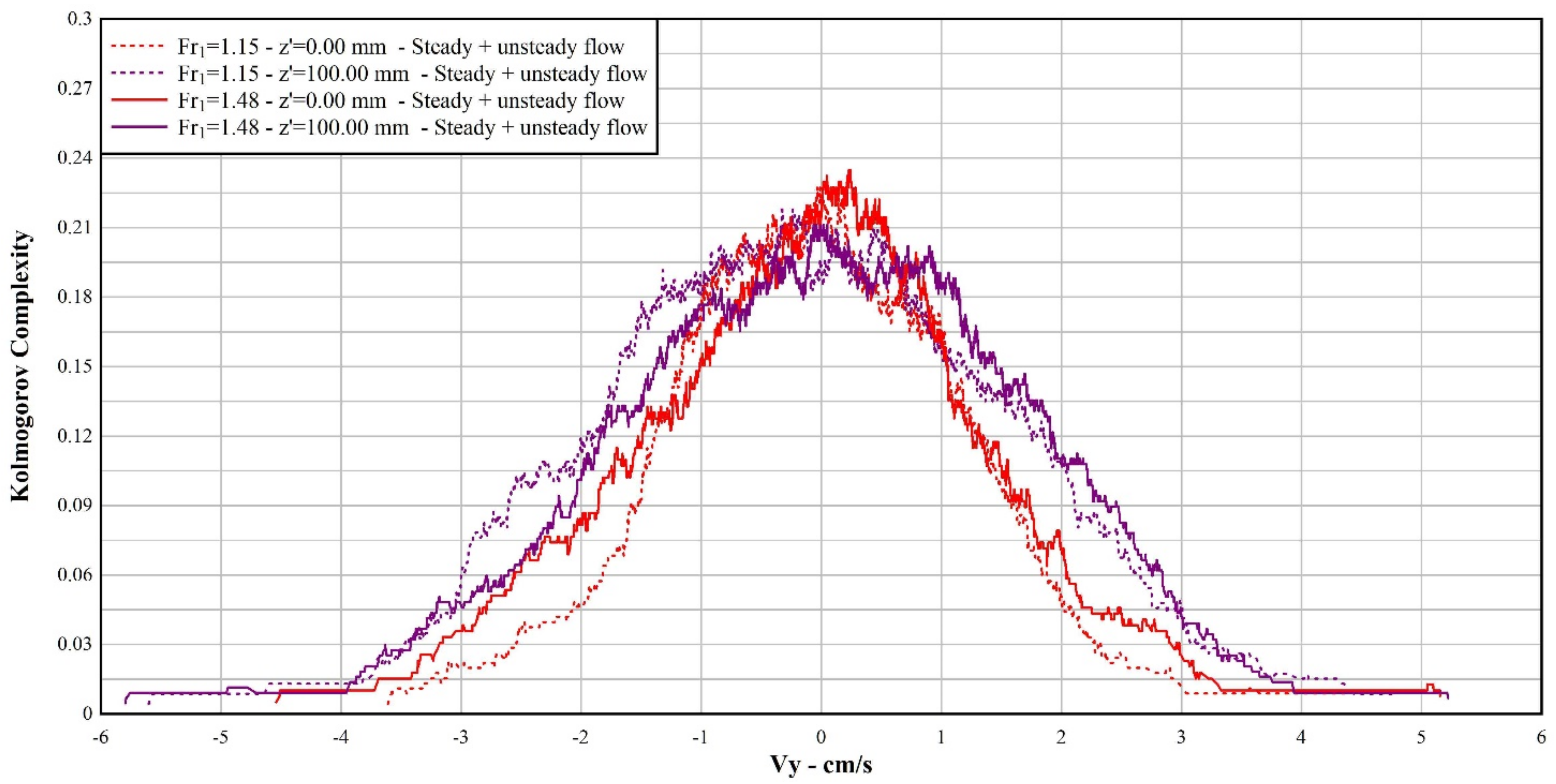
Figure 11 shows the Kolmogorov complexity spectrum of Vy for both the undular and the breaking surges in SS and US conditions at two elevations from the bed, z′ = 0.00 mm and 100 mm. At any elevation from the bed and for both for the undular and the breaking surge, the KC was found to peak about 0.00 m/s, which was where the KCS distribution was also centered. Both surges had a peak in KC at the bed, where KC was 0.225 and 0.235 for the undular surge and the breaking surge, respectively. At the elevation of z′ = 100.00 mm, the peak values for KC were 0.218 and 0.209, for the undular and the breaking surge, respectively.
In the end, for both surges, while the transverse velocity was seen to peak at the bed, the longitudinal velocity had the largest KC at z′ = 100.00 mm. Comparatively, mainly at the bed, the transverse velocity had a peak in Kolmogorov complexity larger than that of the longitudinal velocity. This is consistent with the large KC values observed at the bed for Vy.
6. Discussion
The analysis of KC and KCS was addressed on six specific questions: (1) Does KC present a recognizable pattern over the depth in both SS and US flow conditions? (2) Is there any difference in the pattern between the undular surge and the breaking surge? (3) Is there any difference in the pattern for the longitudinal velocity Vx and the transverse velocity Vy? (4) Is there any difference between the undular and the breaking surge in terms of KCS distribution? (5) If compared with Reynolds normal stresses, does the KC vertical distribution show a similar trend? (6) Do the vertical distributions of Reynolds stresses and the KC provide different, complementary insights about the flow structure of a surge? These questions lead to a more general and broad question: which new knowledge about positive surges could be derived from the calculation of those two metrics of complexity?
To address Questions nn. 1-2-3, the vertical distributions of KC for both the surges and both the velocity components Vx and Vy were analyzed in two flow conditions: before the formation of the surge (steady-state-SS) and during the passage of the surge (unsteady-state-US).
The vertical pattern observed for Vx, that is that the KC was largest at the bed and decreased as the distance from the bed increases, was found in SS and US for the breaking surge but not for the undular surge, where the KC was almost constant over the depth and generally smaller than that in the breaking surge. This difference in the KC values for the US may be related to the different patterns observed for Vx in the undular and breaking surge (Figure 4 and Figure 5). While in the former Vx followed an undular pattern (Figure 4), in the latter Vx had a sudden decrease to a value which was almost constant but related to the elevation from the bed and also negative for z/d0 = 0.060 (Figure 5a,b). Hence, the undular pattern of Vx resulted in a lower degree of randomness that was unaffected from the distance from the bed (Figure 8a). On the other hand, in the breaking surge, randomness was found to decrease as the elevation from the bed increased (Figure 9a). Such a pattern can be explained considering that approaching the interface, turbulent motions become increasingly damped, and only small eddies can develop [41]. Hence, close to the bed, the flow is dominated by small eddies being random [42] and contributing as expected to the higher randomness observed at the bed. Far from the bed, the eddies are larger and coherently organized, so they cannot introduce more randomness in the flow. Interestingly, such a decaying pattern of KC with the distance from the bed is consistent with the observations by Mihailović et al. [30] for the KC in an open channel flow with canopies of different density but only for the water depth among the cylinders (Figure 10 in [30]).
Afterall, from this analysis, it seems that the Kolmogorov complexity for Vx could be related to both the eddy sizes and to the temporal patterns of the longitudinal velocity (undular or not). While in SS the distance from the bed is the main factor controlling KC vertical distribution, in US the undular pattern, the longitudinal velocity Vx associated with the undular surge resulted in a lower and constant degree of randomness that was unaffected by the distance from the bed. On the other side, the almost constant velocity associated with the passage of the breaking surge resulted in a KC vertical distribution close to that in SS. Hence, comparatively, the vertical distribution of KC highlighted a difference between the undular surge and the breaking surge for Vx (Question n.2).
To address Question n.3, it should be noted that the vertical distribution of the KC for the transverse component Vy had no clear trend, while KC values for the SS both for the undular surge and the breaking surge were generally larger than those in US. At any elevation from the bed, in both SS and US conditions and for both surges, the KC values for Vy were also generally larger than those for Vx.
To address Question n.4, KCS data presented the distribution of KC over the velocity values observed during the experiments. The analysis of the KCS data showed that at each elevation KC peaked for both surges at about the same value of Vx, 0.72 m/s at the bed and 0.86-0.83 m/s about the free surface, but the peak for the breaking surge was larger than that for the undular surge. Hence, the distribution of the KC values for Vx was related both to the elevation from the bed for the KC peak being larger at the free surface and to the surge type (undular vs. breaking). This is consistent with the larger randomness associated with the breaking surge previously pointed out (Question n.2). On the other side, the KC values for Vy peaked and centered about 0.00 m/s, while the largest peak was observed at the bed for both surges. Comparatively, for both surges, while transverse velocity was seen to peak at the bed, longitudinal velocity had the largest KC at z′ = 100.00 mm, while transverse velocity had at the bed a peak in KC larger than that of the longitudinal velocity. In the end, the analysis of KCS revealed some differences between the undular and the breaking surge as well as between the longitudinal and transverse velocity that were not identified through the classical metrics previously applied to a surge.
To address Questions nn.5–6, the vertical distribution of the normal Reynolds stresses and KC were compared. In SS, the normal Reynolds stresses for both surges and for both Vx and Vy were seen to peak at the bed and, after a rapid decay, to remain almost constant as the distance from the bed increased. In US, while for the undular surge the normal Reynolds stresses were much larger than those in SS, for the breaking surge such large difference was not observed. Furthermore, while in the undular surge the normal Reynolds stresses increased with the elevation from the bed, as already found in previous studies [3], in the breaking surge those stresses seemed not to be affected from the distance from the bed. Comparatively, the vertical distribution of normal Reynolds stresses revealed a significant difference between the two surges. However, the vertical patterns observed for the normal Reynolds stresses were different from those related to the Kolmogorov Complexity. Interestingly, while the vertical distribution of both the normal Reynolds stresses and KC for both Vx and Vy seemed to not be affected by the passage of the breaking surge, it was the passage of the undular surge that largely modified the vertical distribution of both the normal Reynolds stresses and of KC for Vx only. Furthermore, the KC vertical distribution provided information about eddy size structures that could not be revealed by the distribution of the normal Reynolds stresses. The larger KC observed at the bed could be related to a flow structure dominated by small eddies being random [42], while, far from the bed, the eddies are larger and coherently organized, so they cannot introduce more randomness into the flow. During the surge passage, while for the breaking surge the KC vertical distribution was unchanged (Figure 8a), for the undular surge the KC was almost constant (and lower) over the depth suggesting that the passage of the undular surge modifies the vertical distribution of eddy size. In the end, the comparison between the vertical distribution of the normal Reynolds stresses and KC demonstrated that these metrics could provide different and complementary information about the flow structure of a surge.
In a previous study [30], the vertical distribution of KC was associated with the integral length scale of turbulence, defined as a measure of the longest correlation distance between the velocity at two points of the flow field. Both parameters, i.e., KC and integral length scale, were observed to peak at the bed and to decay as the distance from the bed increased (Table 3 and Figure 10 in [30]).
Some characteristic turbulent time scales were derived in the literature from the instantaneous velocity data for positive surges and tidal bores. Chanson and Toi [43] found that, in the laboratory, for both undular and breaking surges, the dimensionless integral time scales Tv (g/d0)1/2 for the horizontal and transverse velocity components were similar, probably reflecting some turbulence anisotropy in the order of 0.2–0.25, while for the vertical velocity component they were 0.08–0.1. Notably, the approximate ratio of 2 between the longitudinal and vertical velocity time scales was consistent with the analytical relationship for isotropic turbulence [44]. Further experiments suggested that, in a breaking surge, integral turbulent time and length scales decreased as the vertical elevations from the bed increased [45]. For field data collected from the Sélune River, it was found that the dimensionless integral time scales were about 0.1–0.12 for the horizontal velocity component and between 0.04 and 0.06 for the transverse and vertical components of the velocity [43]. Afterall, the analysis of the turbulent integral scales indicated that the propagation of a surge was an anisotropic process, where the vortical structures had sizes and lifespans in the vertical direction longer than those in the horizontal directions [45].
Finally, it should be acknowledged that the analysis presented herein is based upon a single repetition of the experiments, and this might represent a limitation of this study. Past studies on unsteady flows and positive surges have demonstrated that the statistical analysis of transient flows is not an easy task [16,46], because in highly unsteady transient flows, such as the leading edge of surges, the time scale of the physical processes is often very short, even at a prototype scale [46]. Hence, Chanson [47] argued that in laboratory experiments, while a single experiment can properly provide information on qualitative patterns and instantaneous quantities, to derive robust statistical data, the repetition of the experiments and the ensemble statistics are the most reliable approach. It was suggested that a selection of 25 repeats could provide independence in terms of free-surface properties, longitudinal velocity, and average tangential Reynolds stress in monophase flows [47]. On the other side, a larger number of repeated experiments might be required if more advanced parameters, such as triple correlations, extreme pressure values, and air–water flow characteristics, are investigated [47]. Chanson [47] suggested that instantaneous ensemble data are best analyzed using instantaneous medians, quartiles, and percentiles of the data ensemble, which are robust parameters that are insensitive to the presence of outliers. On the opposite hand, ensemble-averaged properties, including root mean square errors, are not robust estimators because they may be biased by outliers and extreme values within small data samples [47]. Finally, in the field experiments of transient flows, that in most situations cannot be repeated under well-controlled conditions, a Fourier component approach may therefore be the most appropriate statistical analysis [19,47].
In the end, as the analysis presented herein was based upon a single repetition of the experiments, future studies on the application of Kolmogorov complexity and its spectrum related to unsteady flows should include a larger number of repetitions.
7. Conclusions
Positive surges are commonly observed both in artificial and natural channels. In rivers and estuaries, a common type of positive surge is the tidal bore. Tidal bores can have relevant and negative impacts on a range of natural and socio-economic resources, such local infrastructures, sedimentary processes in the upper estuary, aquatic organism and native fish species reproduction and development, and more generally on the sustainability of those aquatic systems [3].
This paper presented the application of Kolmogorov complexity to the 2D (longitudinal and transversal) velocity data collected during the laboratory investigation of a positive surge. Two types of surges were considered: an undular surge and a breaking surge. In both cases, the velocity data were collected during the unsteady flow condition (US) associated with the passage of the surge as well as during the preceding steady-state flow condition (SS). For both surges, the Kolmogorov complexity (KC) and the Kolmogorov complexity spectrum (KCS) were calculated in both flow conditions to identify whether those complexity metrics can provide new knowledge about positive surges.
The analysis of the vertical distribution of the KC in both flow conditions highlighted some interesting features. First, the results showed that the vertical distribution of KC for Vx in SS is dominated by the distance from the bed as the KC is the largest at the bed and the lowest at the free surface. This trend is consistent with that observed in a past application of KC to a canopy open channel flow [30] and, even with past literature studies on integral length scales of turbulence in positive surges [43], suggesting that the relationship between KC and those scales should be further explored. Second, only the passage of the undular surge was able to drastically modify such a vertical distribution of KC resulting in a lower and constant randomness throughout the water depth, while the KC vertical distribution was virtually unaffected by the passage of the breaking surge. Hence the vertical distribution of KC highlighted a difference between the undular surge and the breaking surge for Vx. Third, while these findings were identified for the longitudinal velocity, the vertical distribution of KC for Vy had no clear trend, but, for both surges, the KC values in SS were generally larger than those in US. Fourth, the KCS were found to peak at each elevation for both surges at about the same value of Vx, but the peak for the breaking surge was larger than that for the undular surge. This confirms the larger randomness associated with the breaking surge. Furthermore, the distribution of the KC values for Vx was related both to the elevation from the bed and to the surge type. On the other hand, the KC values for Vy peaked at and were centered about 0.00 m/s, while the largest peak was observed at the bed for both surges. Finally, the analysis of the vertical distribution of the normal Reynolds stresses revealed that the passage of the undular surge was able to significantly modify such a distribution, which instead was not affected by the passage of the breaking surge.
The application of the Kolmogorov complexity measures to a positive surge identified a clear difference between undular and breaking surges in terms of the randomness vertical distribution during the passage of the surge providing some novel findings to characterize such intricate hydrodynamic process. In addition, the comparative analysis of the vertical distribution of the normal Reynolds stresses and of the Kolmogorov Complexity demonstrated that both metrics were significantly affected by the passage of the undular surge only, and that they are providing different and, in some sense, complementary information about the flow structure of a surge and, more generally, about the changes observed in the flow as it moves from a steady state to an unsteady state.
However, it is acknowledged that the present study is based upon one single experiment, for both the undular and the breaking surges. As past studies have demonstrated that the analysis of laboratory data from highly transient flows, such as positive surges should be carried out through an ensemble-averaging approach based on 25 repeated experiments [47]. It is advisable that future studies on the application of Kolmogorov complexity and its spectrum to unsteady flows should be based on repeated experiments.
Author Contributions
Conceptualization, C.G., A.M. and D.M.; methodology, C.G., A.M. and D.M.; software, A.M. and D.M.; formal analysis, C.G., A.M. and D.M.; investigation, C.G.; writing–original draft preparation, C.G.; writing–review and editing, A.M. and D.M. All authors have read and agreed to the published version of the manuscript.
Funding
This research received no external funding.
Acknowledgments
The experimental data used in this study were collected at the Laboratory of Hydraulics of the University of Queensland in 2008 by C.G. when he was a “Visiting Scholar” hosted by Hubert Chanson. C.G. acknowledges very fruitful past and ongoing discussions with Chanson about positive surge hydrodynamics and on the analysis of experimental data from unsteady flows. The technical support from the University of Queensland during the laboratory experiments in 2008 is also gratefully acknowledged.
Conflicts of Interest
The authors declare no conflict of interest.
References
- Henderson, F.M. Open Channel Flow; MacMillan Company: New York, NY, USA, 1966. [Google Scholar]
- Chow, V.T. Open Channels Hydraulics; Blackburn Press: Caldwell, NJ, USA, 1959; p. 698. [Google Scholar]
- Chanson, H. Environmental fluid dynamics of tidal bores: Theoretical considerations and field observations. In Fluid Mechanics of Environmental Interfaces, 2nd ed.; Gualtieri, C., Mihailović, D.T., Eds.; CRC Press: Boca Raton, FL, USA, 2012; pp. 295–321. [Google Scholar]
- De Saint-Venant, A.J.C.B. Théorie et Equations Générales du Mouvement non Permanent des eaux Courantes; Comptes Rendus des séances de l’Académie des Sciences: Paris, France, 1871; Volume 73, pp. 147–154. (In French) [Google Scholar]
- Boussinesq, J.V. Essai sur la Théorie des eaux Courantes; Essay on the Theory of Water Flow; Mémoires Presents par Divers Savants à l’Académie des Sciences: Paris, France, 1877; Volume 23. (In French) [Google Scholar]
- Favre, H. Etude Théorique et Expérimentale des Ondes de Translation dans les Canaux Découverts; Theoretical and Experimental Study of Travelling Surges in Open Channels; Dunod: Paris, France, 1935. (In French) [Google Scholar]
- Lemoine, R. Sur les Ondes Positives de Translation dans les Canaux et sur le Ressaut Ondulé de Faible Amplitude (On the Positive Surges in Channels and on the Undular Jumps of Low Wave Height). Houille Blanche 1948, 2, 183–185. (In French) [Google Scholar]
- Serre, F. Contribution à L’etude des Ecoulements Permanents et Variables dans les Canaux. Contribution to the Study of Permanent and Non-Permanent Flows in Channels. Houille Blanche 1953, 6, 830–872. (In French) [Google Scholar] [CrossRef] [Green Version]
- Benjamin, T.B.; Lighthill, M.J. On Cnoidal Waves and Bores. Proc. R. Soc. Lond. Series A Math. Phys. Sci. 1954, 224, 448–460. [Google Scholar]
- Peregrine, D.H. Calculations of the development of an undular bore. J. Fluid Mech. 1966, 25, 321–330. [Google Scholar] [CrossRef]
- Sobey, R.J.; Dingemans, M.W. Rapidly varied flow analysis of undular bore. J. Waterw. Port Coastal Ocean Eng. ASCE 1992, 118, 417–436. [Google Scholar] [CrossRef]
- Benet, F.; Cunge, J.A. Analysis of experiments on secondary undulations caused by surge waves in trapezoidal channels. J. Hydraul. Res. IAHR 1971, 9, 11–33. [Google Scholar] [CrossRef]
- Soares Frazão, S.; Zech, Y. Undular bores and secondary waves—Experiments and hybrid finite-volume modelling. J. Hydraul. Res. IAHR 2002, 40, 33–43. [Google Scholar] [CrossRef]
- Treske, A. Undular bores (Favre-waves) in open channels—Experimental studies. J. Hydraul. Res. 1994, 32, 355–370; discussion 33, 274–278. [Google Scholar] [CrossRef]
- Hornung, H.G.; Willert, C.; Turner, S. The flow field downstream of a hydraulic jump. J. Fluid Mech. 1995, 287, 299–316. [Google Scholar] [CrossRef] [Green Version]
- Gualtieri, C.; Chanson, H. Experimental study of hydrodynamics in a positive surge. Part 1: Basic flow patterns and wave attenuation. Environ. Fluid Mech. 2012, 12, 145–159. [Google Scholar] [CrossRef]
- Gualtieri, C.; Chanson, H. Experimental study of hydrodynamics in a positive surge. Part 2: Comparison with literature theories and unsteady flow field analysis. Environ. Fluid Mech. 2011, 11, 641–651. [Google Scholar] [CrossRef]
- Reungoat, D.; Chanson, H.; Caplain, B. Sediment processes and flow reversal in the undular Tidal Bore of the Garonne River (France). Environ. Fluid Mech. 2014, 14, 591–616. [Google Scholar] [CrossRef] [Green Version]
- Leng, X.; Chanson, H.; Reungoat, D. Turbulence and turbulent flux events in tidal bores: Case study of the undular tidal bore of the Garonne River. Environ. Fluid Mech. 2018, 18, 807–828. [Google Scholar] [CrossRef] [Green Version]
- Lubin, P.; Chanson, H.; Glockner, S. Large Eddy Simulation of Turbulence Generated by a Weak Breaking Tidal Bore. Environ. Fluid Mech. 2010, 10, 587–602. [Google Scholar] [CrossRef] [Green Version]
- Nikeghbali, P.; Omidvar, P. Application of the SPH Method to Breaking and Undular Tidal Bores on a Movable Bed. J. Waterw. Port Coastal Ocean Eng. ASCE 2017, 144, 04017040. [Google Scholar] [CrossRef]
- Leng, X.; Simon, B.; Khezri, N.; Lubin, P.; Chanson, H. CFD modeling of tidal bores: Development and validation challenges. Coast. Eng. J. 2018, 60, 423–436. [Google Scholar] [CrossRef]
- Tennekes, H.; Lumley, J.L. A First Course in Turbulence; MIT Press: Cambridge, MA, USA, 1972. [Google Scholar]
- Mihailović, D.T.; Bessafi, M.; Marković, S.; Arsenić, I.; Malinović-Milićević, S.; Jeanty, P.; Delsaut, M.; Chabriat, J.-P.; Drešković, N.; Mihailović, A. Analysis of Solar Irradiation Time Series Complexity and Predictability by Combining Kolmogorov Measures and Hamming Distance for La Reunion (France). Entropy 2018, 20, 570. [Google Scholar] [CrossRef] [Green Version]
- Nagaraj, N.; Balasubramanian, K.; Dey, S. A new complexity measure for time series analysis and classification. Eur. Phys. J. Spec. Top. 2013, 222, 847–860. [Google Scholar] [CrossRef]
- Thilakvathi, B.; Bhanu, K.; Malaippan, M. EEG signal complexity analysis for schizophrenia during rest and mental activity. Biomed. Res. 2017, 28, 1–9. [Google Scholar]
- Cushman-Roisin, B.; Gualtieri, C.; Mihailovic, D.T. Environmental fluid mechanics: Current issues and future outlook. In Fluid Mechanics of Environmental Interfaces, 2nd ed.; Gualtieri, C., Mihailović, D.T., Eds.; CRC Press: Boca Raton, FL, USA, 2012; pp. 3–17. [Google Scholar]
- Mihailović, D.T.; Nikolić-Dorić, E.; Drešković, N.; Mimić, G. Complexity analysis of the turbulent environmental fluid flow time series. Phys. A Stat. Mech. Appl. 2014, 395, 96–104. [Google Scholar] [CrossRef] [Green Version]
- Mihailović, D.T.; Mimić, G.; Drešković, N.; Arsenić, I. Kolmogorov complexity-based information measures applied to the analysis of different river flow regimes. Entropy 2015, 17, 2973–2987. [Google Scholar] [CrossRef] [Green Version]
- Mihailović, D.; Mimić, G.; Gualtieri, P.; Arsenić, I.; Gualtieri, C. Randomness Representation of Turbulence in Canopy Flows Using Kolmogorov Complexity Measures. Entropy 2017, 19, 519. [Google Scholar] [CrossRef] [Green Version]
- Sharma, A.; Mihailović, D.T.; Kumar, B. Randomness representation of Turbulence in an alluvial channel affected by downward seepage. Phys. A 2018, 509, 74–85. [Google Scholar] [CrossRef]
- Lade, A.D.; Mihailović, A.; Mihailović, D.T.; Kumar, B. Randomness in flow turbulence around a bridge pier in a sand mined channel. Phys. A Stat. Mech. Appl. 2019, 535, 122426. [Google Scholar] [CrossRef]
- Ichimiya, M.; Nakamura, I. Randomness representation in turbulent flows with Kolmogorov complexity (in mixing layer). J. Fluid Sci. Technol. 2013, 8, 407–422. [Google Scholar] [CrossRef] [Green Version]
- Khrennikov, A. Introduction to foundations of probability and randomness (for students in physics), Lectures given at the Institute of Quantum Optics and Quantum Information, Austrian Academy of Science, Lecture-1: Kolmogorov and von Mises. arXiv 2014, arXiv:1410.5773. [Google Scholar]
- Kolmogorov, A. Three approaches to the quantitative definition of information. Probl. Inf. Transm. 1965, 1, 4. [Google Scholar] [CrossRef]
- Mihailović, D.T.; Balaž, I.; Kapor, D. Time and Methods in Environmental Interfaces Modeling: Personal Insights; Elsevier: Amsterdam, The Netherlands, 2016; p. 426. [Google Scholar]
- Mihailović, D.T.; Mihailović, A.; Gualtieri, C.; Kapor, D. How to assimilate hitherto inaccessible information in environmental sciences ? Modelling for sustainability. In Proceedings of the iEMSs Tenth Biennial Meeting: International Congress on Environmental Modelling and Software (iEMSs 2020), Bruxelles, Belgium, 14–18 September 2020. [Google Scholar]
- Damasio, A. Looking for Spinoza: Joy, Sorrow, and the Feeling Brain; Harcourt: Orlando, FL, USA, 2003. [Google Scholar]
- Osterlund, J.M. Experimental Studies of Zero Pressure-Gradient Turbulent Boundary Layer Flow. Ph.D. Thesis, Department of Mechanics, Royal Institute of Technology, Stockholm, Sweden, 1999. Available online: http://www2.mech.kth.se/~jens/zpg/index.html (accessed on 5 May 2021).
- Lempel, A.; Ziv, J. On the complexity of finite sequences. IEEE Trans. Inform. Theory 1976, 22, 75–81. [Google Scholar] [CrossRef]
- Gualtieri, C.; Pulci Doria, G. Gas-transfer at unsheared free surfaces. In Fluid Mechanics of Environmental Interfaces, 2nd ed.; Gualtieri, C., Mihailović, D.T., Eds.; CRC Press: Boca Raton, FL, USA, 2012; pp. 143–177. [Google Scholar]
- Rodi, W.; Constantinescu, G.; Stoesser, T. Large-Eddy Simulation in Hydraulics; CRC Press: New York, NY, USA, 2013. [Google Scholar]
- Chanson, H.; Toi, Y.H. Physical Modelling of Breaking Tidal Bores: Comparison with Prototype Data. J. Hydraul. Res. IAHR 2015, 53, 264–273. [Google Scholar] [CrossRef] [Green Version]
- Hinze, J.O. Turbulence, 2nd ed.; McGraw-Hill: New York, NY, USA, 1975. [Google Scholar]
- Leng, X.; Chanson, H. Integral Turbulent Scales in Unsteady Rapidly Varied Open Channel Flows. Expe. Therm. Fluid Sci. 2017, 81, 382–395. [Google Scholar] [CrossRef] [Green Version]
- Docherty, N.J.; Chanson, H. Physical modelling of unsteady turbulence in breaking tidal bores. J. Hydraul. Eng. ASCE 2012, 138, 412–419. [Google Scholar] [CrossRef] [Green Version]
- Chanson, H. Statistical Analysis Method for Transient Flows—The Dam-Break Case. Discussion. J. Hydraul. Res. IAHR 2020, 58, 1001–1004. [Google Scholar] [CrossRef]
Figure 1.
Definition sketch of a positive surge (after [16,17]). Laboratory flume (a), Surge development (b).
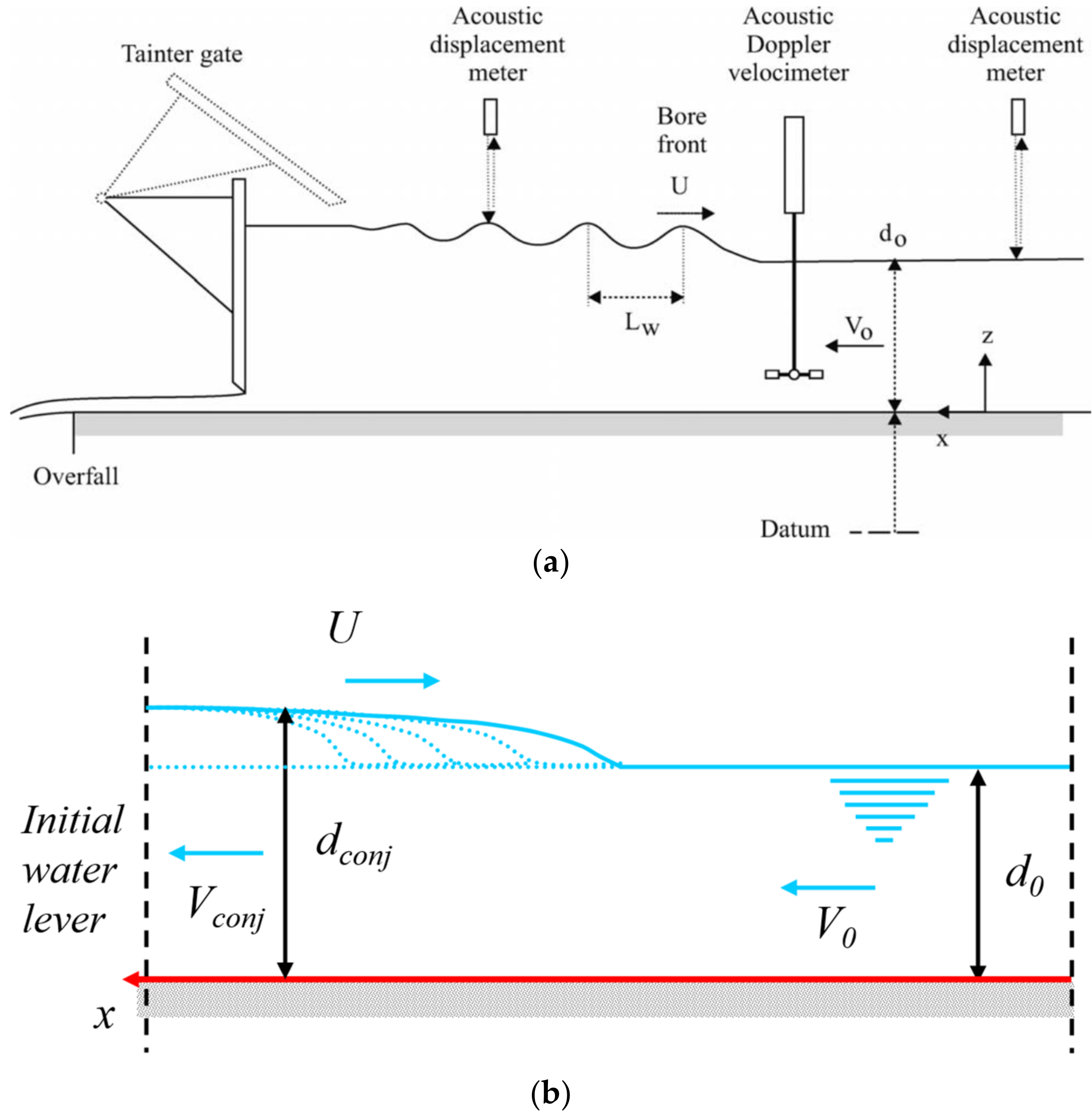
Figure 2.
Dimensionless velocity distribution in the steady flow. Time-averaged velocity Vx/V*. Comparison between ADV data, law of the wall, and Osterlund [39] (redrawn from [16]).

Figure 3.
Flow chart for calculating the Kolmogorov complexity spectrum.

Figure 4.
Undular surge, Run 60-7. Dimensionless instantaneous water depth d/d0 and velocity components Vx/V* and Vy/V* at (a) z/d0 = 0.060; (b) at z/d0 = 0.793 (redrawn from [17]).
Figure 4.
Undular surge, Run 60-7. Dimensionless instantaneous water depth d/d0 and velocity components Vx/V* and Vy/V* at (a) z/d0 = 0.060; (b) at z/d0 = 0.793 (redrawn from [17]).
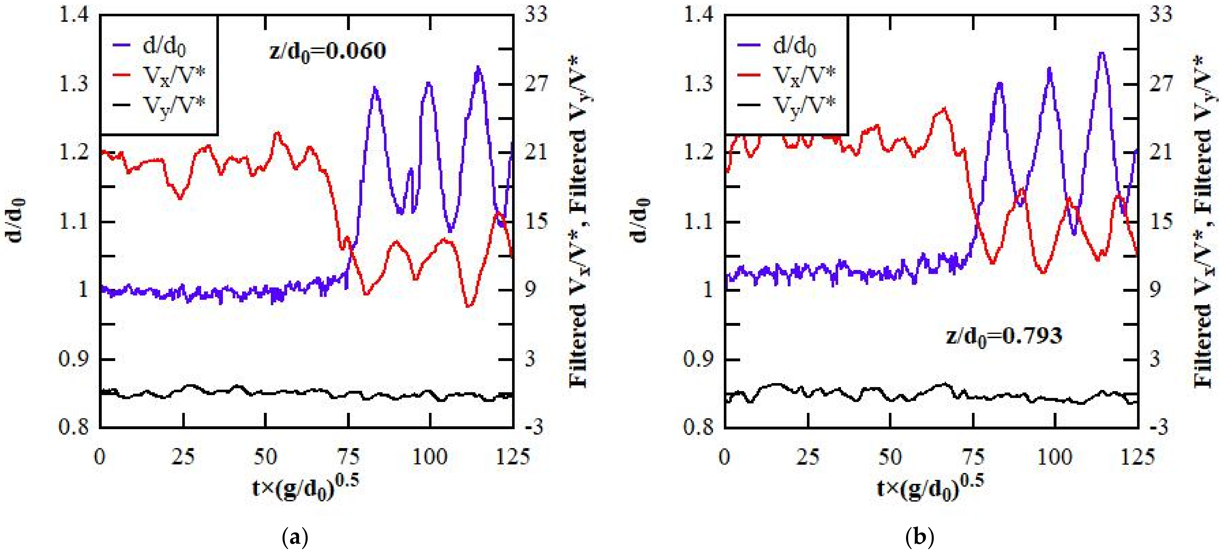
Figure 5.
Breaking surge, Run 60-6. Dimensionless instantaneous water depth d/d0 and velocity components Vx/V* and Vy/V* (a) at z/d0 = 0.060 (left); (b) at z/d0 = 0.738 (redrawn from [17]).
Figure 5.
Breaking surge, Run 60-6. Dimensionless instantaneous water depth d/d0 and velocity components Vx/V* and Vy/V* (a) at z/d0 = 0.060 (left); (b) at z/d0 = 0.738 (redrawn from [17]).
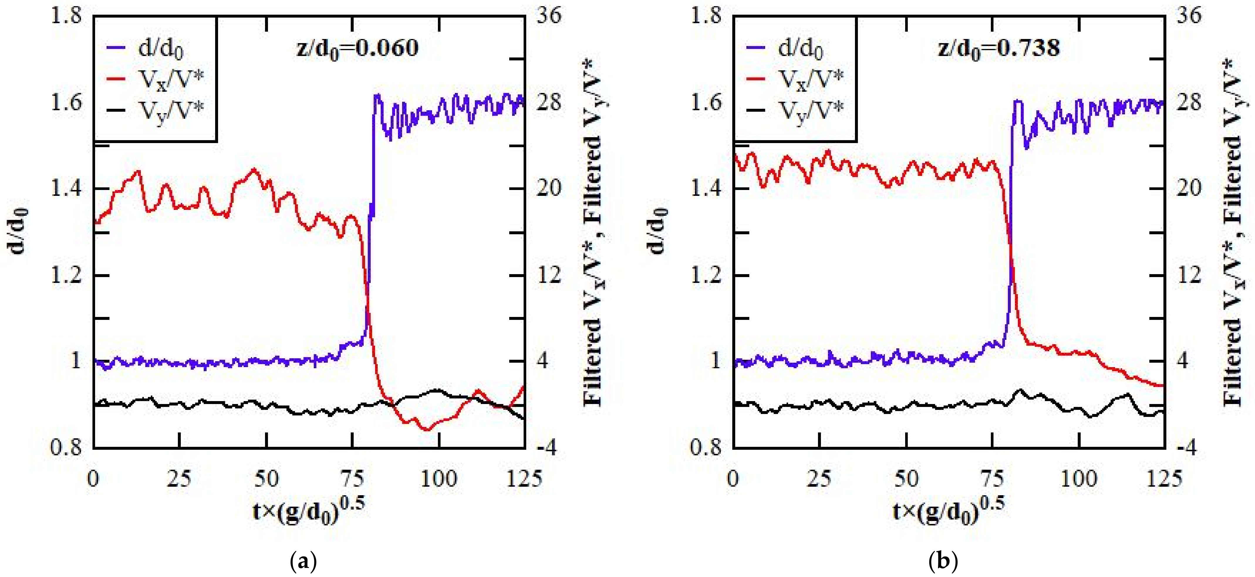
Figure 6.
Undular surge, Run 60-7. Dimensionless normal Reynolds stresses (a) Vx2/V*2; (b) Vy2/V*2.

Figure 7.
Breaking surge, Run 60-6. Dimensionless normal Reynolds stresses (a) Vx2/V*2; (b) Vy2/V*2.
Figure 7.
Breaking surge, Run 60-6. Dimensionless normal Reynolds stresses (a) Vx2/V*2; (b) Vy2/V*2.
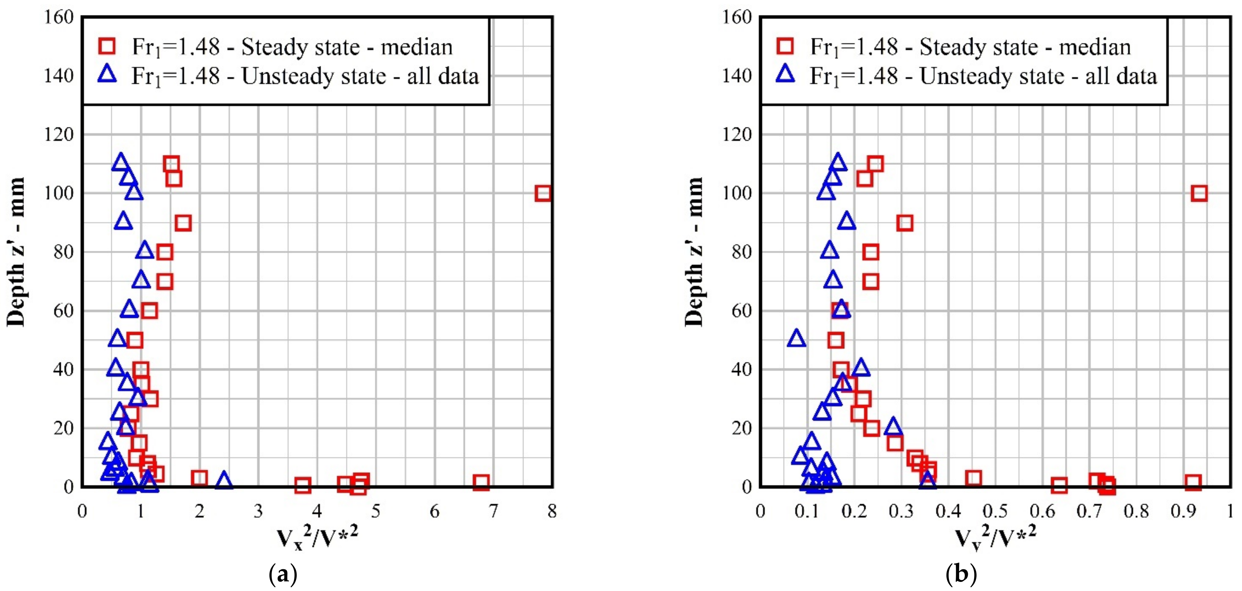
Figure 8.
Undular surge, Run 60-7. Kolmogorov complexity vs. vertical elevation z′ for (a) Vx; (b) Vy.
Figure 8.
Undular surge, Run 60-7. Kolmogorov complexity vs. vertical elevation z′ for (a) Vx; (b) Vy.

Figure 9.
Breaking surge, Run 60-6. Kolmogorov complexity vs. vertical elevation z′ for (a) Vx; (b) Vy.
Figure 9.
Breaking surge, Run 60-6. Kolmogorov complexity vs. vertical elevation z′ for (a) Vx; (b) Vy.
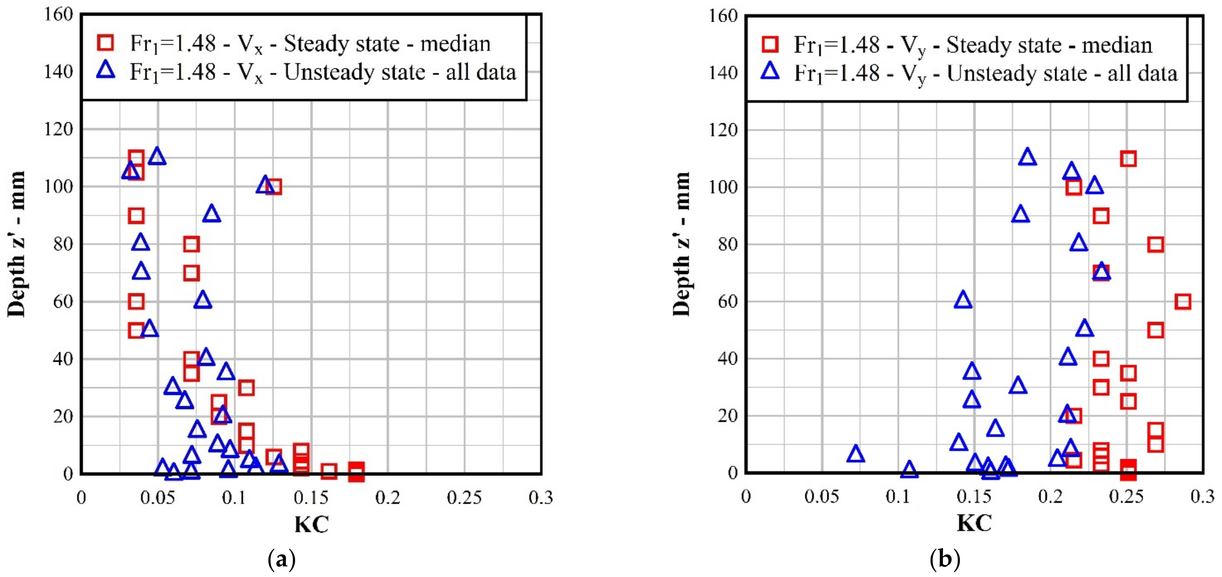
Figure 10.
Undular surge, Run 60-7, and breaking surge Run 60-6. Kolmogorov complexity spectra for Vx at z′ = 0.00 mm and 100 mm.
Figure 10.
Undular surge, Run 60-7, and breaking surge Run 60-6. Kolmogorov complexity spectra for Vx at z′ = 0.00 mm and 100 mm.
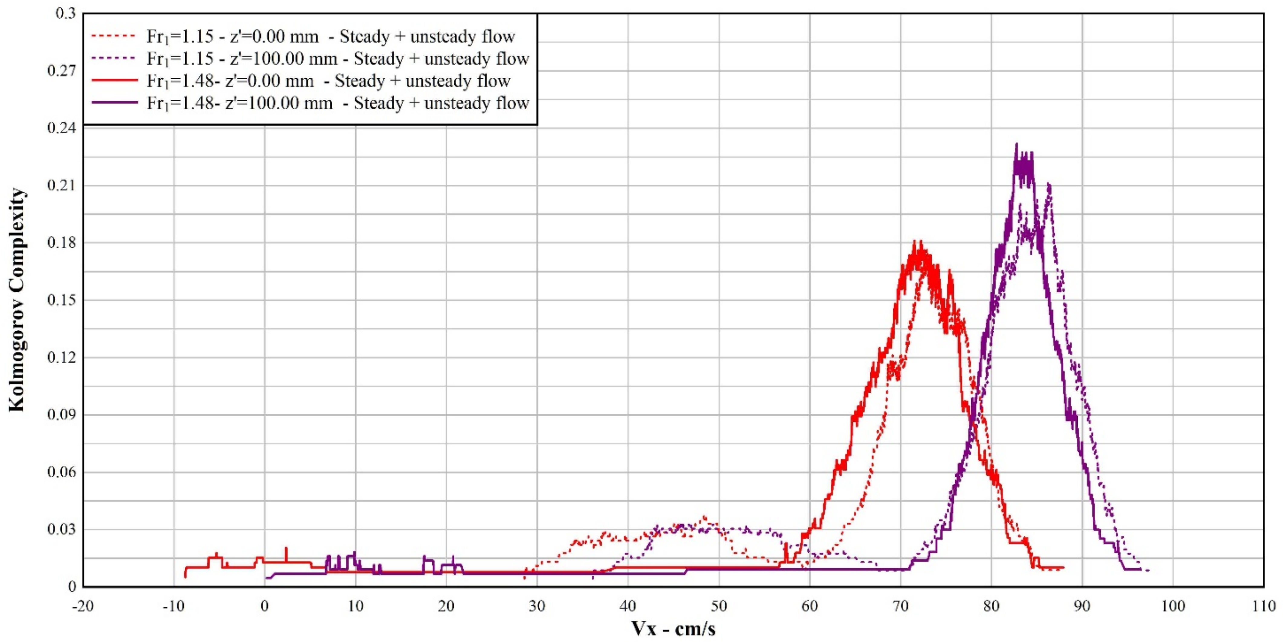
Figure 11.
Undular surge, Run 60-7 and breaking surge Run 60-6. Kolmogorov complexity spectra for Vy at z′ = 0.00 mm and 100 mm.
Figure 11.
Undular surge, Run 60-7 and breaking surge Run 60-6. Kolmogorov complexity spectra for Vy at z′ = 0.00 mm and 100 mm.

Table 1.
Experimental flow conditions.
| Run | Q—m3/s | d0—m | hg—m | Type | U—m/s | dconj—m | Fr1 | Remarks |
|---|---|---|---|---|---|---|---|---|
| 60-6 | 0.060 | 0.1429 | 0.005 | Breaking | 0.918 | 0.237 | 1.484 | ADV measurements |
| 60-7 | 0.060 | 0.1427 | 0.100 | Undular | 0.519 | 0.171 | 1.149 | ADV measurements |
Publisher’s Note: MDPI stays neutral with regard to jurisdictional claims in published maps and institutional affiliations. |
© 2022 by the authors. Licensee MDPI, Basel, Switzerland. This article is an open access article distributed under the terms and conditions of the Creative Commons Attribution (CC BY) license (https://creativecommons.org/licenses/by/4.0/).
Share and Cite
MDPI and ACS Style
Gualtieri, C.; Mihailović, A.; Mihailović, D. An Application of Kolmogorov Complexity and Its Spectrum to Positive Surges. Fluids 2022, 7, 162. https://doi.org/10.3390/fluids7050162
AMA Style
Gualtieri C, Mihailović A, Mihailović D. An Application of Kolmogorov Complexity and Its Spectrum to Positive Surges. Fluids. 2022; 7(5):162. https://doi.org/10.3390/fluids7050162
Chicago/Turabian StyleGualtieri, Carlo, Anja Mihailović, and Dragutin Mihailović. 2022. "An Application of Kolmogorov Complexity and Its Spectrum to Positive Surges" Fluids 7, no. 5: 162. https://doi.org/10.3390/fluids7050162