Numerical Simulation of High-Density Ratio Bubble Motion with interIsoFoam

Abstract

The breeding blanket is one of the fundamental components of a nuclear fusion reactor and is responsible for the fuel production, generating tritium through neutronic capture reaction between lithium and neutrons. Lithium is a liquid PbLi alloy and the helium formed as reaction by-product can coalesce into bubbles, generating a two-phase mixture with a high-density ratio (${\eta }_{\rho }\sim {\mathcal{O}}^5$). These bubbles can accumulate and stagnate within the blanket channels with potentially harmful consequences. In this work, the interIsoFoam solver of OpenFOAM v2012 is used to simulate bubble motion for a two-phase mixture representative of the He-PbLi system to test its potential for future developments in the field of fusion. In a first phase, several traditional benchmarks were carried out, both 2D and 3D, and considering the two variants of the VOF method implemented in the solver, isoAdvector and plicRDF. Subsequently, He bubbles of different diameters rising in liquid PbLi (${\eta }_{\rho }=1.2\times {10}^5$) were analysed to investigate different regimes. For a Eötvös number (Eo) greater than 10, it was possible to recreate the axisymmetric, skirted, oscillatory regimes and the peripheral and central breakup regimes. For Eo < 10, non-physical deformations of the interface are observed, probably generated by spurious velocities that have a greater impact on the solution for very small bubbles and rising velocities.

1. Introduction

The breeding blanket (BB) is a quite complex system of a nuclear fusion reactor which primary function is the production of tritium ($\mathrm{T}={}^3\mathrm{H}$), one of the reagents for the nuclear reaction powering the device. Indeed, tritium does not exist naturally in any meaningful quantity for industrial applications, since it is characterized by a relatively short half-life (12.3 years), and has to be breed from lithium (Li) according to the neutron capture reaction [1]:

$${}^6\mathrm{Li}+\mathrm{n}\to {}^4\mathrm{He}+\mathrm{T}$$

(1)

In several BB concepts lithium is employed in a liquid PbLi alloy and the helium (He) formed as reaction by-product, given its essentially insolubility in a liquid metal and its high production rate, can forms bubbles. These bubbles might impact the blanket performance, affecting the heat transfer and tritium migration mechanisms, even causing cavitation or channels blockage, therefore their transport should be considered in the breeding blanket design [2,3].

In general, there are several approaches to simulate multi-phase flows [4], among them implicit interface capturing methods, or volume of fluid (VOF) [5], and the level-set methods [6], have recently attracted a lot of attention as a valid options to simulate flows in which there is an extensive variation of the topology of the phasic interface. As stated in [7], there are at least four issues related to interface capturing methodologies: accurate interface representation and advection, mass conservation, spurious velocities and handling large density ratios.

In the VOF method, the interface location is calculated implicitly through a fraction or indicator function which, assuming the discrete values 0 or 1 in each node of the computational grid, maps the two phases over the volume. The discontinuity of this function causes a difficulty in its advection, that results in an excessive diffusion of the interface. Attempts to get around this problem are divided into two classes of methodologies: geometric and algebraic methods.

The geometric methods explicitly reconstruct a sub-cell representation of the interface using an assumed functional form and then advect it in a Lagrangian sense to accurately compute volume fluxes. In this way, the numerical diffusion of the interface is definitively avoided but there are still some unresolved problems, such as the difficulty of implementation in higher dimensions and the increase in computational expense [7].

The algebraic methods completely eliminate the reconstruction procedure and instead use algebraic manipulations such as high-resolution or compressive differentiation schemes. This greatly simplifies the algorithm, reducing the computational cost of the procedure, but causes a reduction in accuracy. The result is that the interface calculated by an algebraic method may be spread over two or three cells rather than being precisely known [7]. Aside from accurate advection of the fraction function, difficulties arise in estimating the curvature of the interface due to the discontinuous nature of the volume fraction field and, in this regard, several alternatives, including smoothing of the volume fraction field and the construction of the height function [8], have been suggested.

The level-set methods, instead, use a continuous “level-set function” which assumes the value zero at the interface which is implicitly manipulated [6] and, therefore, they are not affected by the problem described above and offer a more accurate representation of the interfacial quantities such as interfacial normal and curvature [7]. Numerical methods which are based on the VOF intrinsically conserve mass while those based on the level-set do not embed mass conservation in their formulation. Consequently, highly curved or poorly resolved regions of the flow are typically susceptible to such mass loss. Significant improvements have been made in this regard through the development of techniques such as the use of marker particle interface advection [9], VOF coupling with level-set methods [10] and an augmented gradient layer-set method [11].

Almost all implicit interface capture methods are susceptible to non-physical velocities generated at the interface, called spurious velocities or currents, which are generated by an inaccurate evaluation of the curvature of the interface or by the lack of an accurate force balance between pressure and surface tension [12]. Although a spurious velocity generation is not a major problem for inertia-dominated flows, it raises serious concerns in the calculation of capillary flows, which generally characterize small liquid structures in hydrodynamic flows that involve atomization. Several strategies have been studied to mitigate the problem and a large collection can be found in Ref. [7].

It is known that the simulation of flows with high density ratios is a difficult task. Inconsistencies in the formulation of continuity and momentum equations can cause the prediction of non-physical phenomena including, but not limited to, the artificial deformation of the interface [7,13], a critical aspect for a He-PbLi mixture, in which ${\eta }_{\rho }\sim {\mathcal{O}}^5$.

In this work, the dynamic of a rising helium bubble in PbLi at different flow regimes is numerically analysed using the OpenFOAM interIsoFoam solver. The solver was first validated through various benchmarks and its performance with respect to a wide range of density ratio between the phases have been investigated. Overall, interIsoFoam is able to reliably simulate the bubble motion in a two-phase flow with high-density ratio and it will be used as a foundation for developing a multi-phase magnetohydrodynamics (MHD) solver to investigate the bubble motion in a liquid metal subjected to the magnetic field present in a magnetic confinement fusion reactor. Indeed, the movement of PbLi, being an electrically conductive liquid, is influenced by the magnetic field through the onset of MHD effects. These change the balance of forces in the fluid and at the interface between the fluid and gas phase, modifying the dynamics of the bubble [14,15,16].

The possibility of analysing these effects through an MHD solver capable of simulating mixtures of a liquid metal and a gas is, indeed, very important both for the design of the breeding blanket [2,3] and for the plasma-facing components, in which advanced solutions may foresee the employment of liquid metal films, jet curtains and other solutions to protect the solid substrate below from the thermal and radiative load coming from the plasma [17,18,19].

2. Code Description and Methods

The interIsoFoam solver is a recent variant of the standard algebraic VOF interFoam solver [20], originally developed by Weller [21], introduced starting with OpenFOAM v1706 for two incompressible, isothermal, immiscible fluids. It employs the geometric VOF method, named isoAdvector, developed by Roenby et al. [22,23]. More recently, the solver was integrated with a novel interface reconstruction method, introduced by Scheufler et al. [24], where the construction employs a reconstructed distance function (RDF).

Without claiming to be exhaustive, the VOF methodology implemented in interFoam is briefly presented below, with the solutions adopted in the three possible schemes for the interface advection method in interIsoFoam. For a more detailed discussion, see Refs. [7,22,24].

The VOF method is a variant of the more general Eulerian-Eulerian multi-phase model that employs a single momentum equation for phases, employing the fraction function

$$F(\mathit{x},t)=\left\{\begin{array}{c}1\mathrm{for}\mathit{x}\in {\alpha }_1\mathrm{at}\mathrm{time}t\hfill \\ 0\mathrm{for}\mathit{x}\in {\alpha }_2\mathrm{at}\mathrm{time}t\hfill \end{array}\right.$$

(2)

which assumes the unitary value in the points in which phase 1, ${\alpha }_1$, is present at time t, and the zero value in the points in which phase 2, ${\alpha }_2$, is present at time t. From Equation (2), we obtain the volume fraction function $r_{\alpha }$ by integrating the fraction function over the control volume (CV)

$$r_{\alpha }({\mathit{x}}_i,t)={\displaystyle \frac{1}{{\mathsf{\Omega }}_{CV}}}{\int }_{CV}^{}FdV\in [0;1]$$

(3)

where ${\mathsf{\Omega }}_{CV}$ is the CV volume.

The integrated momentum equation over the generic CV becomes [7]

$${\int }_{CV}^{}\left\{\rho \left[\frac{\partial \mathit{u}}{\partial t}+\left(\mathit{u}·\nabla \right)\mathit{u}\right]dV\right\}={\int }_{CV}^{}\left[-\nabla p+\rho \nu {\nabla }^2\mathit{u}+\rho \mathit{g}+\gamma \kappa \nabla r_{\alpha }\right]dV$$

(4)

where $\mathit{u}$ is the velocity, p the pressure, $\mathit{g}$ the gravitational acceleration, $\rho$ the density, $\nu$ the kinematic viscosity, $\gamma$ is the surface tension and $\kappa$ is the interface curvature. The surface tension term (right-hand side last term) is written as a volumetric force following the continuum surface force (CSF) model of Brackbill et al. [25]. The interface curvature is obtained from the volume fraction by the relation

$$\kappa =\nabla ·\left({\displaystyle \frac{\nabla r_{\alpha }}{|\nabla r_{\alpha }|}}\right)$$

(5)

and the density and kinematic viscosity takes the discontinuous form

$$\varphi ={\varphi }_{1}F+{\varphi }_2(1-F)$$

(6)

where ${\varphi }_1$ and ${\varphi }_2$ are constant in each respective phase. To mathematically close the system, a transport equation for the fraction volume must be added to Equation (4) which, integrated above the generic CV, takes the form

$${\int }_{CV}^{}\left[\frac{\partial r_{\alpha }}{\partial t}+\nabla ·\left(\mathit{u}{r}_{\alpha }\right)\right]=0$$

(7)

Equation (7) is the fundamental equation of the VOF method, whose resolution must preserve the sharpness of the interface. Regardless of the numerical scheme used to solve Equation (7), interFoam and interIsoFoam solve the governing equations in a segregated way through the PIMPLE algorithm for pressure-velocity coupling. This method is a hybrid version between the PISO algorithm and the SIMPLE algorithm, which guarantees better stability for problems that involves very large time-steps and pseudo-transient simulation, carrying out others iterative cycles outside the PISO ones.

In interFoam, the sharpness of the interface is obtained by algebraically modifying the advection term of Equation (7), dividing it into two parts: one that is always different from zero and the other that has a non-zero value only at the interface, which it is to say in the CVs in which $0<r_{\alpha }<1$, through a limiter implemented in the MULES solver [20]. In this way, in all CVs containing one of the two phases, the Equation (7) is discretized with a certain numerical scheme and in the CVs containing the interface the order of the scheme is increased considering this additional term $\nabla ·\left(r_{\alpha }(1-r_{\aleph }\mathit{u})\right)$, called interfacial compression term. In this way, the numerical diffusion is reduced and the computational cost of the scheme is increased only at the interface. For a detailed description of the algorithm, see the Ref. [7]. The interFoam solver has been extensively validated but, under certain conditions, fails to keep the interface sharp enough and the heuristic nature of the interface compression term can lead to an inaccurate advection of the interface [22,26].

The isoAdvector method geometrically reconstructs the interface through a sub-grid reconstruction-step and then advects the interface within the time-step (the advection-step). The reconstruction-step is based on the construction of a planar isosurface, called isoface, inside the CVs located on the interface, i.e., having $0<r_{\alpha }<1$. To do this, the $r_{\alpha }$ values stored in the centre of the CV are interpolated at its vertices and, from these values, the isoface is calculated at a value of $r_{\alpha }$, specific for the single CV, so that the two generated sub-volumes are proportional to the volume fraction in the specific CV. Then, the isoface motion is estimated within the time-step, in the advance-step, using the velocity data of the surrounding cells and therefore, in practice, evaluating the motion in a sub-time step. The intersection of the isoface with the faces of the CV generates the face-interface intersection line which is used to determine the volume of ${\alpha }_1$ transported through the face from which the new distribution of $r_{\alpha }$ in the domain is derived. For a detailed discussion, see the paper by Roenby et al. [22].

A problem of the isoAdvector reconstruction technique is related to the local interface orientation, which converges slowly in the structured meshes and does not converge at all in the unstructured ones [24]. A solution to this problem is presented by Scheufler and Roenby [24], who employed an iterative method using a RDF to estimate the position and orientation of the interface from the raw volume fraction data. They presented two versions of the algorithm. In the first variant, called iso-RDF, the values of the interface centre position and its normal provided by the isoAdvector algorithm are used as an initial guess for an iterative RDF-based method that is repeated until a certain tolerance on the change in interface orientation is reached. The RDF is calculated from the shortest distance from the cell centre to the plane.

In the second variant, called plic-RDF, the isoface calculation is replaced with a more traditional gradient calculation of $r_{\alpha }$ in the estimations of the interface normal, through the PLIC algorithm. The novelty is the usage of interface normal information from the previous time-step, improving the normal value initial guess, and the use of a residual convergence criteria for normal calculation, based on the local evaluation of the curvature interface. In this way, in areas where the curvature is under-resolved and where information on its orientation is missing, the algorithm limits the number of iterations that could not compensate for the lack of this information, resulting in a waste of computational resources [24].

The RDF method, which is combined with the isoAdvector advection-step, has shown a second order convergence with mesh refinement for both 2D and 3D cases, both for structured and unstructured meshes, in the calculation of the interface position and its orientation. For a detailed discussion, please refer to the original work in Ref. [24].

3. Results

3.1. interIsoFoam Validation

3.1.1. 2D Stationary Drop

The first benchmark proposed is the verification of the stationary solution for a circular drop with diameter d under zero gravity. In this scenario, no velocity field must be present, the interface must remain circular and the pressure jump must exactly balance the surface tension. Indeed, from Equation (4) we have the Laplace relation

$$\begin{array}{cc}\hfill & \Delta p=\gamma \kappa \hfill \end{array}$$

(8)

$$\begin{array}{cc}\hfill & \kappa ={\displaystyle \frac{2}{d}}\hfill \end{array}$$

(9)

As mentioned in the introduction, during the numerical resolution, a velocity field can be generated (spurious velocity) due to the discretization error that is generated between the imbalance of the pressure and the surface force, essentially due to an inappropriate numerical scheme for the balance and/or an inaccurate computation of the curvature. The resolution of a static drop has been widely used as a test case to evaluate the impact of these two elements on resolution [10,26,27,28]. In this work this test will be performed with a unit density ratio (${\eta }_{\rho }={\rho }_{{\alpha }_1}/{\rho }_{{\alpha }_2}$) and then repeated for ${\eta }_{\rho }=1000$.

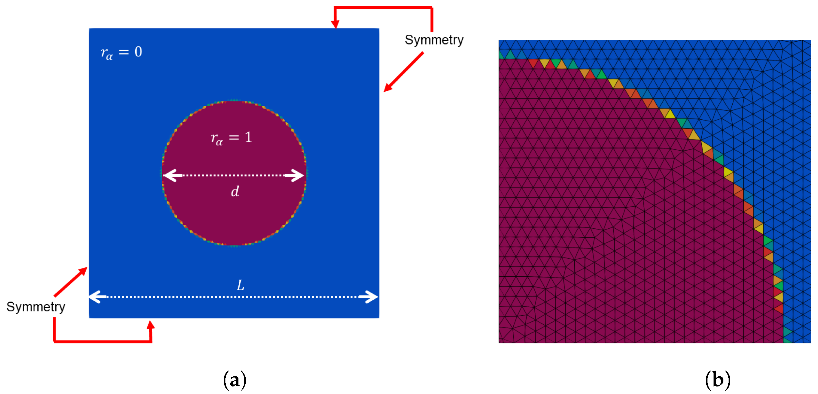
Figure 1a shows the computational domain, which is a 2D square with side $L=2d$ with the drop positioned in the centre (initial condition, IC), and the boundary conditions (BCs). The thickness in the non-considered direction, in all the 2D models analysed below, has a value equal to the largest dimension of the mesh element employed case-by-case. No subdivision is applied in that direction.

The surface tension and the kinematic viscosity of both the phases are unitary ($\gamma =1\mathrm{N}{\mathrm{m}}^{-1}$, ${\nu }_{{\alpha }_1}={\nu }_{{\alpha }_2}=1{\mathrm{m}}^2{\mathrm{s}}^{-1}$), while ${\rho }_{{\alpha }_1}={\rho }_{{\alpha }_2}=1\times {10}^4\mathrm{kg}{\mathrm{m}}^{-3}$ for the ${\eta }_{\rho }=1$ case and ${\rho }_{{\alpha }_1}=1000\mathrm{kg}{\mathrm{m}}^{-3}$ and ${\rho }_{{\alpha }_2}=1\mathrm{kg}{\mathrm{m}}^{-3}$ for the ${\eta }_{\rho }=1000$ case. As shown in Figure 1a, the symmetry BC has been set on the sides of the square, while the empty BC, which is the standard condition in OpenFOAM for boundaries positioned in the non-considered direction of a 2D model, has been used on the faces. Through the utility setAlphaField, we have imposed $r_{\alpha }=1$ in the CVs inside the circumference and $r_{\alpha }=0$ in the external CVs, initializing the drop.

The Crank-Nicolson second order scheme with a blending factor equal to 0.9 has been employed for the temporal discretization, the Gauss pointCellsLeastSquares scheme for the gradient discretization, the limitedLinearV scheme with a blending factor equal to 1 for the velocity advection term discretization and the vanLeer scheme has been employed for the volume fraction advection discretization. Three PISO cycles and three external PIMPLE cycles have been performed, using the solver smoothSolver with the symGaussSeidel smoother for the velocity resolution and the GAMG solver with the DIC smoother for the pressure. The isoAdvector method with 2 plic-RDF iterations in the reconstruction-step of the interface has been used. As indicated in [24], the maximum CFL number was imposed equal to 0.2 to guarantee a second order convergence for the interface advection step.

The mesh used, shown in Figure 1b, is triangular and unstructured. To evaluate the influence of the mesh size on the results, a mesh sensitivity was carried out considering three different grid sizes (h), which corresponds to the maximum length of the mesh element, whose data are collected in

Table 1. Mesh data and results for the mesh sensitivity study and for the ${\eta }_{\rho }=1000$ case, simulated with the M2 mesh.

	Grid Size h (m)	Number of Elements	${\mathit{L}}_1\left(\mathit{u}\right)$	$\mathit{E}(\mathbf{\Delta }\mathit{p})$
M1	0.04	1400	2.68 × 10−3	0.125
M2	0.02	5678	1.84 × 10−3	0.068
M3	0.01	22,902	1.30 × 10−3	0.146
${\eta }_{\rho }=1000$	0.02	5678	4.1 × 10−1	0.075

together with the results of the study. The simulations were carried out on the Sigmar server at the DIAEE Department of Sapienza University of Rome, which uses Intel Xeon E5-2690 v3 2.60 GHz processors, like all the simulations presented in this work. A number of parallel processors equal to 1 (serial), 4 and 8 were used for, respectively, the meshes M1, M2 and M3 (Table 1), with a computational time to ensure that all the residuals are below 1 × 10⁻⁷ (about 125 s of transient) in the range $1÷4.5$ h.

The parameters used for the evaluation are the error on the pressure jump $E(\Delta p)$ and the $L_1\left(\mathit{u}\right)$ error norm to quantify the error on the velocity:

$$\begin{array}{cc}\hfill & E(\Delta p)={\displaystyle \frac{\left|p_{in}-p_{out}-2\gamma /d\right|}{2\gamma /d}}\hfill \end{array}$$

(10)

$$\begin{array}{cc}\hfill & L_1\left(\mathit{u}\right)={\displaystyle \frac{1}{\mathsf{\Omega }}}{\int }_{\mathsf{\Omega }}^{}{\displaystyle \frac{\sqrt{{\left(\mathit{u}·\mathit{u}\right)}^2}\mu }{\gamma }}dV\hfill \end{array}$$

(11)

where $p_{in}$ and $p_{in}$ are, respectively, the pressure inside the drop and the pressure outside the drop and $\mathsf{\Omega }$ is the total model volume. The quantities $p_{in}$ and $p_{out}$ were calculated from the volumetric average of the pressure considering, respectively, the isovolume $0.5\le r_{\alpha }\le 1$ and $0\le r_{\alpha }\le 0.5$.

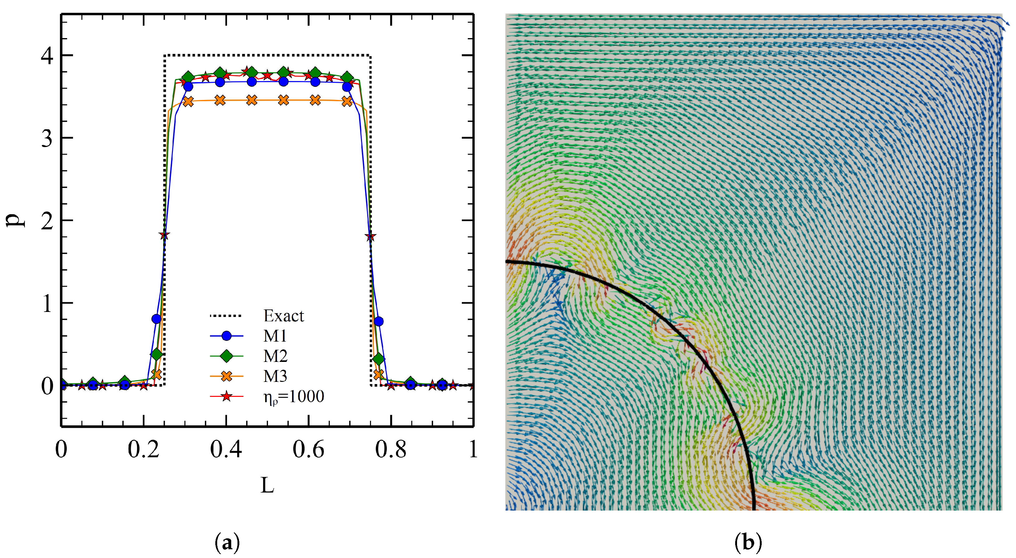
As shown in Table 1 and in Figure 2a, for all the tested meshes and regardless of ${\eta }_{\rho }$, the pressure jump is underestimated by ∼10% regardless of the mesh used, as already seen by Deshpande et al. [7] for the interFoam solver. This discrepancy is probably due to the low number of iterations (2) performed on the RDF function, indeed in Ref. [26] the same test with 5 iterations has eliminated this discrepancy. Regarding the spurious velocities, from Table 1 and Figure 2b we can see how they are generated at the interface, where they remain quite low for ${\eta }_{\rho }=1$ and decrease as the mesh resolution increases, but increase by about two orders of magnitude passing to ${\eta }_{\rho }=1000$.

3.1.2. 2D Rising Bubble

This test was solved by Hysing et al. [29], comparing the numerical results of three different codes (TP2D, FreeLIFE and MooNMD). The relevant physical parameters that describes completely a rising bubble are the Eötvös or Bond number

$$Eo={\displaystyle \frac{g{L}_c{\rho }_{{\alpha }_1}}{\gamma }}$$

(12)

which measures the importance of the gravitational forces compared to the surface tension ones, where the characteristic length is the bubble diameter ($L_c=d$), the Galilei number

$$\begin{array}{cc}\hfill & Ga={\displaystyle \frac{\rho U_g{L}_c}{{\mu }_{{\alpha }_1}}}\hfill \end{array}$$

(13)

$$\begin{array}{cc}\hfill & U_g=\sqrt{g{L}_c}\hfill \end{array}$$

(14)

which is similar to the Reynolds number but, instead of using the bubble terminal velocity, uses the gravitational velocity $U_g$ and the density (${\eta }_{\rho }$) and viscosity (${\eta }_{\mu }={\mu }_{{\alpha }_1}/{\mu }_{{\alpha }_2}$) ratio. An additional parameter is the Morton number which depends only from the surrounding fluid

$$Mo={\displaystyle \frac{g{\mu }_{{\alpha }_1}^4}{{\rho }_{{\alpha }_1}{\gamma }^3}}$$

(15)

Two scenarios are proposed in Ref. [29]: the C1 scenario, where there are a low density ratio and Eötvös number and the bubble undergoes moderate shape deformation, and the C2 scenario in which these two parameters increase and the bubble surface is warped more significantly, generating filaments that, eventually, can break off. The data of the cases are collected in

Table 2. Parameters for the 2D rising bubble test.

	${\mathit{\eta }}_{\mathit{\rho }}$	${\mathit{\eta }}_{\mathit{\mu }}$	g (m s${}^{-2}$)	$\mathit{\gamma }$ (N m${}^{-1}$)	Eo	Ga
C1	10	10	0.98	24.5	10	35
C2	1000	100	0.98	1.96	125	35

.

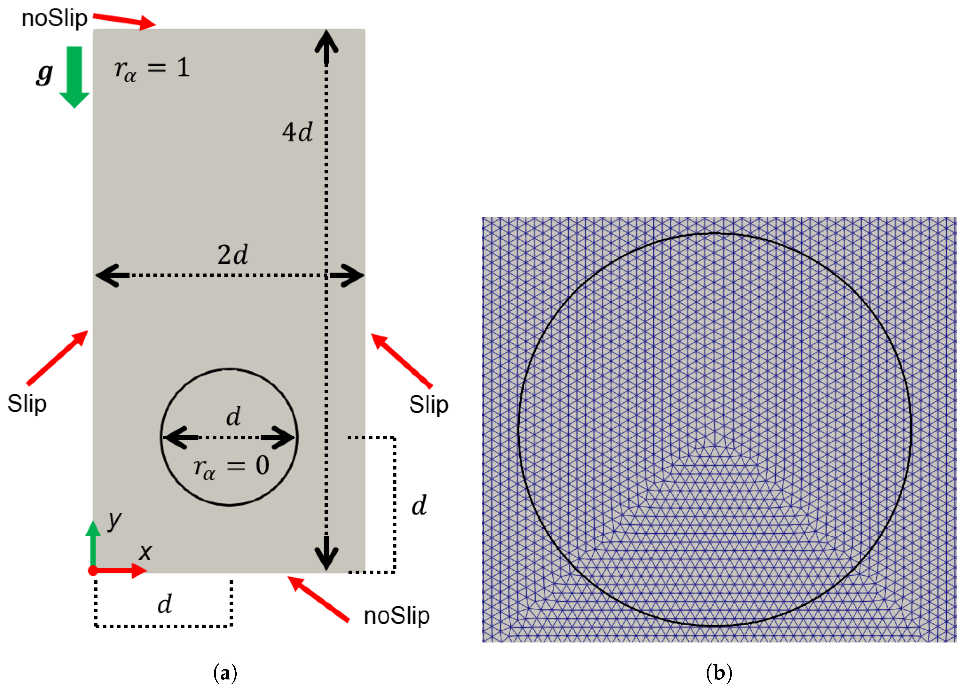
The computational domain is composed of a rectangle whose sides in x and y-direction are, respectively, equal to $2d$ and $4d$, where d is the bubble diameter. The bubble is centred in the lower half of the rectangle, as shown in Figure 3a. In this figure, the imposed BCs for the velocity are also shown, that is the noSlip condition for the bottom and top boundaries and the slip condition, which imposes a zero shear stress, on the vertical boundaries. For pressure, the zeroGradient BC has been employed, whereas for the faces normal to the non-considered direction the empty condition has been employed. The light phase constituting the bubble (${\alpha }_2$) is initialized as described in Section 3.1.1, as well as the numerical set up, with the only difference in the value of the gravity acceleration which, in this case, has a finite value (Table 2). The mesh used is triangular and unstructured, shown in Figure 3b.

The parameters used as benchmarks are [29]: the vertical position (y-direction) of the bubble centroid ($y_c$), the bubble rising velocity, which corresponds to the y-components of the velocity of the centroid ($u_c$), and the bubble circularity $\xi$, which measures how far the shape of the bubble differs from the circular one, being $\xi =1$ for the circular shape, at $t=0$, and decreasing progressively as the bubble is deformed. The relations computed in the code in order to obtain these parameters are are the follows:

$$\begin{array}{cc}\hfill & y_c={\displaystyle \frac{1}{{\mathsf{\Omega }}_{{\alpha }_2}}}{\int }_{\mathsf{\Omega }}^{}(1-r_{\alpha })ydV\hfill \end{array}$$

(16)

$$\begin{array}{cc}\hfill & {\mathsf{\Omega }}_{{\alpha }_2}={\int }_{\mathsf{\Omega }}^{}(1-r_{\alpha })dV\hfill \end{array}$$

(17)

where ${\mathsf{\Omega }}_{{\alpha }_2}$ is the bubble volume,

$$u_c={\displaystyle \frac{1}{{\mathsf{\Omega }}_{{\alpha }_2}}}{\int }_{\mathsf{\Omega }}^{}(1-r_{\alpha })u_{y}dV$$

(18)

and

$$\xi ={\displaystyle \frac{\sqrt{{\displaystyle \frac{{\mathsf{\Omega }}_{{\alpha }_2}}{\pi \Delta z}}}}{{\displaystyle \frac{A_{{\alpha }_2}}{2\pi \Delta z}}}}$$

(19)

where $A_{{\alpha }_2}$ ia the bubble surface, computed considering the triangulated isosurface at $r_{\alpha }=0.5$, $\Delta z$ is the cell size in the non-considered direction. In particular, the minimum value of the circularity (${\xi }_{min}$) during the simulation has been considered, as well as the time at which the minimum occurs (${t|}_{\xi ={\xi }_{min}}$). Please note that the total simulation time has been chosen as 3 s. Regarding the rising velocity, the maximum value ($u_{c,max}$), the instant of its occurrence (${t|}_{u_c=u_{c,max}}$) and, finally, the position of the centroid at 3 s have been considered.

For the C1 scenario, the code has been tested with both the reconstruction methods implemented in isoAdvector: the plicRDF reconstruction method (2 iterations), also used in Section 3.1.1, and the original one proposed by Roenby et al. [22] (Section 2), here called isoAlpha. For this case, a mesh sensitivity study was carried out considering four meshes, which data are collected in

Table 3. Mesh data for 2D rising bubble mesh sensitivity study.

	Grid Size h (m)	Number of Elements
M1	0.01250	29,344
M2	0.00833	66,854
M3	0.00625	116,142
M4	0.00500	184,398

, while the results are shown in

Table 4. Mesh sensitivity study results for 2D rising bubble for both isoAlpha and plicRDF methods.

	isoAlpha			plicRDF
	${\mathit{\xi }}_{\mathit{min}}$	${\mathit{u}}_{\mathit{c},\mathit{max}}$ (m s${}^{-1}$)	${\mathit{y}}_{\mathit{c}}$ (t = 3 s)	${\mathit{\xi }}_{\mathit{min}}$	${\mathit{u}}_{\mathit{c},\mathit{max}}$ (m s${}^{-1}$)	${\mathit{y}}_{\mathit{c}}$ (t = 3 s)
M1	0.8939	0.2414	1.0831	0.8945	0.2413	1.0832
M2	0.8947	0.2409	1.0833	0.8946	0.2408	1.0834
M3	0.8952	0.2415	1.0839	0.8953	0.2413	1.0840
M4	0.8952	0.2417	1.0840	0.8955	0.2414	1.0841

. A number of parallel processors equal to 1 (serial) and 9 were used for, respectively, the meshes M1 and M4 (Table 3), with a computational time to terminate the transient (3 s) equal to, respectively, about 1.5 and 3 h. For both the solver variants, the results for meshes M2, M3 and M4 differ by less than 1%. The only parameter on which the mesh resolution has a relative higher impact is the circularity, which for the isoAlpha variant has an average variation of ≃1.8%, while for the plicRDF solver is equal to ≃0.7%.

For the benchmark, the results provided by Hysing et al. [29] for the TP2D code and by Balcázar et al. [10], that developed an hybrid VOF/level-set code, were considered. The results, provided for the M3 mesh, are collected in

Table 5. Benchmark results for C1 case (M3 mesh) for both isoAlpha and pliRFD method compared with Refs. [10,29].

	${\mathit{\xi }}_{\mathit{min}}$	${\mathit{t}|}_{\mathit{\xi }={\mathit{\xi }}_{\mathit{min}}}$	${\mathit{u}}_{\mathit{c},\mathit{max}}$ (m s${}^{-1}$)	${\mathit{t}|}_{{\mathit{u}}_{\mathit{c}}={\mathit{u}}_{\mathit{c},\mathit{max}}}$	${\mathit{y}}_{\mathit{c}}$ (t = 3 s)
isoAlpha	0.8952	1.8900	0.2415	0.9260	1.0839
plicRDF	0.8953	1.9000	0.2413	0.9280	1.0840
Ref. [10]	0.9005	1.8934	0.2414	0.9260	1.0809
Ref. [29]	0.9014	1.9070	0.2419	0.9281	1.0812

.

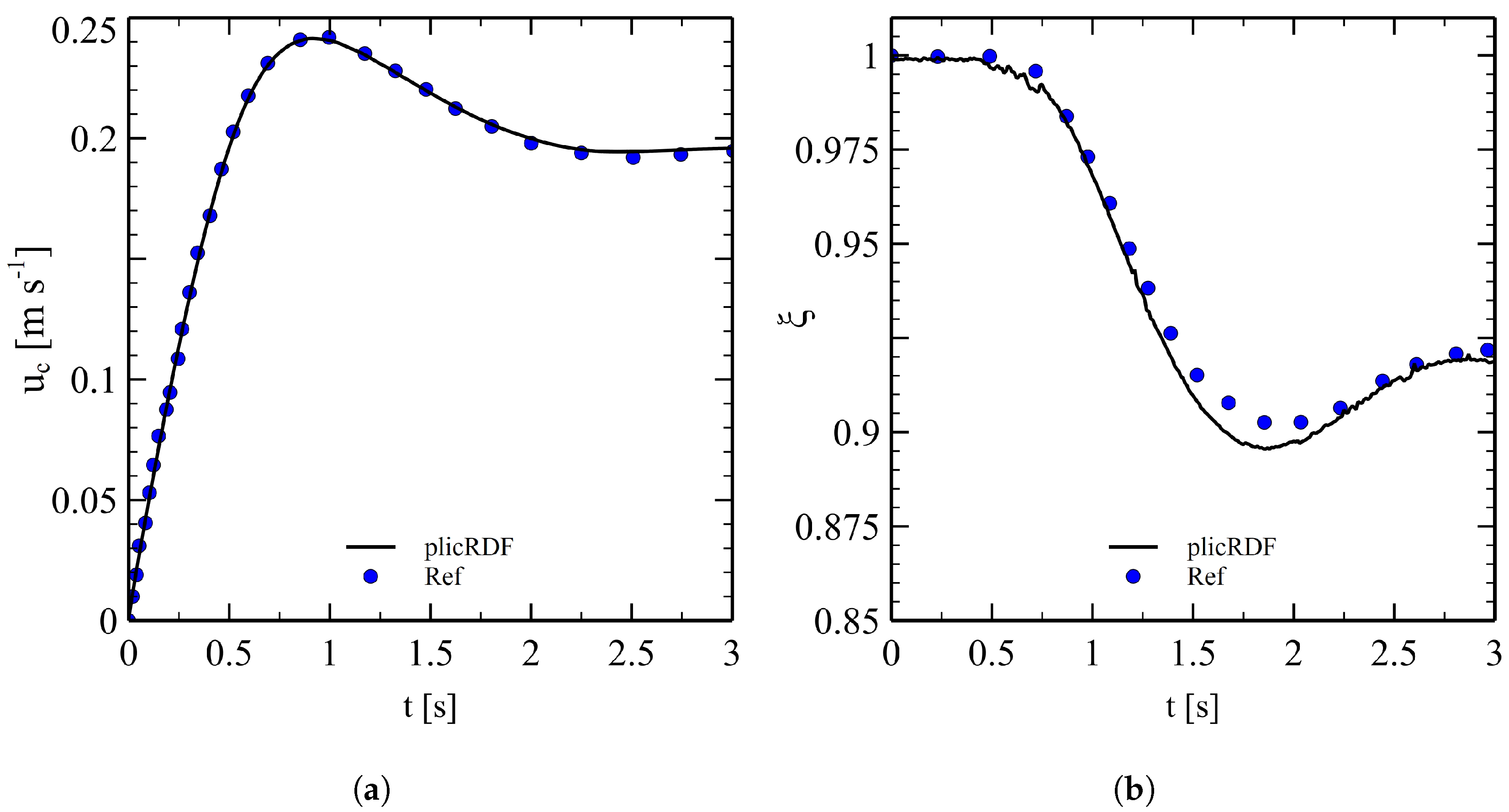
Figure 4 shows the evolution $u_c$ (Figure 4a) and $\xi$ (Figure 4b) provided by plicRDF on M4 mesh compared with Ref. [10], showing excellent agreement between the results of the two codes. As shown in Table 5, interIsoFoam provides results in close agreement for all the considered parameters and for both the code variants, which differ by a maximum of ≃$\pm 0.9\%$. The temporal evolution of $u_c$ provided by the code is practically coincident (Figure 4a) with respect to the reference one, while the circularity shows a slight discrepancy especially at ≃2 s and slight oscillations in some points (Figure 4b).

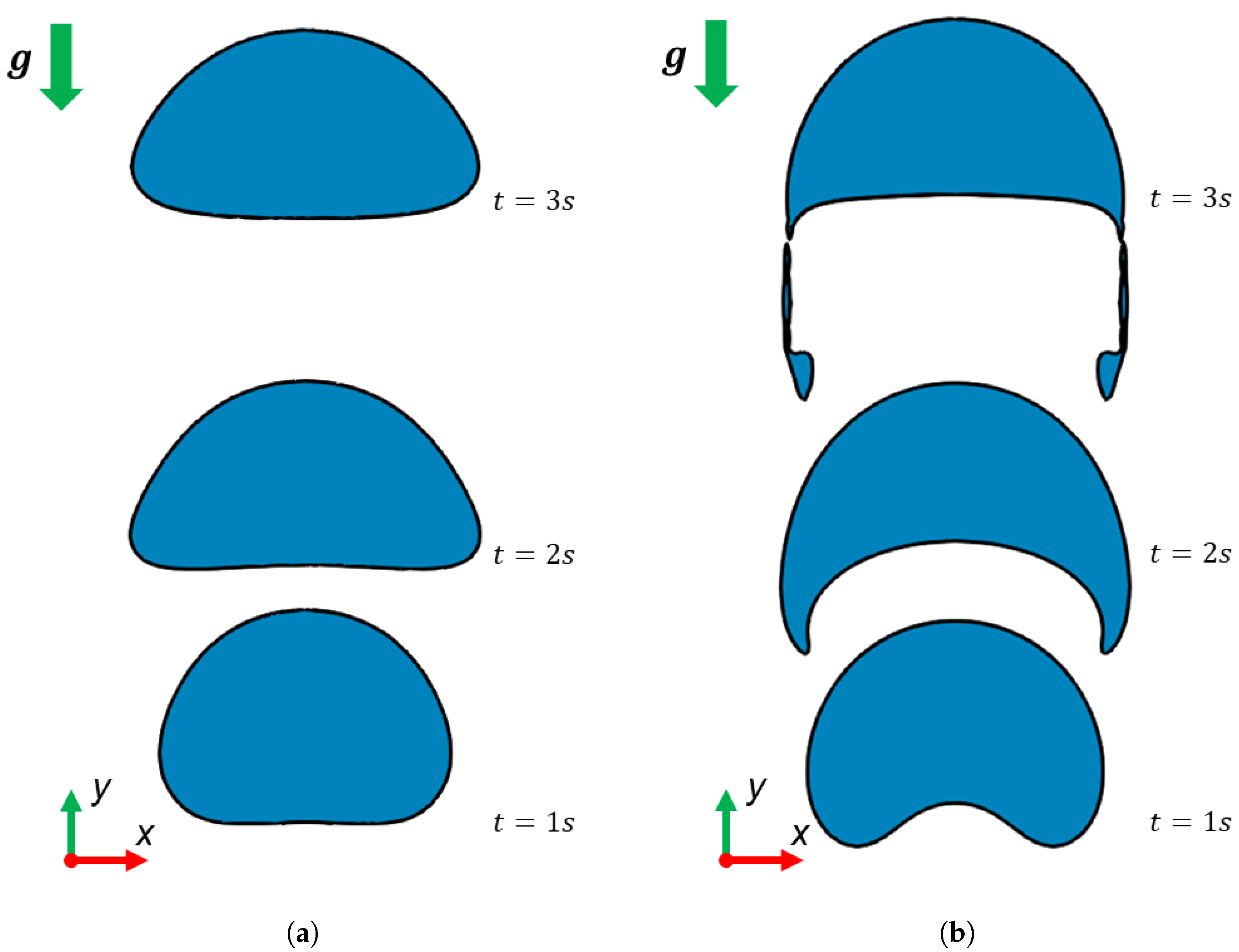
Figure 5a shows the bubble shapes at three different moments: the bubble, which is perfectly circular at $t=0$ s, is horizontally stretched during the rising while it is slightly compressed vertically, changing the curvature of the interface and assuming an ellipsoidal shape. Figure 5b shows the evolution of bubble shape for the C2 scenario, which is very different at this Eötvös number, with respect to the C1 case: the bubble immediately deforms in a more pronounced way ($t=1$ s) and progressively creates a skirt in its lower part ($t=2$ s). At the end of the rising ($t=3$ s), extremely thin filaments are generated, almost detached from the central body. As shown in Refs. [26,29], this is the most difficult region to simulate, where different codes provide different solutions: the filaments are more or less thin and may or may not detach. The mesh used, always triangular and unstructured, has 160 divisions along the x-axis and 320 along the y-axis.

Table 6. Benchmark results for the C2 case for both isoAlpha and pliRFD method compared with Ref. [29].

	${\mathit{\xi }}_{\mathit{min}}$	${\mathit{t}|}_{\mathit{\xi }={\mathit{\xi }}_{\mathit{min}}}$	${\mathit{u}}_{\mathit{c},\mathit{max}}$ (m s${}^{-1}$)	${\mathit{t}|}_{{\mathit{u}}_{\mathit{c}}={\mathit{u}}_{\mathit{c},\mathit{max}}}$	${\mathit{y}}_{\mathit{c}}$ (t = 3 s)
isoAlpha	0.4743	3.0000	0.2491	0.7170	1.1175
plicRDF	0.4725	3.0000	0.2491	0.7180	1.1175
TP2D	0.5869	2.4004	0.2524	0.7332	1.1380
FreeLIFE	0.4647	3.0000	0.2514	0.7281	1.1249
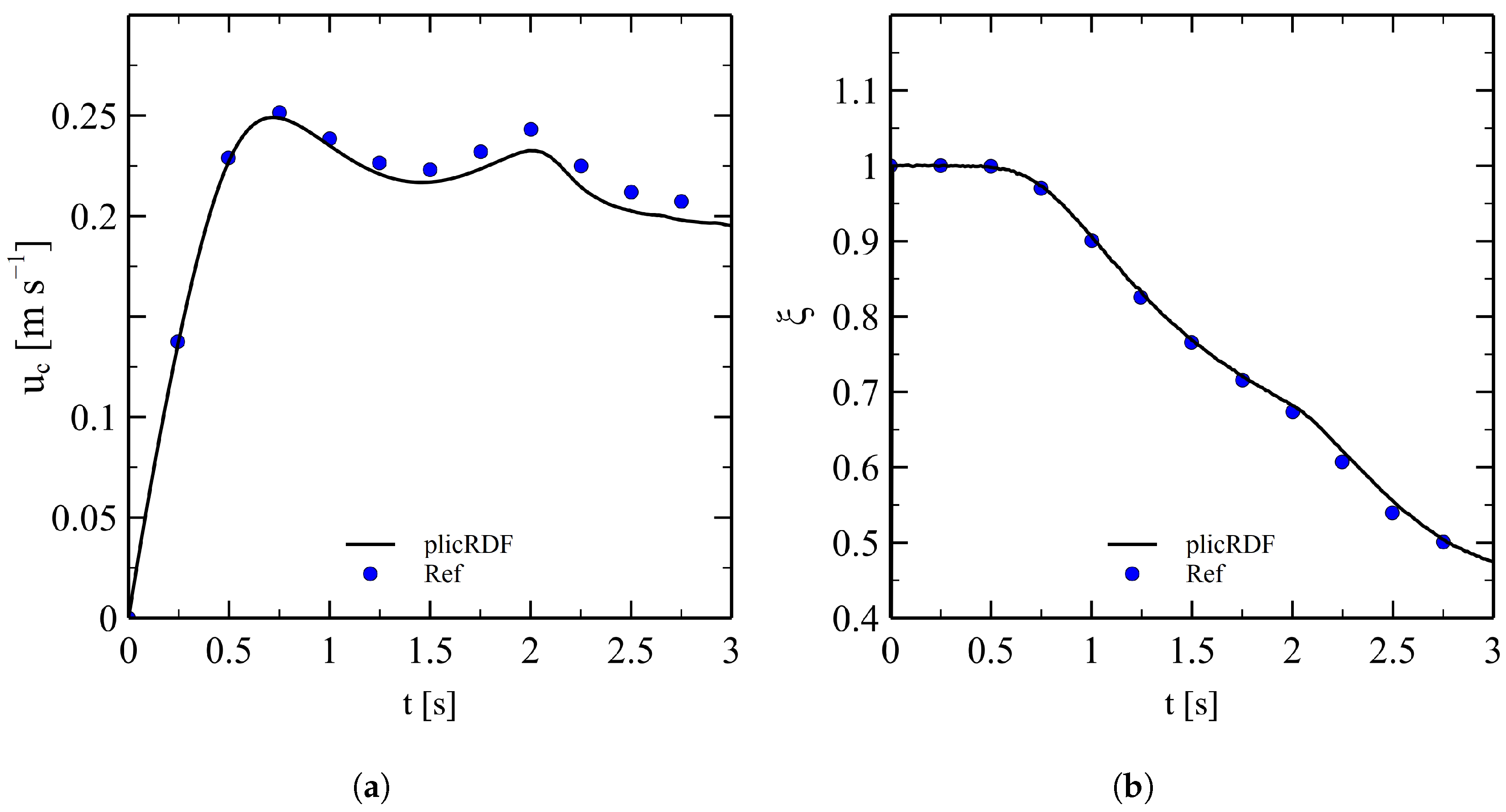
MooNMD	0.5144	3.0000	0.2502	0.7317	1.1376

shows the comparison between the results produced by the code, for both variants, and the three codes considered in Ref. [29]. The variants of the code provide almost identical results, while the comparison with the other codes confirms that the evaluation of the circularity, and therefore of the interface, is the most challenging parameter, where there is an absolute discrepancy of ≃24%, ≃9% and ≃2% respectively for the TP2D, MooNMD and FreeLIFE codes. For the other parameters the mean absolute error is about ≃1.4%. Figure 6a,b show, respectively, the evolution of $u_c$ and $\xi$ computed by the plicRDF solver and the FreeLIFE code [29], confirming the excellent agreement between the two codes for the entire transient.

3.1.3. 3D Rising Bubble

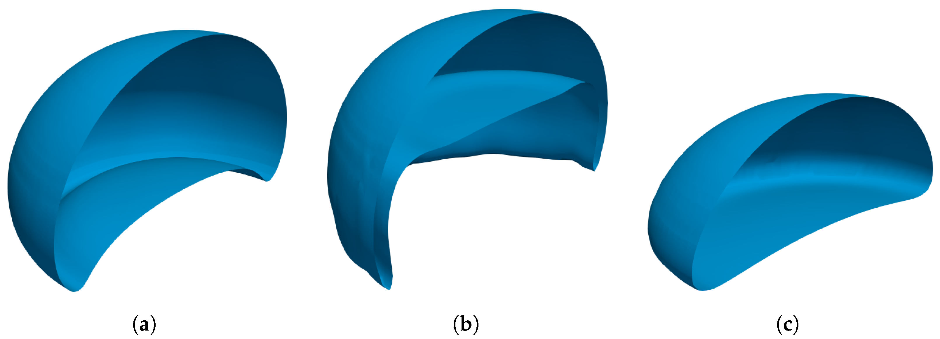
The third benchmark aims to prove the stability and accuracy of the code, in its plicRDF variant, by simulating the rise of a three-dimensional bubble for three different scenarios, for which characteristic parameters are collected in

Table 7. Parameters for the 3D rising bubble test.

	${\mathit{\eta }}_{\mathit{\rho }}$	${\mathit{\eta }}_{\mathit{\mu }}$	g (m s${}^{-2}$)	$\mathit{\gamma }$ (N m${}^{-1}$)	Eo	Mo
C1	100	100	9.81	8.37 × 10−3	116	41.1
C2	100	100	9.81	2.86 × 10−3	339	43.1
C3	714	6670	9.81	2.49 × 10−2	39.4	0.065

and whose shapes at the end of the transient are shown in Figure 7a–c for the scenarios C1, C2 and C3 respectively. As expected, as the Eötvös number increases, the deformation of the bubble increases, which assumes a “skirt” shape for the C3 case.

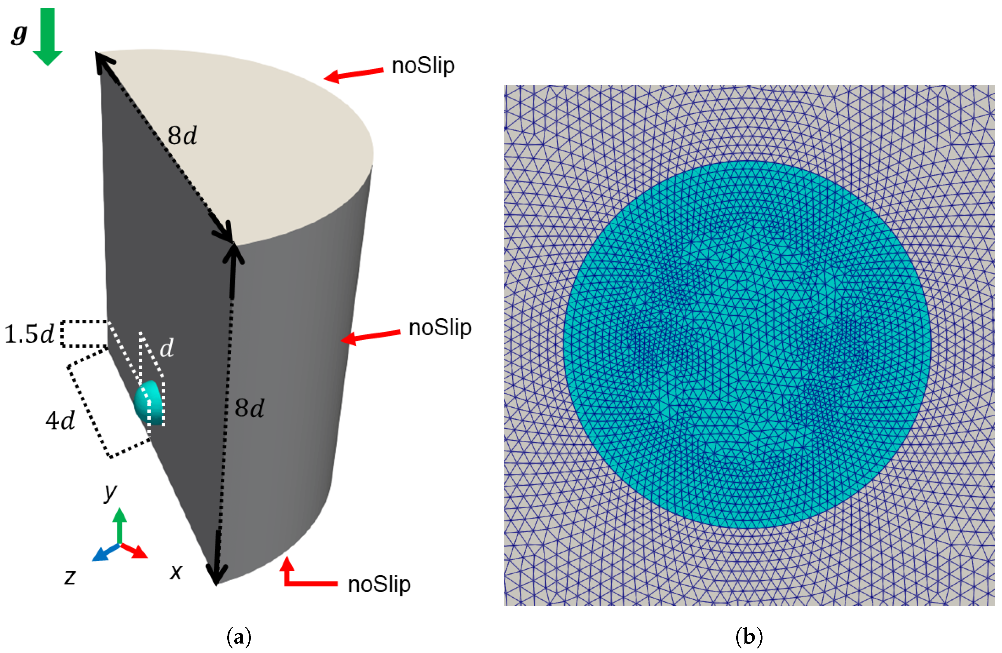
As shown in Figure 8a, the numerical domain is a cylinder of diameter and height $8d$, with d being the diameter of the bubble. The latter is centred in the lower part at a height equal to $1.5$d with respect to the lower face. The figure also shows the imposed BCs: noSlip condition for the velocity and zeroGradient for the pressure on all faces. The mesh used, shown in Figure 8b, is prismatic and unstructured. The mesh was generated from a 2D mesh extruded along the cylinder axis direction for a s number of steps. The resolution of the grid is greater around the axis of symmetry of the cylinder, where a uniform grid size h has been imposed, to maximize the resolution of the bubble. The mesh grows towards the edge of the cylinder, where the elements reach their maximum size. The same numerical setup described in Section 3.1.1 was used.

The control parameters used to evaluate the performance of the code are the velocity of the centroid, expressed through the Galilei number, and the sphericity $\mathsf{\Phi }$, which measures when the shape of the bubble deviates from the spherical one, to which it is associated $\mathsf{\Phi }=1$

$$\mathsf{\Phi }={\displaystyle \frac{{\left({\displaystyle \frac{3{\mathsf{\Omega }}_{{\alpha }_2}}{4\pi }}\right)}^{2/3}}{{\displaystyle \frac{A_{{\alpha }_2}}{4\pi }}}}$$

(20)

For case C1 (Table 7), a mesh sensitivity study was carried out considering four different meshes, with different resolution of the grid on the plane (h) and axial repartitions (s), as can be seen in

Table 8. Mesh data for 3D rising bubble C1 case mesh sensitivity study.

	Grid Size h (cm)	Axial Divisions s	Number of Elements
M1	0.067	120	222,720
M2	0.050	160	774,400
M3	0.033	240	2,881,200
M4	0.025	320	7,128,320

. The simulations were performed on the Sigmar server with between 18 and 24 processors and computational times were between about 1 h (mesh M1) and 54 hours (mesh M4). The parameters considered for the comparison are the Galilei number and the sphericity considering the scaled time $t^{*}=t/U_g$ [10]. As shown in

Table 9. Mesh sensitivity study results for 3D rising bubble C1 case. Absolute error E has as reference value that of the M4 mesh.

	$\mathbf{\Phi }$	${\mathit{E}}_{\mathbf{\Phi }}(\%)$	Ga	${\mathit{E}}_{Ga}(\%)$
M1	0.8341	2.807	7.0894	0.263
M2	0.8181	0.901	7.1176	0.134
M3	0.8126	0.234	7.1032	0.068
M4	0.8107	-	7.1080	-

, the average results in the final part of the transient ($7\le t^{*}\le 8$) produced for meshes M2, M3 and M4 differ by a maximum of $0.9\%$ and also in this case, similarly to what we discussed in Section 3.1.2 for the 2D bubble, the parameter that is most affected by the resolution of the mesh is the one directly linked to the resolution of the interface, that is the sphericity.

Table 10. Benchmark results for the 3D C1 case (M3 mesh) compared against numerical data from Refs. [10,30] and experimental data Ref. [31]. Absolute error E has as reference value the plicRDF values.

	Ga	${\mathit{E}}_{Ga}(\%)$	$\mathbf{\Phi }$	${\mathit{E}}_{\mathbf{\Phi }}(\%)$
pliRDF	7.09	-	0.82	-
Ref. [10]	7.02	0.98	0.81	0.71
Ref. [31]	7.16	1.00	-	-
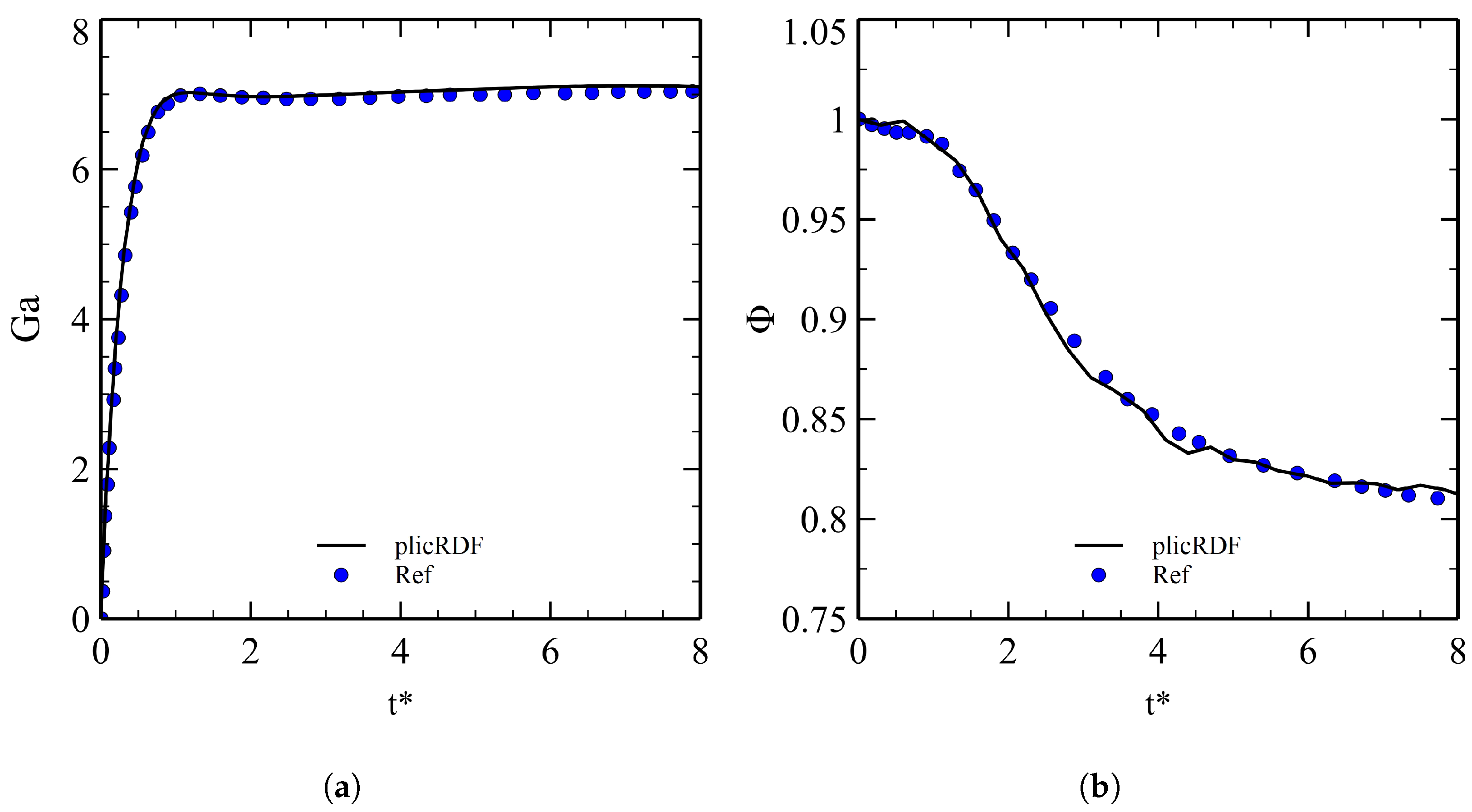
Ref. [30]	7.0	1.27	-	-

compares the results for C1 case with the numerical results presented in Refs. [10,30] and with the experimental data reported in Ref. [31]. Since the exact time of the evaluation of the parameters is not reported in the references considered, the algebraic average of the values $7\le t^{*}\le 8$ was considered. The code provides results in great agreement with both numerical and experimental results. Figure 9a,b show, respectively, the time evolution of Ga and $\mathsf{\Phi }$ and comparing it with the data presented in Ref. [10], showing great agreement between the results throughout the transient.

Table 11. Benchmark results for the 3D C2 case (M4 mesh) compared against numerical data from Refs. [10,30] and experimental data Ref. [31]. Absolute error E has as reference value the plicRDF values.

	Ga	${\mathit{E}}_{Ga}(\%)$
pliRDF	17.88	-
Ref. [10]	17.64	1.36
Ref. [30]	17.91	0.17
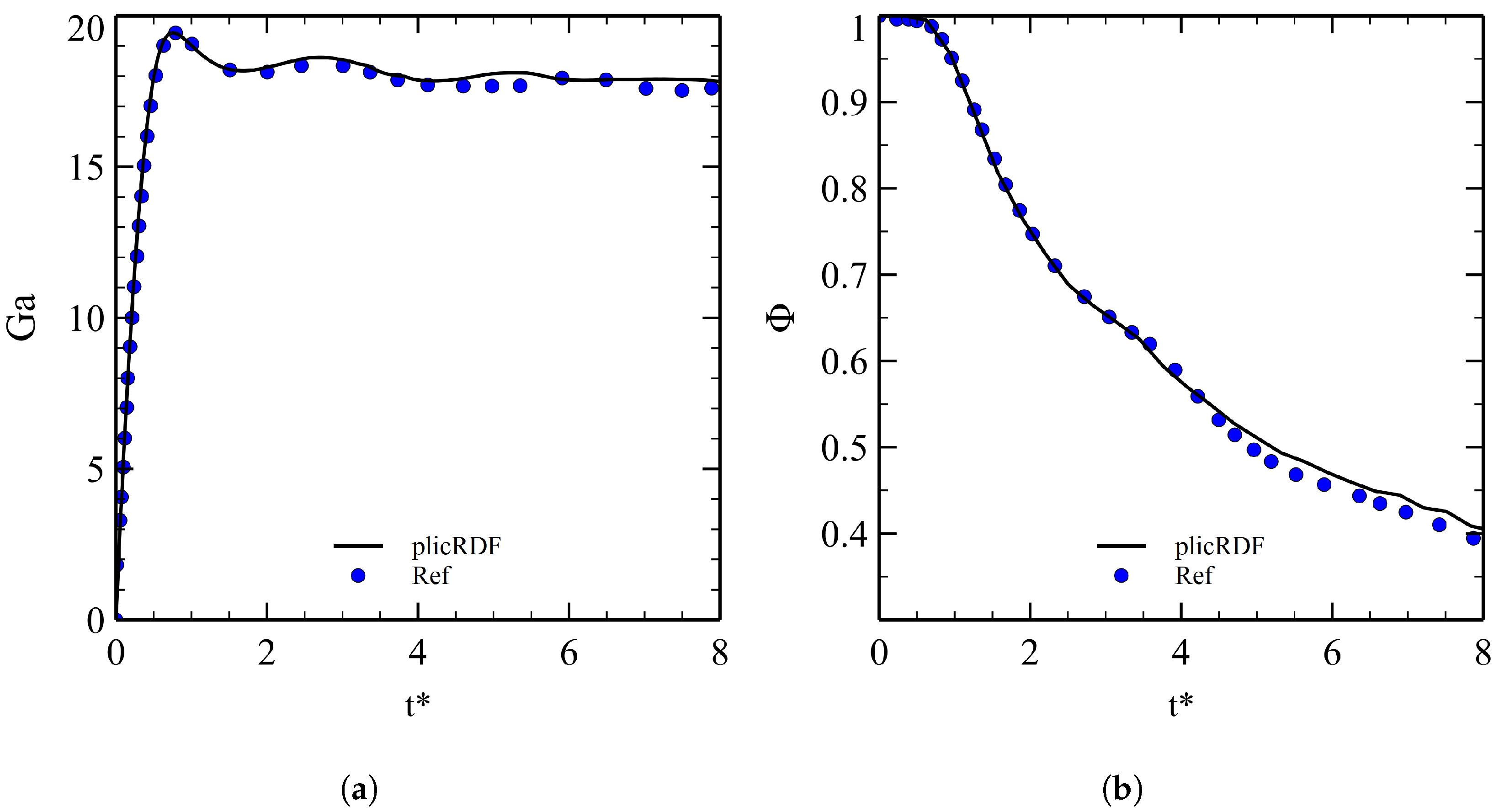
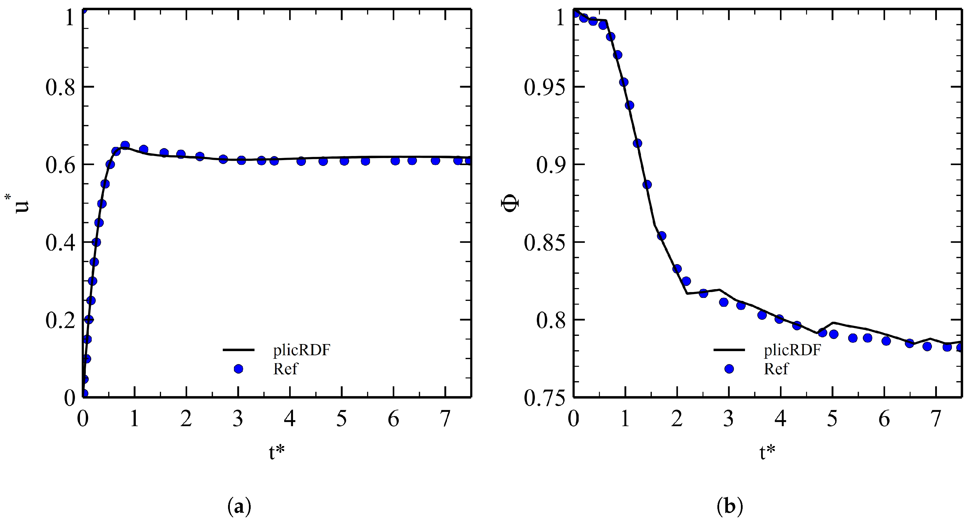
Ref. [31]	18.3	2.30

compares the results for C2 case with the numerical results presented in Refs. [10,30] and with the experimental data reported in Ref. [31] considering the average values in the time window $7\le t^{*}\le 8$, whereas Figure 10a,b show, respectively, the time evolution of Ga and $\mathsf{\Phi }$ and comparing it with the data presented in Ref. [10]. Even in this regime, the code provides excellent results. Finally,

Table 12. Benchmark results for the 3D C3 case (M3 mesh) compared against numerical data from Ref. [10] and experimental data Ref. [32]. Absolute error E has as reference value the plicRDF values. $u^{*}=u_y/U_g$.

	${\mathit{u}}^{*}$	${\mathit{E}}_{{\mathit{u}}^{*}}(\%)$
pliRDF	0.6195	-
Ref. [10]	0.6110	1.40
Ref. [32]	0.6226	0.49

compares the results for C3 case, that presents the highest density ratio (${\eta }_{\rho }=714$) with the numerical results presented in Ref. [10] and with the experimental data reported in Ref. [32] considering the average values in the time window $7\le t^{*}\le 8$, this time, the scaled velocity $u^{*}=u/U_g$ is considered instead of Galilei number. The code shows great agreement with respect to the experimental data, with an error of less than $0.5\%$. Figure 11a,b show, respectively, the time evolution of $u^{*}$ and $\mathsf{\Phi }$ and the same reported in Ref. [10].

3.1.4. Co-Axial Coalescence of Two Bubbles

The last benchmark is the co-axial coalescence of two bubbles. The computational domain and the mesh used are the same represented, respectively, in Figure 8a,b, where M3 mesh was used (Table 8). The BCs and the numerical set up are also the same presented in Section 3.1.3. The second bubble, initialized using the setAlphaField utility, has the same diameter d as the first bubble shown Figure 8a and is positioned aligned with it with respect to the y-direction at a distance from its centroid equal to $1.5d$. The characteristic parameters for this case are: $Eo=16,Mo=2 \times {10}^{-4},{\eta }_{\rho }=100$ and ${\eta }_{\mu }=100$.

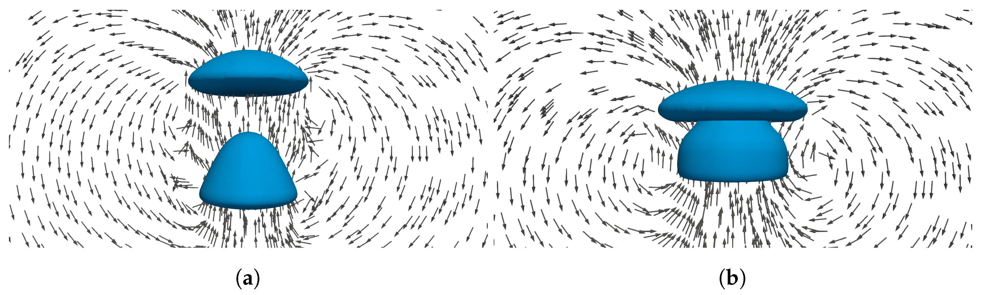
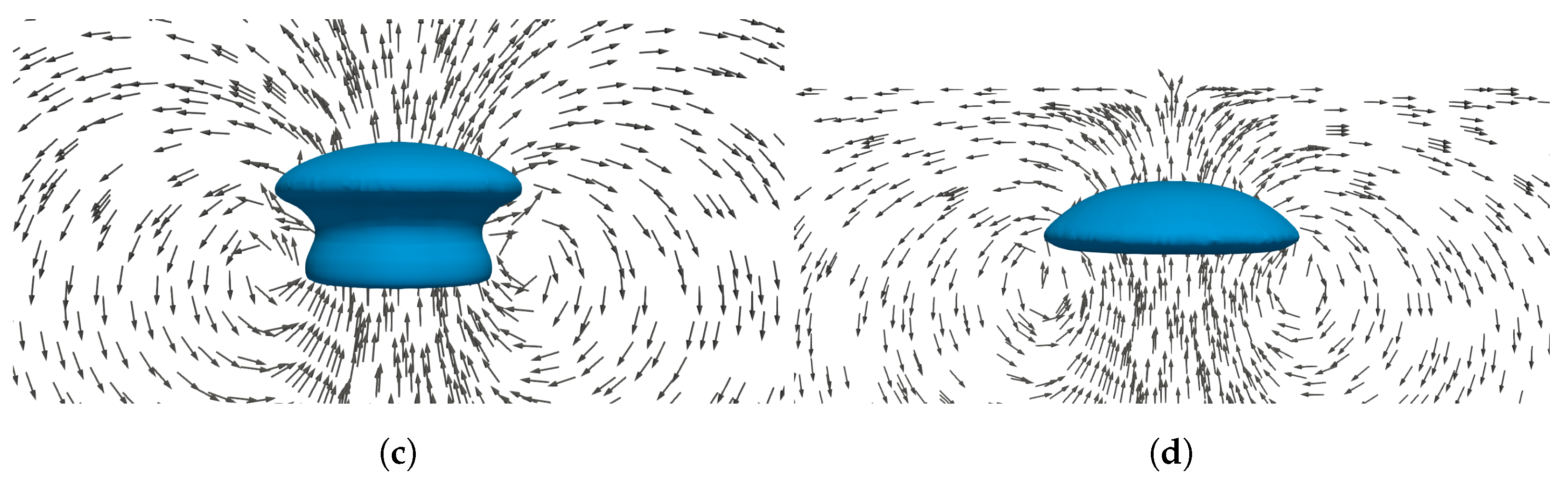
Figure 12 shows four snapshots of the topological change of the interface during the coalescence process. The leading bubble creates a depression in the area below, generating the suction on the following bubble which deforms along the vertical direction and accelerates (Figure 12a). As the motion progresses, the bubbles touch and begin to coalesce starting from a small portion of the interface centred on the axis passing through the bubble centroids (Figure 12b) which expands rapidly generating a mushroom-like structure (Figure 12c). Finally, the bubbles fully coalesce (Figure 12d).

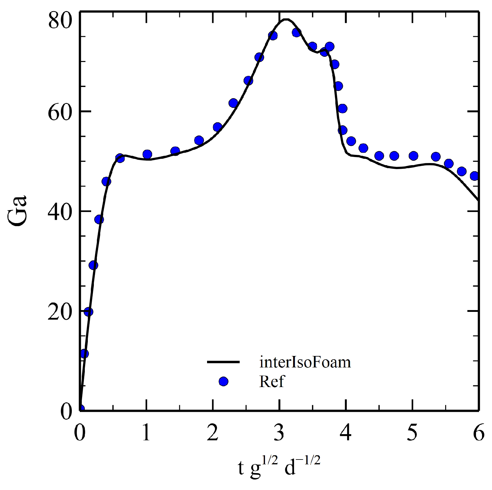
As shown in Figure 13, the numerical prediction of the evolution of the rising velocity (Galilei number) is in great agreement with that provided by the VFO/level-set code used in Ref. [10]. Indeed, the value of the absolute error relative to the maximum Galilei number (at ≃ 3 s) and the absolute integral error between the two curves are equal, respectively, to ≃2.77% and to ≃2.64%. Moreover, the bubble shapes showed in Figure 12 is consistent with the experimental results reported in Ref. [33] and with the VOF simulation from Ref. [34] and level-set simulation from Ref. [35].

3.2. Rising He Bubble in PbLi

In the second phase of the research activity, the code was tested with the real properties of the He-PbLi mixture at representative conditions as those likely encountered during the blanket normal operation (327 °C and 1 bar) since, considering a higher pressure due to the hydraulic head, the density ratio decreases as the density of the helium increases but that of the PbLi remains practically unchanged. This mixture has an extremely high density ratio (${\eta }_{\rho }=1.24 \times {10}^5$) and, to the best of our knowledge, this is the first attempt at simulating a two-phase flow with such high ${\eta }_{\rho }$. As no experimental or numerical data are available, a qualitative benchmark was carried out, simulating 2D bubbles of different diameters which fall within different regimes. The first experimental studies that investigated the regimes of a rising bubble in viscous liquids date back to the early 80s from the seminal works by Clift et al. [36] and Bhaga and Weber [31]. Recently, Tripathi et al. [37] and Sharaf et al. [38] have conducted, respectively, a numerical and experimental campaign considering the rising of an air bubble in a solution of water and glycerol for a wide range of Ga and Eo numbers, essentially identifying five fundamental regimes: axisymmetric, skirted, oscillatory, peripheral breakup and central breakup.

Table 13. Parameters for the H rising bubble in PbLi analyses.

	$\mathit{d}/2$ (mm)	${\mathit{\eta }}_{\mathit{\rho }}$	${\mathit{\eta }}_{\mathit{\mu }}$	Ga	Eo
B1	0.2	1.24 × 105	61	44	8.44 × 10−3
B2	116	5.00 × 104	100	12	4.86 × 103
B3	1	1.24 × 105	61	497	0.21
B4	10	1.24 × 105	61	1.57 × 104	21.1
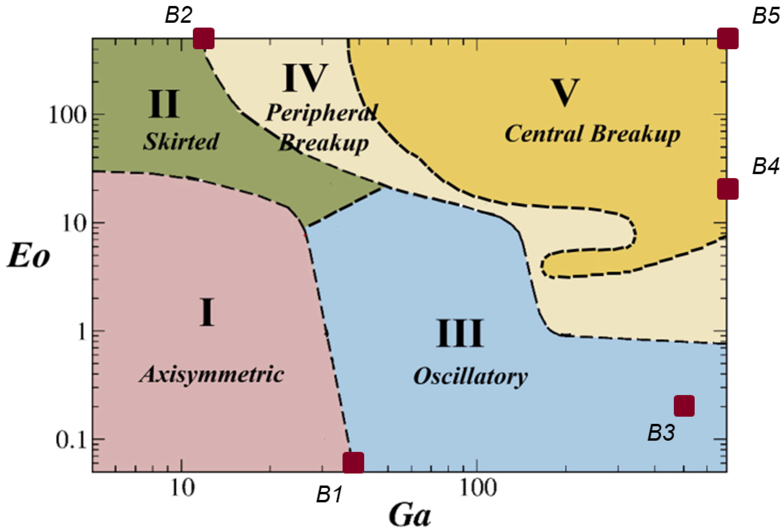
B5	100	1.24 × 105	61	4.97 × 105	2.11 × 103

shows the parameters of the five bubbles tested, while Figure 14 qualitatively shows their positioning in the phase plot diagram presented in Ref. [38]. The density and the dynamic viscosity at 327 °C and 1 bar for the helium and the PbLi are, respectively, ${\rho }_{He}=0.0791\mathrm{kg}{\mathrm{m}}^3$ [39], ${\mu }_{He}=3.20\times {10}^{-5}\mathrm{Pa}\mathrm{s}$ [40] and ${\rho }_{PbLi}=9806\mathrm{kg}{\mathrm{m}}^3$, ${\mu }_{PbLi}=1.96\times {10}^{-3}\mathrm{Pa}\mathrm{s}$. It must be emphasized that the B2 bubble was not simulated with the real properties of the He-PbLi mixture, but with a fictitious mixture (${\rho }_{{\alpha }_1}=1000\mathrm{kg}{\mathrm{m}}^3,{\nu }_{{\alpha }_1}=0.01{\mathrm{m}}^2\mathrm{s},\gamma =0.271\mathrm{N}{\mathrm{m}}^{-1}$) which, in any case, has a density ratio relevant to the study (Table 13). The computational domain, the mesh used (M3, Table 3), the BCs, the ICs and the numerical setup are the same used for the study in Section 3.1.2 with the only difference that the gravity acceleration is equal to 9.81 m s${}^2$.

The computational times, considering 4 processors in parallel, vary between about 7 and 85 h depending on the complexity of the bubble shape, where the cases in which the filaments are created and where the breakup is present require much smaller time-steps to guarantee the simulation stability, of the order of $1\times {10}^{-7}$ s, and therefore greater computational times. Regarding the computational efforts to simulate a high-density ratio case, it was found that, for ${\eta }_{\rho }>1000$, this parameter no longer influences the dynamics of the bubble. It is therefore possible to simulate a scenario with ${\eta }_{\rho }\gg 1000$, such as the He-PbLi one, by imposing an ${\eta }_{\rho }=1000$ (all other parameters being equal) which requires a much smaller number of iterations of the pressure solver, saving computational resources. A test was carried out by simulating two bubbles with $Eo=21,Ga=1.6 \times {10}^4,{\eta }_{\mu }=61$ and one bubble with ${\eta }_{\rho }=1.2 \times {10}^5$ and the other with ${\eta }_{\rho }=1000$ for the same computational time (3 s) and with the same mesh. The bubble dynamics are extremely similar, with a maximum discrepancy of 10% considering the rising velocity and the circularity, but the computational time passes from $1.3\times {10}^5$ s to $6.6\times {10}^3$ s (≃$-95\%$) decreasing ${\eta }_{\rho }$.

3.2.1. Axisymmetric and Skirted Regimes

For low Ga and Eo the regime is axisymmetric (Figure 14), in which the bubble rises regularly while maintaining azimuthal symmetry and shape that, for increasing Eo, passes from spherical, to oblate and to dimple [38]. As shown in Figure 15a, for the B1 bubble the code provides a non-optimal result as there are some oscillations of the interface, which should be perfectly spherical given the very low Eo, and thus can be considered non-physical. This is essentially due to the generation of spurious velocities which, for low Eo numbers, have a great impact on the interface shape.

For low Ga and high Eo we have the skirted regime (Figure 14). The bubble deforms a lot during the rising, forming a cavities in the lower part and generating a thin peripheral edge that resembles a skirt [38]. As shown in Figure 15b, for the B2 bubble the code provides a consistent result, with the skirt starting to form at $t^{*}=3.96$ and, at the final time, it is almost separated from the central body, reflecting the fact that we are on the border between the skirted regime and the peripheral breakup (Figure 14). The interface has no spurious deformations.

3.2.2. Oscillatory Regime

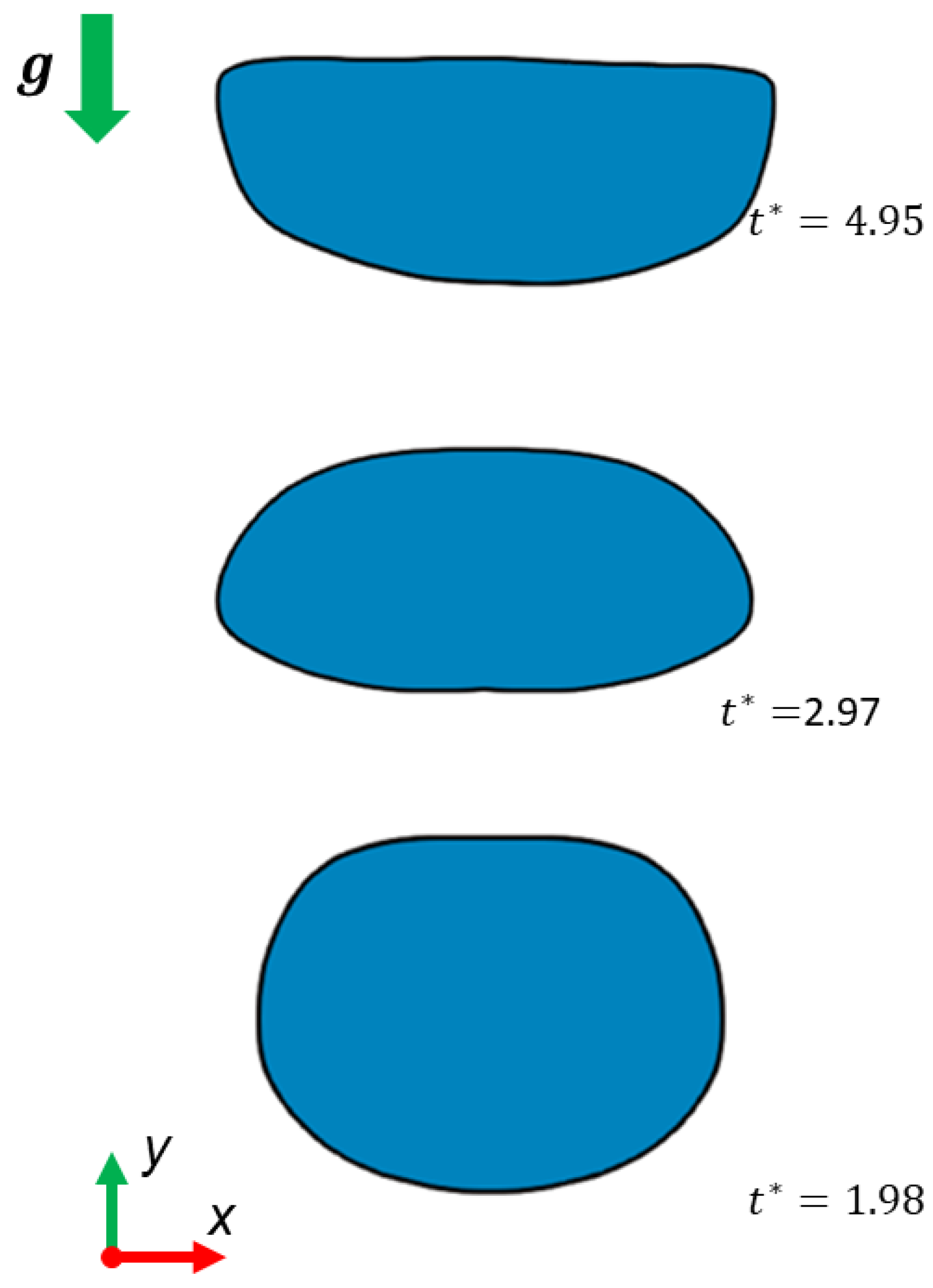
For high Ga and low Eo the rise of the bubble becomes irregular, generating a spiral or zigzag motion and the regime becomes oscillatory [38]. As shown in Figure 16, also in this case, being $Eo<1$ for the B3 bubble, the code provides an irregular interface, deformed by the spurious velocities, but reproduces the expected irregular trend, reversing the direction of the concavity passing from $t^{*}=2.97$ to $t^{*}=4.95$.

3.2.3. Peripheral and Central Breakup Regimes

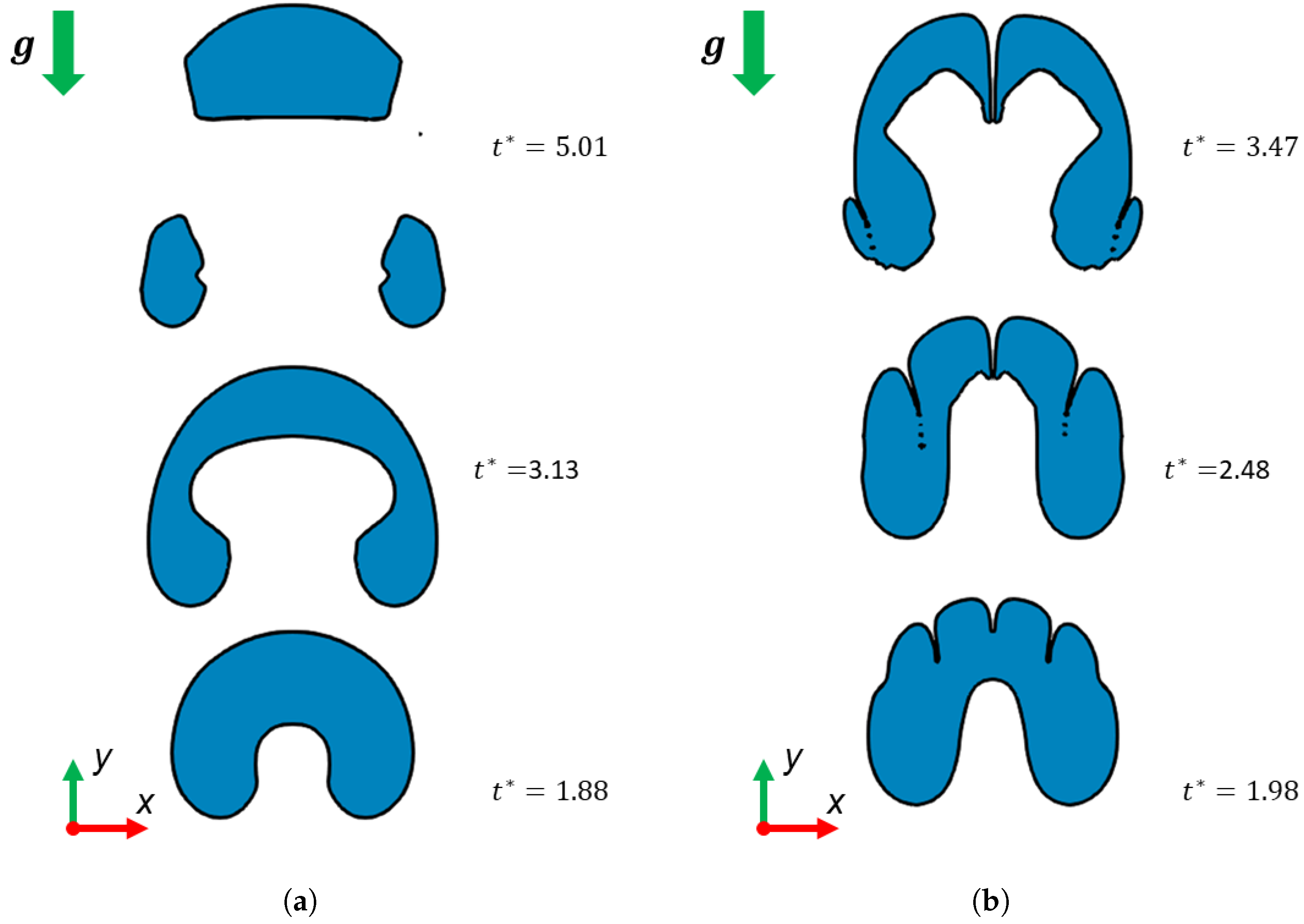
For high Ga and Eo the surface tension is unable to oppose the gravitational force and the bubble tends to split into satellite bubbles which, having a smaller diameter, have smaller Ga and Eo and thus do not break further. Peripheral breakup occurs when the split occurs at the periphery of the bubble. As shown in Figure 17a, the code gives a consistent result with this regime for bubble B4, whose position is outside the phase plot showed in Figure 14 but, considering the shape of zone IV for high Ga, it seems reasonable to think that it is the effective regime.

Central breakup occurs when the bubble first assumes a toroidal shape and then split from the centre, with no other significant gaseous regions forming soon after rupture [38]. This regime has been identified only in numerical simulations [37], probably because it occurs only if the initial shape is perfectly spherical, a situation of difficult experimental reproduction [38]. As shown Figure 17b, the code provides a consistent solution with this regime.

4. Conclusions

The interIsoFoam solver was validated for a 2D stationary drop, 2D rising bubble, 3D rising bubble and for the co-axial coalescence of two bubbles, comparing the results obtained with both numerical and experimental results. The code returned excellent results in almost all the cases tested, but has not been particularly accurate for the stationary case, where an error of about 10% was observed in the evaluation of the pressure jump. This discrepancy is due to an inaccurate resolution of the interface, which generates spurious velocities that impact the force balance between the pressure and the surface tension on the interface. This situation can be mitigated by increasing the number of iterations in the reconstructor-step of the plicRFD method, it is therefore interesting to carry out further simulations considering the improvement of the error with respect to computational time, which increases with the number of iterations.

Subsequently, the solver was tested for a high density ratio mixture, simulating the rising of a helium bubble in the PbLi at different rates of motion [37,38]. The solver was able to provide consistent results with the expected regimes in all the five cases tested. Also in this situation, for Eötvös numbers lower than unity, which correspond to low velocities of the surrounding fluid, we can see the impact of the spurious velocities on the interface, which however do not seem to influence the dynamics of the bubble.

Overall, interIsoFoam has proven to be able to correctly simulate the basic characteristics of a flow with a high density ratio, therefore it is an excellent candidate for the future implementation of the MHD equations, following the methodology presented by Zhang et al. [41], for the study of the migration of helium bubbles in the blanket [2,3], but also in the framework of the advanced PFCs [17,18,19].

References

- Kikuchi, M.; Lackner, K.; Quang, M. Fusion Physics; International Atomic Energy Agency (IAEA): Vienna, Austria, 2012. [Google Scholar]
- Batet, L.; Fradera, J.; Valls, E.M.D.L.; Sedano, L.A. Numeric implementation of a nucleation, growth and transport model for helium bubbles in lead-lithium HCLL breeding blanket channels: Theory and code development. Fusion Eng. Des. 2011, 86, 421–428. [Google Scholar] [CrossRef]
- Kordač, M.; Košek, L. Helium bubble formation in Pb-16Li within the breeding blanket. Fusion Eng. Des. 2017, 124, 700–704. [Google Scholar] [CrossRef]
- Prosperetti, A.; Tryggvason, G. Computational Methods for Multiphase Flow; Cambridge University Press: Cambridge, UK, 2007. [Google Scholar] [CrossRef] [Green Version]
- Hirt, C.W.; Nichols, B.D. Volume of fluid (VOF) method for the dynamics of free boundaries. J. Comput. Phys. 1981, 39, 201–225. [Google Scholar] [CrossRef]
- Osher, S.; Sethian, J.A. Fronts propagating with curvature-dependent speed: Algorithms based on Hamilton-Jacobi formulations. J. Comput. Phys. 1988, 79, 12–49. [Google Scholar] [CrossRef] [Green Version]
- Deshpande, S.S.; Anumolu, L.; Trujillo, M.F. Evaluating the performance of the two-phase flow solver interFoam. Comput. Sci. Discov. 2012, 5, 014016. [Google Scholar] [CrossRef]
- Cummins, S.J.; Francois, M.M.; Kothe, D.B. Estimating curvature from volume fractions. Comput. Struct. 2005, 83, 425–434. [Google Scholar] [CrossRef]
- Wang, Z.; Yang, J.; Stern, F. An improved particle correction procedure for the particle level set method. J. Comput. Phys. 2009, 228, 5819–5837. [Google Scholar] [CrossRef]
- Balcázar, N.; Lehmkuhl, O.; Jofre, L.; Rigola, J.; Oliva, A. A coupled volume-of-fluid/level-set method for simulation of two-phase flows on unstructured meshes. Comput. Fluids 2016, 124, 12–29. [Google Scholar] [CrossRef] [Green Version]
- Nave, J.C.; Rosales, R.R.; Seibold, B. A gradient-augmented level set method with an optimally local, coherent advection scheme. J. Comput. Phys. 2010, 229, 3802–3827. [Google Scholar] [CrossRef] [Green Version]
- Francois, M.M.; Cummins, S.J.; Dendy, E.D.; Kothe, D.B.; Sicilian, J.M.; Williams, M.W. A balanced-force algorithm for continuous and sharp interfacial surface tension models within a volume tracking framework. J. Comput. Phys. 2006, 213, 141–173. [Google Scholar] [CrossRef]
- Tryggvason, G.; Scardovelli, R.; Zaleski, S. Direct Numerical Simulations of Gas–Liquid Multiphase Flows; Cambridge University Press: Cambridge, UK, 2011. [Google Scholar]
- Zhang, C.; Eckert, S.; Gerbeth, G. Experimental study of single bubble motion in a liquid metal column exposed to a DC magnetic field. Int. J. Multiph. Flow 2005, 31, 824–842. [Google Scholar] [CrossRef]
- Schwarz, S.; Fröhlich, J. Numerical study of single bubble motion in liquid metal exposed to a longitudinal magnetic field. Int. J. Multiph. Flow 2014, 62, 134–151. [Google Scholar] [CrossRef]
- Zhang, J.; Ni, M.J. A numerical study of a bubble pair rising side by side in external magnetic fields. J. Fluid Mech. 2021, 926. [Google Scholar] [CrossRef]
- Kessel, C.E.; Andruczyk, D.; Blanchard, J.P.; Bohm, T.; Davis, A.; Hollis, K.; Humrickhouse, P.W.; Hvasta, M.; Jaworski, M.; Jun, J.; et al. Critical Exploration of Liquid Metal Plasma-Facing Components in a Fusion Nuclear Science Facility. Fusion Sci. Technol. 2019, 75, 886–917. [Google Scholar] [CrossRef]
- Smolentsev, S.; Rognlien, T.; Tillack, M.; Waganer, L.; Kessel, C. Integrated Liquid Metal Flowing First Wall and Open-Surface Divertor for Fusion Nuclear Science Facility: Concept, Design, and Analysis. Fusion Sci. Technol. 2019, 75, 939–958. [Google Scholar] [CrossRef]
- Siriano, S.; Tassone, A.; Caruso, G. Numerical Simulation of Thin-Film MHD Flow for Nonuniform Conductivity Walls. Fusion Sci. Technol. 2021, 77, 144–158. [Google Scholar] [CrossRef]
- OpenFOAM: User Guide. Available online: https://www.openfoam.com/documentation/user-guide (accessed on 27 March 2022).
- Weller, H.G. A New Approach to VOF-Based Interface Capturing Methods for Incompressible and Compressible Flow; Report TR/HGW; OpenCFD Ltd.: Bracknell, UK, 2008; Volume 4. [Google Scholar]
- Roenby, J.; Bredmose, H.; Jasak, H. A computational method for sharp interface advection. R. Soc. Open Sci. 2016, 3, 160405. [Google Scholar] [CrossRef] [PubMed] [Green Version]
- Roenby, J.; Bredmose, H.; Jasak, H. Isoadvector: Geometric vof on general meshes. In OpenFOAM—Selected Papers of the 11th Workshop; Springer: Cham, Switzerland, 2019; pp. 281–296. [Google Scholar] [CrossRef]
- Scheufler, H.; Roenby, J. Accurate and efficient surface reconstruction from volume fraction data on general meshes. J. Comput. Phys. 2019, 383, 1–23. [Google Scholar] [CrossRef] [Green Version]
- Brackbill, J.U.; Kothe, D.B.; Zemach, C. A continuum method for modeling surface tension. J. Comput. Phys. 1992, 100, 335–354. [Google Scholar] [CrossRef]
- Gamet, L.; Scala, M.; Roenby, J.; Scheufler, H.; Pierson, J.L. Validation of volume-of-fluid OpenFOAM® isoAdvector solvers using single bubble benchmarks. Comput. Fluids 2020, 213, 104722. [Google Scholar] [CrossRef]
- Hysing, S. Mixed element FEM level set method for numerical simulation of immiscible fluids. J. Comput. Phys. 2012, 231, 2449–2465. [Google Scholar] [CrossRef]
- Popinet, S. Numerical Models of Surface Tension. Annu. Rev. Fluid Mech. 2018, 50, 49–75. [Google Scholar] [CrossRef] [Green Version]
- Hysing, S.; Turek, S.; Kuzmin, D.; Parolini, N.; Burman, E.; Ganesan, S.; Tobiska, L. Quantitative benchmark computations of two-dimensional bubble dynamics. Int. J. Numer. Methods Fluids 2009, 60, 1259–1288. [Google Scholar] [CrossRef]
- Hua, J.; Stene, J.F.; Lin, P. Numerical simulation of 3D bubbles rising in viscous liquids using a front tracking method. J. Comput. Phys. 2008, 227, 3358–3382. [Google Scholar] [CrossRef] [Green Version]
- Bhaga, D.; Weber, M.E. Bubbles in viscous liquids: Shapes, wakes and velocities. J. Fluid Mech. 1981, 105, 61–85. [Google Scholar] [CrossRef] [Green Version]
- Hnat, J.G.; Buckmaster, J.D. Spherical cap bubbles and skirt formation. Phys. Fluids 1976, 19, 182–194. [Google Scholar] [CrossRef]
- Brereton, G.; Korotney, D. Coaxial and oblique coalescence of two rising bubbles. Dyn. Bubbles Vortices Near Free. Surf. 1991, 119, 50–73. [Google Scholar]
- Numerical simulation of gas bubbles behaviour using a three-dimensional volume of fluid method. Chem. Eng. Sci. 2005, 60, 2999–3011. [CrossRef]
- Balcázar, N.; Jofre, L.; Lehmkuhl, O.; Castro, J.; Rigola, J. A finite-volume/level-set method for simulating two-phase flows on unstructured grids. Int. J. Multiph. Flow 2014, 64, 55–72. [Google Scholar] [CrossRef]
- Clift, R.; Grace, J.; Weber, M. Bubbles, Drops and Particles; Dover Publications, Inc.: New York, NY, USA, 1978. [Google Scholar]
- Tripathi, M.K.; Sahu, K.C.; Govindarajan, R. Dynamics of an initially spherical bubble rising in quiescent liquid. Nat. Commun. 2015, 6, 6268. [Google Scholar] [CrossRef] [Green Version]
- Sharaf, D.M.; Premlata, A.R.; Tripathi, M.K.; Karri, B.; Sahu, K.C. Shapes and paths of an air bubble rising in quiescent liquids. Phys. Fluids 2017, 29, 122104. [Google Scholar] [CrossRef] [Green Version]
- The Engineering ToolBox. Helium—Density and Specific Weight. Available online: https://www.engineeringtoolbox.com/helium-density-specific-weight-temperature-pressure-d_2090.html (accessed on 27 March 2022).
- The Engineering ToolBox. Gases—Dynamic Viscosity. Available online: https://www.engineeringtoolbox.com/gases-absolute-dynamic-viscosity-d_1888.html (accessed on 27 March 2022).
- Zhang, J.; Ni, M.J. Direct simulation of multi-phase MHD flows on an unstructured Cartesian adaptive system. J. Comput. Phys. 2014, 270, 345–365. [Google Scholar] [CrossRef]
Figure 1.
Computational domain, BCs, ICs (a) and the detail of the mesh at the interface for the 2D static drop (b). Red colour corresponds to whereas the blue one to .
Figure 2.
Pressure profile on the horizontal axis passing through the centre of the model (a) and velocity vectors on the upper-right quarter, representing the spurious velocities, for the M3 mesh () (b).
Figure 3.
Computational domain, BCs, ICs (a) and mesh detail on the bubble at (b) for the 2D rising bubble test. The black line in (b) is the contour.
Figure 4.
Evolution of (a) and (b) for the C1 case provided by plicRDF on M4 mesh compared with Ref. [10].
Figure 5.
2D bubble shape evolution for the C1 (a) and C2 (b) scenario represented through contour .
Figure 6.
Evolution of (a) and (b) for the 2D C2 case provided by plicRDF compared with FreeLIFE code in Ref. [29].
Figure 7.
Bubble shape at the end of the transient for cases C1 (a), C2 (b) and C3 (c) represented through the half contour .
Figure 8.
Half computational domain, BCs, ICs (a) and mesh detail on the xz plane that cuts the bubble in half at (b) for the 3D rising bubble test. The bubble, coloured in cyan, is represented through the isovolume .
Figure 9.
Evolution of Ga (a) and (b) for the 3D C1 case provided by plicRDF (M4 mesh) compared with Ref. [10].
Figure 10.
Evolution of Ga (a) and (b) for the 3D C2 case provided by plicRDF compared with Ref. [10].
Figure 11.
Evolution of (a) and (b) for the 3D C3 case provided by plicRDF compared with Ref. [10].
Figure 12.
Bubble shapes for the coalescence test represented through the half contour , with velocity vectors, at four different times: (a), (b), (c) and (d).
Figure 13.
Evolution of Ga for the coalescence case provided by plicRDF compared with Ref. [10].
Figure 14.
Water-air phase plot showing different regions of bubble behaviours, adapted from Ref. [38].
Figure 15.
B1 (a) and B2 (b) He bubbles in PbLi represented through contour .
Figure 16.
B3 He bubble in PbLi represented through contour .
Figure 17.
B4 (a) and B5 (b) He bubbles in PbLi represented through contour .