
Numerical Simulation and Linearized Theory of Vortex Waves in a Viscoelastic, Polymeric Fluid

1
Department of Mechanical Engineering, George Mason University, Fairfax, VA 22030, USA
2
Center for Simulation and Modeling, George Mason University, Fairfax, VA 22030, USA
3
Scripps Institution of Oceanography, University of California San Diego, La Jolla, CA 92093, USA
*
Author to whom correspondence should be addressed.
Fluids 2021, 6(9), 325; https://doi.org/10.3390/fluids6090325
Submission received: 9 August 2021
/
Revised: 23 August 2021
/
Accepted: 27 August 2021
/
Published: 9 September 2021
(This article belongs to the Special Issue Transport in Viscoelastic Fluids)
Abstract
:In a high viscosity, polymeric fluid initially at rest, the release of elastic energy produces vorticity in the form of coherent motions (vortex rings). Such behavior may enhance mixing in the low Reynolds number flows encountered in microfluidic applications. In this work, we develop a theory for such flows by linearizing the governing equations of motion. The linear theory predicts that when elastic energy is released in a symmetric manner, a wave of vorticity is produced with two distinct periods of wave motion: (1) a period of wave expansion and growth extending over a transition time scale, followed by (2) a period of wave translation and viscous decay. The vortex wave speeds are predicted to be proportional to the square root of the initial fluid tension, and the fluid tension itself scales as the viscosity. Besides verifying the predictions of the linearized theory, numerical solutions of the equations of motion for the velocity field, obtained using a pseudo-spectral method, show that the flow is composed of right- and left-traveling columnar vortex pairs, called vortex waves for short. Wave speeds obtained from the numerical simulations are within 1.5% of those from the linear theory when the assumption of linearity holds. Vortex waves are found to decay on a time scale of the order of the vortex size divided by the solution viscosity, in reasonable agreement with the analytical solution of the linearized model for damped vortex waves. When the viscoelastic fluid is governed by a nonlinear spring model, as represented by the Peterlin function, wave speeds are found to be larger than the predictions of the linear theory for small polymer extension lengths.
1. Introduction
Recently [1], it was shown theoretically and through numerical simulations that coherent vortex motions can be generated by the release of elastic energy in a viscoelastic, polymeric fluid initially at rest. That work was motivated by exploring novel mechanisms for the enhancement of mixing in low Reynolds number flows, including microflows, as well as the possibility of understanding the mechanisms underlying the generation of chaotic fluid motions [2,3] in such flows. Elastic stress gradients in viscoelastic flows of dilute polymer solutions were shown to generate torques on fluid elements, which in turn generate coherent vortex motions (e.g., vortex rings). In the situation where the initial elastic stress field was spatially symmetric, two vortex rings were shown to form and move in opposite directions before being dissipated by viscous effects. In addition, the strength of the vortex motions followed the trends predicted by the theory. However, important aspects of the kinematics and dynamics associated with these coherent vortical structures were not explored in [1]. In particular, the speed of translation of these vortices was not investigated. In this work, we show that the release of elastic energy generates vorticity that propagates as a wave, whose speed is governed by the initial stress field in the fluid.
Only recently have viscoelastic stresses been considered as a source of fluid torques [4,5]. In that work, it was shown that torques arising from viscoelastic stresses can act to reduce the strength of hairpin vortices in high Reynolds number turbulent flows. It was shown that viscoelastic forces generate torque in a direction opposite that of drag-producing vortices, reducing the rotational energy of these structures. The current effort explores the nature of such forces at low Reynolds numbers and in flow situations that do not involve complex fluid motions that may arise from instabilities. Instead, we explore ways in which viscoelastic stresses can produce vorticity in a polymeric fluid as opposed to ways in which these stresses can affect the flow. Vorticity produced in this way can be understood by considering a force per unit volume, given by the divergence of the total stress in the fluid, the latter composed of both Newtonian and elastic components. Since this force is not conservative and therefore has a non-zero curl, vorticity can be produced by such a stress field of the proper spatial form. It follows that polymeric stress gradients can give rise to fluid torques and therefore also to vorticity. As discussed in Handler et al. [1], the formation of coherent vorticity in this manner can be understood using an analogy of a stretched piece of rubber being suddenly cut.
The release of elastic energy and its subsequent conversion to fluid motion has been considered by Min et al. [6] as a possible explanation of the long-standing problem concerning the mechanism by which polymer addition reduces drag in turbulent flows [7,8,9,10,11,12,13,14,15,16]. They show, through direct numerical simulations of turbulence, that drag reduction occurs when the polymer relaxation time is large. In this case, kinetic energy near a no-slip wall is absorbed by polymers and is thus stored as elastic energy. Subsequently, these fluid elements with stored elastic energy are transported upward, away from the near-wall region, where their elastic energy is transformed into kinetic energy. A schematic illustrating this mechanism can be found in their paper [6]. In related work, De Gennes [17] contends that elastic rarefaction and shock waves may play a role in drag reduction. In both of these works, the classic Kolmogorov cascade is thought to be modified to some extent by the existence of elasticity. These new ideas emphasize the direct effects of elasticity and energy dynamics, complementing the classical theories [10] that emphasize the increase in effective viscosity due to polymer addition.
We are further motivated by fundamental developments in microflows, which are driven by a wide variety of important applications, such as those in biotechnology [18,19], bio-sensor development [20], and in the design of micro-electro-mechanical systems (MEMS) [21,22]. Many of these applications are concerned with flows in which the Reynolds numbers are small and the Peclet numbers are large (, and ). Low Reynolds numbers ensure that inertial instabilities are absent, while large Peclet numbers imply that diffusion rates among species are slow. Under these conditions, mixing is difficult or impossible to achieve. Therefore, if mixing is the desired goal, novel approaches [23,24,25,26,27,28,29,30,31,32,33,34,35,36,37,38,39,40,41,42,43,44,45,46,47] must be employed to enhance transport. A detailed review of the underlying physics associated with these flows is given by Squires and Quake [48] and Stone et al. [49]. They emphasize that as the length scale of these devices is reduced, the physical processes that were applicable at larger scales are reduced in importance, as other processes (e.g., capillarity, buoyancy, and electro-chemical processes) come into play. In particular, it might be expected that the effects of fluid elasticity would not be of importance in such low Reynolds number flows. However, instabilities due solely to fluid elasticity have been found in a wide variety of flows [50,51,52,53,54,55,56,57,58,59,60,61,62,63,64,65,66]. A detailed review of the relationship between the current work and [23,24,25,26,27,28,29,30,31,32,33,34,35,36,37,38,39,40,41,42,43,44,45,46,47,50,51,52,53,54,55,56,57,58,59,60,61,62,63,64,65,66] can be found in the Introduction of [1]. More recent experiments [2,3] have discovered chaotic flows of a viscoelastic fluid within microchannels.
The goal of the present work is to show that coherent vortex motions created in the manner described above are in fact a manifestation of a wave of vorticity, which we called a vortex wave. We start from the equations of motion for an incompressible fluid coupled to the FENE-P model [67,68], a widely used model for polymer dynamics. These equations are linearized about a state of rest and constant polymer stress. The resulting linearized system is shown to give rise to a damped wave equation for the vorticity field, which predicts that the wave speed is proportional to the square root of the initial elastic stress in the fluid, which in turn scales with viscosity. Predictions from the linearized theory are compared to direct numerical simulations, from which the entire velocity and vorticity field is obtained.
The remainder of this paper contains the following sections: 2. Vorticity Generation in a Viscoelastic Fluid, 3. Linearized Equations for Vortex Waves, 4. Numerical Methods, 5. Flow Visualization and Kinematics, 6. Linearized Wave Equation and the Undamped Solution, 7. Viscous Effects, 8. Vortex Wave Speed, and 9. Summary and Discussion. In Section 2, we describe the general equations of motion for an incompressible fluid, along with the FENE-P model, which governs the polymer dynamics. In addition, the mechanism by which vorticity can be generated in a viscoelastic fluid is presented. A linearization of these equations is performed in Section 3. This results in a damped wave equation for the vorticity, which predicts the existence of a vortex wave whose speed is proportional to the square root of the initial tension in the fluid. The content of Section 3 is subsequently referred to as the linearized theory. In Section 4 and Section 5, the numerical methods used to perform a series of simulations are discussed, followed by a description of the vortex kinematics. We use the term numerical simulation to refer to the numerical solution of the full three-dimensional nonlinear equations of fluid motion using pseudo-spectral methods, which we also refer to as a direct numerical simulation (DNS). Flow visualization reveals the existence of two columnar vortex pairs (vortex waves) that propagate in opposite directions. An analysis of the kinematics shows that the vortex wave manifests itself first by a period of expansion followed by a period of translation, a result that agrees well with an analytical model of an undamped wave given in Section 6. Here, the term analytical model or model refers to a simplified version of the linearized equations derived in Section 3. In Section 7, an analytical model that includes the effects of viscosity is shown to predict the decay of the vortex wave in reasonable agreement with numerical simulations. Section 8 focusses on the effects of wave amplitude, initial fluid tension, and the maximum polymer extensional length on the speed of the vortex wave. Here, it is shown, for waves of low amplitude and also governed by a linear spring model, that wave speeds determined from the numerical simulations are in excellent agreement with speeds predicted from the theory developed in Section 3. When the full FENE-P model is used, it is found that wave speeds are higher than for linear springs when the maximum extensional polymer length is small. Finally, in the Summary and Discussion section, we discuss the possible applications of vortex waves in promoting mixing in highly viscous flows.
2. Vorticity Generation in a Viscoelastic Fluid
The velocity field is governed by the momentum equation and the equation of continuity for an incompressible fluid given by
and
where = is the material derivative; is the fluid velocity with components in the or directions; is the pressure; is the stress tensor; and is the density. The right-handed coordinate system is used interchangeably with the terms streamwise, vertical or wall normal, and spanwise, respectively. For a dilute polymer solution, the stress is decomposed into a Newtonian component, , and a polymeric component, , as follows:
where is the solution viscosity, is the ratio of the solvent viscosity to the solution viscosity, and is the rate-of-strain tensor. A widely used model for the polymeric stress of a so-called FENE-P fluid [67,68] is given by
where is the polymer relaxation time; is the conformation tensor defined as the average over all possible molecular configurations of the product of the end-to-end vectors associated with the polymer molecular length; ; is the unit tensor; and is the Peterlin function, where is the maximum allowable molecular extension. In the equations above, and in all subsequent ones, and are made nondimensional by the rest length, or square of the length as appropriate, of the polymer molecule.
In the FENE-P model, which is derived using a kinetic theory approach, the solvent is viewed as being populated with polymer molecules, each of which is thought of as a dumbbell consisting of two massless spheres connected by a spring. The solvent can stretch the dumbbells via viscous forces, which then react back on the fluid. When the Peterlin function is employed, the dumbbells are prevented from stretching to infinite lengths, which can be thought of as a nonlinear spring model. The FENE-P model has proven effective in recent years in exploring complex phenomena, such as the effect of polymer additives in fully turbulent flows, although some unrealistic aspects of the model have been discussed in recent work [69]. In this context, direct numerical simulations (DNS) [11,12,13,14,15] of such flows have been confirmed by experimental observations [7,8,9].
The evolution of the conformation tensor is governed by
where is the polymer diffusivity. The first two terms on the right-hand side of Equation (5) represent the stretching and reorientation of polymer molecules by flow gradients, which are balanced by the third term, the spring relaxation term. The balance between stretching and relaxation implies that with no stretching, the polymers will relax back to their equilibrium length.
The details of how coherent vorticity can be generated in a viscoelastic fluid has been discussed previously [1]; therefore, here, we only summarize those results. The vorticity transport equation can be obtained by first taking the curl of Equation (1) while taking into account the decomposition given by Equation (3). For an incompressible fluid of constant density, the evolution equation for the vorticity becomes
where the first term on the left side is the material derivative of the vorticity; on the right side, the first term represents the stretching and tilting of vorticity by velocity gradients; the second term represents diffusion of vorticity by viscosity; and the third term represents the generation of vorticity by polymeric stresses. Here, is the kinematic viscosity of the solution. According to Equation (6), the last term can be interpreted as a source of vorticity caused by the force per unit volume, . This term represents a net torque on fluid elements, creating local spin. For a fluid that is initially at rest (), each term in Equation (6) can be evaluated at time , which gives
where
and both and are to be evaluated at time . To arrive at Equation (7), the maximal allowable polymer length is assumed to be such that so that is a constant. The derivation of Equation (7) is given in Appendix A. For simplicity and other reasons given below, we emphasize the results in which , the case in which the polymeric spring can be considered linear. However, we also explore in a more limited way the case in which the full Peterlin model is employed. Equation (7) indicates that it is the gradients of the initial polymeric stress field that are directly responsible for vorticity production. It was shown [1] that when such stress gradients exist initially, coherent vorticity in the form of a pair of vortex rings is produced.
3. Linearized Equations for Vortex Waves
Insight can be gained concerning the connection between the elasticity inherent in the fluid and the existence of vortex waves by linearizing Equations (1)–(6). Here, we employ a familiar linearization procedure, borrowed from acoustics, where it is used to derive the wave equation from the nonlinear compressible form of the equations of motion [70]. For our purpose, we express the components of the velocity; vorticity; and the conformation tensor () and the pressure, as follows:
where , , , and are the average or mean values of the corresponding variables defined in a suitable manner (e.g., time or ensemble averaged), which are assumed to be spatially and temporally constant. The corresponding fluctuations are , , and . To arrive at a set of linearized equations, all fluctuating quantities are assumed small compared to their suitably defined mean values. In the above expressions, , and , where in these expressions and hereafter, repeated indices imply summation. In addition, since we are interested in flows starting from rest, and . Introducing Equations (9)–(12) into the governing Equations (1)–(6), neglecting all higher order terms and assuming is constant as discussed above, equations for the perturbations are obtained as follows:
where here and subsequently, a dot over a variable represents partial differentiation with respect to time and . An additional equation for the evolution of the mean value of the conformation tensor is also obtained as follows:
From Equation (17), it follows that when , so that the polymer relaxation time is large relative to a characteristic flow time scale, τ, it can be assumed that is essentially independent of time. Anticipating the existence of waves that travel at speed , the flow time scale should be set to , where is the distance traveled by the wave during a given experiment or simulation. Under these circumstances, this scaling shows that the initial polymer stresses do not decay to any appreciable degree, an assumption that is implicit in Equations (13)–(16).
To obtain the governing equation for the vorticity fluctuations, , we differentiate Equation (14) with respect to time yielding
Equation (16) for the fluctuations of the conformation tensor can then be substituted into the first term on the right-hand side of Equation (18) giving
This equation can be simplified by noting that the second term on the right-hand side is zero owing to the incompressibility condition (Equation (15)). Further simplification can be obtained by using Equation (14) and to obtain
In this work, we are especially interested in waves traveling only in one direction, say . In this case, Equation (20) becomes
where . The last two terms on the right-hand side of Equation (21) can be identified as damping terms. If these two terms are neglected, Equation (21) reduces to
which is the wave equation for the propagation of the vorticity with speed . For situations in which , which is the case in the situations we investigate through numerical simulations, the vortex wave speed can be accurately approximated by
This indicates (see Equation (4)) that the wave speed is proportional to the square root of the initial tensile stress in the fluid divided by density, which is analogous to the wave speed in a stretched string [70]. However, in contrast to a string, the wave speed also depends on the solution viscosity and the relaxation time through , as defined by Equation (8).
4. Numerical Methods
To test certain aspects of the theory of vortex wave generation, a series of direct numerical simulations were performed. For this purpose, Equations (1)–(5) were solved using a pseudo-spectral code [71] in a channel geometry in which all field variables are expanded in Fourier modes in the horizontal plane and in Chebyshev modes in the vertical direction. Spectral methods exhibit exponential convergence [72] and have been used with success in simulating fully developed turbulent flows [73]. The computational domain lengths were and in the and directions, respectively, where these lengths have been made non-dimensional by the channel half-height, . The coordinate system and geometry associated with this domain are shown in Figure 1A. In these simulations, vortex waves travel in the -direction, with the and . directions perpendicular to this direction. There were grid nodes in the and directions, respectively. All relevant symbols used in this paper are listed in Table A1 in Appendix B.
In terms of physical dimensions, the domain lengths in the and directions were cm and cm, and in the -direction, the half-height was cm. The corresponding distances between grid nodes were 9.82 m and 2.45 m, respectively. In the -direction, the use of Chebyshev polynomials results in a nonuniform grid. The smallest grid resolution occurs at the boundaries of the computational domain where m, and at the center of the domain, the resolution was m. The grid resolution is therefore sub-millimeter in all three directions. The kinematic viscosity of the solution was m2/s, which is consistent with typical values used in experiments [3]. The code used in this work was thoroughly tested against analytic solutions for steady and unsteady viscoelastic laminar channel flow. In addition, the code gave good agreement with recent experiments [71] for heat transfer in a dilute polymer solution, and simulations of vortex rings using this algorithm were in agreement with theoretical predictions [1]. Furthermore, we examined the fields generated in these simulations and found no evidence of grid-scale oscillations, thereby assuring that our simulations were well resolved.
In these simulations, the fluid, which is initially at rest, is in a state of uniaxial tension, which can be specified by allowing the conformation tensor at to be , where is a positive constant. A wave system can be generated by allowing the initial conformation field to possess spatial gradients. This can be accomplished by perturbing the stress field by letting with and , which effectively creates a stress deficit in the fluid. The perturbation exists only in a small region of the domain such that where is a constant for and and outside this region. Note that the perturbation varies only in the horizontal ( plane and thus has no dependence on the vertical coordinate, . For the other components of the conformation, we set the initial values of andequal to constants and for . The location of the stress deficit relative to the computational domain is illustrated in Figure 1B.
The perturbation described above is capable of generating an imbalance in stress, which causes fluid particles to accelerate locally. For example, near , the stress deficit will drive flow in the positive direction, whereas the fluid near will be driven in the opposite direction. This force field has the same effect as a spatially localized impulsive body force, which can readily be shown to create vorticity [74,75] (see also Figure 1 of [1]). This scenario can also be thought of as the release of elastic energy from a stretched rubber band that has been suddenly cut. Furthermore, the vorticity transport equation (Equation (6)) shows that torques on fluid elements can be produced by gradients in the elastic stress field, and for a fluid initially at rest, the rate at which vorticity is generated initially has a particularly simple form given by Equation (7). Since the perturbation in stress varies only in the horizontal plane, does not vary in the vertical () coordinate. In this case, Equation (7) indicates that only vertical vorticity can be generated as follows:
On the top and bottom walls of the channel, shear-free conditions, , were imposed on the velocity field and no flux [76] conditions, = 0, were applied to the conformation. In all simulations described here, the ratio of the solvent viscosity to the solution viscosity was set to, the polymer relaxation time was set such that , and the Schmidt number for the polymer was = 6. With this choice of relaxation time and Schmidt number, we ensure that that the effects of polymeric diffusion are small. The nature of the forcing described above, together with the boundary conditions, give rise to two columnar vortex pairs, one traveling to the left and one to the right. Each vortex thus produced will have only vertical vorticity, . We note that even though this flow is strictly two dimensional, we used a three-dimensional code for reasons of convenience.
5. Flow Visualization and Kinematics
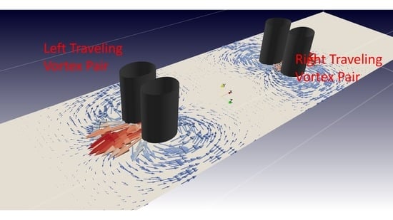
A visualization of the velocity and vorticity of the flow associated with a vortex wave obtained from the numerical simulations is shown in Figure 1A. As described above, elastic energy was released into the fluid by creating a deficit of tensile stress situated at the center of the computational domain in a small region given by and . Here, the non-dimensional and coordinates are given by and , where . As expected, this energy release creates two columnar vortex pairs with only vertical vorticity, which travel in opposite directions. Corresponding to the case shown in Figure 1, the space–time () coordinates of the maximum vertical vorticity of the left-traveling vortex pair is shown in Figure 2A. We determined that lateral () motion of the pair is negligible, indicating that the vortex pair travels almost entirely in the x-direction. We note that the vortex path shown in Figure 2A and a blow-up in Figure 2B exhibit two regions: a period of expansion, followed by one of translation. During expansion, the position of the maximum vorticity remains fixed in space, whereas during translation, its position changes.
For each numerical simulation performed in this work, we performed a linear curve fit of the path of the vorticity maximum during the translation period. In each case, the coefficient of determination () fell in the range 0.986–0.999, indicating that a linear model is an excellent approximation for the vortex paths. We therefore use the slope, , of the linear curve fit as the definition of the vortex speed in all simulations. Figure 2A shows an example of such a curve fit.
6. Linearized Wave Equation and the Undamped Solution
6.1. Linearized Wave Equation
While the results of the DNS simulations shown in Section 5 should be sufficient to verify the wave-like behavior of the vortices under consideration, it is useful to obtain further insight by examining the solutions of the linearized wave equation. In fact, it is shown that these simplified models give reasonable correspondence to the full simulations under conditions for which linearity is well approximated, and polymer relaxation times are large. In these models, we assume that the wave speed is given by the results of Section 3.
Consistent with the idea of using linearized model problems to gain further understanding of the results obtained from the DNS simulations, we consider a simplified version of Equation (21) given by
where for simplicity, the scalar field, , has been substituted for . This describes a field that propagates in one direction, , which is entirely justified by the results obtained from the full equations of motion shown in Figure 2. The inclusion of viscous damping in two ( directions is motivated by the fact that the vortices observed in the simulations shown in Figure 1 are themselves two dimensional and should be expected to diffuse in the horizontal () plane. We excluded the term in Equation (25) since we are interested in the situation with large polymer relaxation times, and we found in the cases of interest that this term has only a small effect on the decay of the vortex wave magnitude. The waves are assumed to propagate in an effectively infinite medium so no boundary conditions, except for radiation conditions, are required. We further note that damped wave equations have been investigated in the context of acoustics [77,78].
6.2. Analytical Solution for Undamped Waves
A salient aspect of the results shown in Figure 2A,B is the existence of a period of expansion followed by one of translation. Here, we show that this is entirely consistent with the solution of the undamped wave equation (Equation (25) without the damping terms) given by
In this inhomogeneous form of the wave equation, the source term on the right-hand side represents the initial conditions: the impulsive source is quiescent before being activated at time t = 0. The initial conditions for the model problem are that the initial field be zero, since the fluid is initially at rest, and that its time rate of change should be obtained from Equation (24): and
where Q represents the amplitude of the disturbance. The delta functions appearing in Equation (27) represent a model for the sharp gradients in the stress field, as described in Section 4, which result in the impulsive forces discussed in earlier work (see Figure 1 of [1]). The source strength, , in Equation (26) can be thought of as the amplitude of a force per unit mass whose spatial gradients give rise to vorticity.
The solution for the vorticity, ϕ, may be found by applying two Fourier transforms, one temporal and the other spatial, to both sides of Equation (26). After applying the appropriate inverse transforms, this procedure leads to the causal expression:
where u(t) is the Heaviside unit step function. Bearing in mind the identity
it is evident that Equation (28) is consistent with the initial condition in Equation (27).
From an elementary identity, the products of the trigonometric functions in the integrands of Equation (28) may be expressed as the sum of two sine functions:
and the integrals themselves then take the form
where sgn(X) is the signum function, with values of +1 and −1, respectively, for X > 0 and X < 0. It follows that
A schematic representation of this solution is given in Figure 3. As indicated in Figure 3B, at times such that, the field appears in the vicinity of and as two spatially narrow boxcar functions, which are designated as and , respectively. It is important to note in Figure 3B that the left and right sides of each boxcar travel in opposite directions with speed C, which results in spatially expanding fields, not translation. At time shown in Figure 3C, the fields have expanded to the maximum extent, and finally in Figure 3D, for t , the fields and propagate with a speed C to the left and right, respectively, since the sides of the boxcars propagate in the same direction. We designate the time separating expansion and translation as . The existence of a time period of wave expansion followed by a period of wave translation agrees qualitatively with the results of Figure 2A,B. We should point out that the undamped solution given here shows that the vortices travel with constant amplitudes. However, in the numerical simulations, the viscosity is not zero, and this naturally has a smoothing effect that results in a peak in the wave amplitude. It is the space–time path of this peak that is shown in Figure 2A,B. The effects of viscosity, as predicted by the linearized theory, are described below.
7. Viscous Effects
Here, we consider the effects of viscosity on the evolution of vortex waves. Recall that a good approximation for the wave speed is , in which . Thus, the wave speed itself is viscosity dependent. In addition, the viscosity of the fluids typically used in microfluidics [3] are high, resulting in low Reynolds numbers. In this section, we first present results from the numerical simulation for the evolution of the vorticity magnitude, followed by the development of analytical solutions of the linearized wave equation with damping in one and two dimensions.
7.1. Temporal Evolution of the Vorticity Magnitude from Numerical Simulations
The temporal evolution of the magnitude of the maximum vertical vorticity following a typical vortex wave is shown in Figure 4. These results were obtained from the numerical simulation described in Figure 1. Since the fluid is modeled as a solution having viscosity , it is expected that the wave energy will decay after being released. This is in fact what is observed in Figure 4A, which shows a rapid rise in vorticity followed by decay. In Figure 4B, the time taken for the vorticity to reach a maximum is compared to the transition time, . This shows that the maximum vorticity appears at a time somewhat before the transition time, which indicates the growth of wave energy lies entirely within the time scale T.
7.2. One-Dimensional Analytical Solution of the Linearized Wave Equation with Viscosity
To gain further insight into the results of the numerical simulations discussed above, an analytical solution of Equation (25) is now developed in which the effect of viscous damping on the evolution of the vortices is taken into account. Following the formalism of the undamped case in Equation (26), the one-dimensional version of Equation (25) with damping included may be written in the inhomogeneous form
where, on the left, the coefficient of the third-order derivative, representing damping, is
It is important to note that the damping coefficient, χ, is in general non-zero, thus giving rise to a smoothing of the vortex field, but χ is itself independent of the viscosity as, according to Equation (23), the vortex speed, C, scales as the square root of the viscosity, from which it follows that cancels out of Equation (34). This situation is the reverse of that associated with acoustic propagation in a viscous fluid: Stokes’ equation [77] for the acoustic field has exactly the same structure as that on the left of Equation (33), but the acoustic analogs of C and χ are, respectively, independent of and proportional to the viscosity. According to Equation (33), even though χ is invariant with , the viscosity will affect the travel time and the shape of a vortex, since C2 in the second term on the left scales with .
As with the undamped case, the solution for the vortex field may be obtained by applying a pair of Fourier transforms to Equation (33), one temporal and one spatial, as detailed in Appendix C. This procedure leads to a wave number integral for the field:
where u(t) is the Heaviside unit step function and
Bearing in mind the delta function identity in Equation (29), it is readily shown that, at the origin of time, t = 0, the time derivative of the field in Equation (35) is identical to the second of the initial conditions in Equation (27). In fact, everywhere in the medium, apart from x = ±a, the vortex field itself in Equation (35) and all of its time derivatives are identically zero at t = 0; that is to say, the field is maximally flat, or infinitely flat, at the instant the source is activated. Such behavior is also exhibited by Stokes’ equation for acoustic propagation in a viscous fluid [77] and by the time-dependent diffusion equation [77]. Thus, in all three cases, the field satisfies causality in the strict sense: it is zero at negative times with no instantaneous arrivals anywhere in the fluid medium surrounding the source.
The function R in Equation (36) is real when and imaginary when , where
For all practical values of χ, the contribution to the integral in Equation (35) from the imaginary components of R is negligible, and for R real, an excellent approximation is
Under these conditions, the integral in Equation (35) may be approximated in terms of the error function, erf(.), as shown in Appendix C:
where sgn(.) is the signum function taking values of +1 and −1, respectively, for positive and negative arguments. A simple normalization scheme has been introduced in Equation (39), whereby
The factor of ½ in each of the four terms in Equation (39) ensures that, in the absence of damping, when χ = 0, the peak value of the normalized vortex field is . It is worth noting that when χ = 0, the error functions in Equation (39) are all unity, and the field reduces to precisely the same rectangular boxcar form as that of the undamped solution in Equation (32). The normalization scheme in Equation (40) can also be applied to the exact integral solution in Equation (35), in which case the normalized vorticity field becomes
where
An advantage of the normalization in Equations (39) and (41) is that the wave speed C in which the viscosity is embedded, the damping coefficient , and the source positions at |x| = a, all collapse into the single parameter, , which, through the presence of C, varies as the inverse square root of the viscosity. Bearing in mind that the normalizing terms χ and a in the denominators of Equation (40) are independent of ν0, it is evident that the effects of viscosity on the normalized vortex field in Equations (39) and (40) are represented solely by the dimensionless parameter qa. Therefore, with a fixed receiver position, , a family of curves for as a function of may be generated in which each curve corresponds to a particular value of qa, with lower values of qa representing higher viscosities. Two such families of curves, for and , are shown in Figure 5 (N.B. the logarithmic time scale).
These curves were computed by numerical evaluation of the integrals in Equation (40), but the error function approximation in Equation (39) could have been used since it returns almost identical results for viscosities represented by the condition qa ≥ 10. For smaller values of qa, corresponding to inordinately high viscosities, the error function approximation in Equation (39) becomes increasingly inaccurate, and instead, the exact integral formulation in Equation (41) is recommended. Three effects of increasing the viscosity are illustrated by the vorticity fields shown in Figure 5: the travel time is progressively reduced, consistent with the scaling of the wave speed as the square root of the viscosity; the rectangular boxcar shape characteristic of low viscosities becomes more rounded; and the maximum level of the normalized vortex field is reduced.
7.3. Two-Dimensional Analytical Solution of the Linearized Wave Equation with Viscosity
It was found through comparison of the simulations with the analytical model described above that wave damping in one dimension gives wave amplitudes that decay more slowly than indicated by the numerical simulations. To gain further insight into the viscous decay of the vortex, the wave equation in Equation (25), may be written in inhomogeneous form as
where
Note that damping terms in and are added (third term on the left-hand side of Equation (43)). The solution to Equation (43) is given in Appendix D.
Here, we are particularly interested in the rate of decay of the vorticity, which is evident in Figure 4 for . It is reasonable to approximate this decay as an exponential of the form to model the evolution of both the vorticity obtained from the numerical simulations and the analytical solution, Equation (A25), which has been evaluated numerically. The results for the numerical simulations shown in Figure 4 and the model (Equation (43)) are and 0.732 where , where the coefficients of determination () for the exponential model were and , respectively. The satisfactory agreement for the decay rates indicates that the decay in the vorticity of the vortex wave can be accounted for reasonably well by viscous diffusion in two dimensions. It is also notable that the decay time, , for the vortex wave is , as expected from dimensional considerations, since the size of the vortex is on the order of .
8. Vortex Wave Speed
Here, numerical simulations are used to determine the effects of wave amplitude, the initial elastic stress in the fluid, and the maximum polymer extension length on the speed of vortex waves. The results below show excellent agreement between the linearized theory discussed in Section 3 and provide strong evidence for the existence of vortex waves.
8.1. Effect of Wave Amplitude on Wave Speed
The full equations of motion (1)–(6) contain nonlinearities, such as advection, vortex stretching and tilting, and polymer stretching, which are fully represented in all numerical simulations presented in this work. The effects of these nonlinearities on wave motion can be important for waves of high amplitude [70]. For example, acoustic waves can be characterized by the ratio , where is the amplitude of the wave and is the ambient atmospheric pressure. When an acoustic wave passes a given location, the perturbation in the pressure, , is normally observed by acoustic sensors. When << 1, acoustic waves have a well-known speed given by , where is the ratio of specific heats and is the ambient air density. However, acoustic waves of high amplitude (e.g., shock waves) can have speeds higher than . Moreover, high amplitude nonlinear waves can exhibit other effects, such as wave steepening, and dispersion (e.g., ocean waves).
It is therefore of interest to determine the effects of wave amplitude on the propagation of vortex waves. This was achieved by performing numerical simulations in which the fluid properties were fixed and using the linear spring model, , while varying the amplitude parameter , the ratio of the initial stress deficit to the background stress, by more than an order of magnitude. Here, can thought of as analogous to for acoustic waves. Here, we define (see Section 3) the theoretical wave speed by.
The results shown in Figure 6 indicate that the wave speed is virtually unaffected by the wave amplitude. In addition, the difference between the wave speeds obtained from the simulations shown in Figure 6 and the theoretical linear wave speed was <1.5% in all cases. This indicates that, over a significant range of wave amplitude, a linear wave model is a good approximation for the observed dynamics.
8.2. Effect of the Initial Elastic Stress on Wave Speed
The dependence of wave speed on for the linear spring model is shown in Figure 7. In these simulations, all fluid properties were fixed and , thus ensuring linearity. These results show clearly that the wave speeds predicted by the linearized model are in excellent agreement with the numerical simulations. In fact, the difference between the wave speeds obtained from the simulations shown in Figure 7 and the theoretical linear wave speeds was <1.1% in all cases. As further evidence for the accuracy of the linearized theory of vortex waves, we show in Figure 2C the relation between the transition time, , and for both simulations and theory. The agreement is again quite reasonable and further justifies the model given in Section 6.2. Furthermore, it indicates that for the kind of initial conditions we imposed on the flow, a reasonable estimate of the vortex wave speed can be obtained from T and the length scale .
8.3. Effect of the Maximum Polymer Extensional Length on Wave Speed
It is also of interest to determine the effect of a nonlinear spring on vortex wave speed by allowing the spring constant in the polymer model to be determined by the Peterlin function . Here, we note that as the maximal allowable polymer extensional length () becomes large compared to . In this limit, it is expected that the wave speed should approach the linear theory limit. To test this, wave speeds were determined aswas varied over two orders of magnitude, with all other fluid and polymer properties fixed, and with during the course of the simulations. The results shown in Figure 8 indicate that at the largest value of , wave speeds approach nearly the theoretical speed for linear waves. However, as decreases, the Peterlin function increases, corresponding to an increasingly stiff spring. The effect of this is to increase vortex wave speed, an expected result that is clearly indicated in Figure 8. It should also be noted that in every case, the vortex wave speed is greater than the linear theory wave speed for these nonlinear springs.
9. Summary and Discussion
Recent work [1] has shown that the release of elastic energy in a viscoelastic fluid can produce coherent vorticity, which is generated by torque-producing elastic stress gradients. However, in that work, the kinematics of the motion of the coherent vortical structures was not fully explored. In this work, we show that the release of elastic energy generates vorticity that propagates as a wave, whose speed is governed by the initial stress field in the fluid. A linearized version of the equations of motion for an incompressible fluid, which includes the FENE-P model for polymer dynamics, shows that waves of vorticity should be generated upon release of stored elastic energy. For large polymer relaxation times and for a linear spring model (), the vortex wave speed is shown to be , where is the initial longitudinal polymer conformation, proportional to the initial tension in the fluid. Furthermore, the theory shows that the wave should be affected by the fluid viscosity. Insight was obtained by using an undamped model for the case in which energy is released in a spatially symmetric manner. This shows that the temporal evolution of the wave takes place in two parts: (1) a period of expansion in which the field grows in spatial extent but does not propagate, followed by (2) a field which propagates at speed . The period of expansion is shown to take place during a time , where is the spatial location at which energy is released, and also represents the length scale or size of the wave. In addition, an analytical solution to the linearized equations with viscous damping was used to determine a viscous decay time scale.
Analogous to physical experiments, a series of direct numerical simulations (DNS) were performed for a range of parameters that could be compared with the theory. For low amplitude waves that are governed by a linear spring model, the DNS gave results very much in accord with the linearized theory: (1) wave speeds obtained from DNS were within 1.5% of the theory, and (2) the time scale associated with the period of wave expansion matched DNS results. In addition, an analytical solution of the wave equation with viscous damping was used to determine a viscous decay time scale. This time scale was in good agreement with DNS results.
An additional motivation for undertaking this work is associated with the problem of promoting mixing in low Reynolds flows, such as those associated with microfluidics. As such, coherent vortex motions may be useful for the enhancement of transport in low Reynolds number, high Peclet number flows in micro-devices. The possibility of experimentally verifying the phenomena described in this work is also being pursued. For example, recent experiments [79] in which an extensional flow of a dilute polymer solution using a convergent–divergent flow field revealed chaotic flow behavior. If stored elastic energy in such a flow could be released in a controlled manner, then fluid motions similar to the ones observed in our simulations should be generated. It is also interesting to observe that vortex waves can easily be made to propagate in any desired direction. For example, if stored elastic energy placed in is suddenly released, we should expect the resultant vortex waves to propagate in the vertical direction, perpendicular to walls. Future work should also consider the effects of an initially asymmetric stress distribution, as well as the effects of strong, finite amplitude waves.
Author Contributions
Conceptualization, R.A.H. and M.J.B.; methodology, R.A.H. and M.J.B.; software, R.A.H. and M.J.B.; validation, R.A.H. and M.J.B.; formal analysis, R.A.H. and M.J.B.; investigation, R.A.H. and M.J.B.; resources, R.A.H. and M.J.B.; data curation, R.A.H. and M.J.B.; writing—original draft preparation, R.A.H. and M.J.B.; writing—review and editing, R.A.H. and M.J.B.; visualization, R.A.H. and M.J.B.; supervision, R.A.H. and M.J.B.; project administration, R.A.H. and M.J.B.; funding acquisition, R.A.H. and M.J.B. All authors have read and agreed to the published version of the manuscript.
Funding
This research was funded by the National Science Foundation under grant number 1904953 and by the Office of Naval Research under grant number N000141812126.
Institutional Review Board Statement
Not applicable.
Informed Consent Statement
Not applicable.
Data Availability Statement
Not applicable.
Acknowledgments
Simulations were performed on ARGO, a research computing cluster provided by the Office of Research Computing at George Mason University.
Conflicts of Interest
The authors have no conflict of interest.
Appendix A. Derivation of the Initial Time Rate of Change of the Vorticity
Here, we give further details regarding the derivation of Equation (7), which relates the initial time rate of change of vorticity to spatial gradients of the elastic stresses. Refer to the text or Table A1 in Appendix B for the definitions of all symbols not explicitly defined in this Appendix. Two assumptions are made in this derivation: (1) the fluid velocity at time , and (2) the maximal allowable polymer length is assumed to be such that so that is a constant. We note that since the fluid velocity is initially zero everywhere in the fluid, then the vorticity is also zero at .
For convenience, we rewrite the evolution equation for the vorticity (Equation (6)):
The first term on the left-hand side of Equation (A1), which represents the material derivative of the vorticity, can be written using index notation in Cartesian coordinates as follows:
where , and repeated indices imply summation. Evaluation of Equation (A2) at and using assumption (1) above gives
since the second term on the right-hand side of Equation (A2) vanishes. The first and second terms on the right-hand side of Equation (A1) also vanish because of assumption (1). Since the polymer stress is given by
the third term on the right-hand side of Equation (A1) can be written as
where is the permutation symbol, and is a unit vector. However, since both and are constants, Equation (A1) becomes
where both sides are evaluated at . This corresponds exactly to Equation (7) in the text. We note that Equation (A6) states that although the initial vorticity is zero, the initial time rate of change of vorticity is not zero when elastic stress gradients are initially present in the fluid.
Appendix B. Table of Symbols

Table A1.
This table lists all relevant symbols used in this work. For each symbol, a definition is given followed by a designation of the symbol as dimensional (e.g., centimeters, seconds) or dimensionless.
Table A1.
This table lists all relevant symbols used in this work. For each symbol, a definition is given followed by a designation of the symbol as dimensional (e.g., centimeters, seconds) or dimensionless.
| Symbol | Definition | Units |
|---|---|---|
| Coordinates: the vortex waves travel in the x-direction, z is perpendicular to this direction, and y is the vertical direction (see Figure 1) | Dimensional | |
| Scripted coordinates corresponding to | Dimensional | |
| Lengths of the computational domain in the , , and directions. is the half-height of the computational domain in the y-direction | Dimensional | |
| Coordinates x,y,z made dimensionless using | Dimensionless | |
| Computational domain lengths made dimensionless using . Note that this definition leads to . | Dimensionless | |
| Time | Dimensional | |
| Velocity and components of the velocity | Dimensional | |
| Vorticity and components of the vorticity | Dimensional | |
| Polymer conformation tensor and its components | Dimensionless. The conformation tensor is made dimensionless using the rest length of the polymer molecule | |
| Fluid pressure | Dimensional | |
| Average or mean value of the velocity (e.g., time or ensemble averaged) and its perturbation | Dimensional | |
| Average or mean value of the vorticity (e.g., time or ensemble averaged) and its perturbation | Dimensional | |
| Average or mean value of the conformation tensor (e.g., time or ensemble averaged) and its perturbation | Dimensional | |
| Average or mean value of the pressure (e.g., time or ensemble averaged) and its perturbation | Dimensional | |
| Solution viscosity | Dimensional | |
| Polymer relaxation time | Dimensional | |
| Ratio of the solvent to the solution viscosity | Dimensionless | |
| Stress parameter. | Dimensional | |
| Maximum possible extensional length made dimensionless using the polymer rest length | Dimensionless | |
| Vortex wave speed. See definition directly following Equation (21). | Dimensional | |
| Length associated with the region in which the fluid tension experiences a deficit. The region is a square with length on each side. See Figure 1B. | Dimensional | |
In the simulations and theory, . See Figure 1B. | Dimensionless | |
| The transition time a/C. Before this time, the vortex wave expands without translating. Translation occurs when | Dimensional | |
| Dimensionless transition time, . | Dimensionless | |
| Dimensionless time. = . | Dimensionless | |
| Dimensionless vortex wave speed.. | Dimensionless | |
| Initial value of the component of the conformation tensor, which is directly proportional to the fluid tension in the fluid. | Dimensionless | |
| The Peterlin function. where . | Dimensionless | |
| Amplitude of the polymer conformation deficit, which is proportional to the stress deficit. | Dimensionless | |
| Amplitude parameter given by . When , the vortex wave can be considered linear. | Dimensionless | |
| Component of the vorticity in the vertical (y) direction. | Dimensional | |
| Dimensionless vertical vorticity where . | Dimensionless | |
| translational time scale for a vortex wave | Dimensional | |
| d | distance traveled by a vortex wave in time | Dimensional |
| Q | amplitude of the source of the vortex wave | Dimensional |
Appendix C. Analytical Solution of the One-Dimensional Damped, Linearized Vorticity Equation
Equation (33) in the text is the one-dimensional, inhomogeneous equation to be solved for the scalar vorticity field, ϕ = ϕ(x,t):
Taking the Fourier transform with respect to time returns
where
A further Fourier transform, with respect to x, yields
where p is the wavenumber and
From Equation (A10), the solution for the doubly transformed field is
which has two poles in the complex ω-plane at
where
Since p is real, both poles lie in the upper half-plane. Taking the inverse Fourier transform of Equation (A12) with respect to ω, it follows that, for t < 0, an integration around a D-contour in the lower half-plane returns zero, indicating that the vortex field is causal in that there are no arrivals prior to t = 0. For t > 0, from Jordan’s lemma and Cauchy’s theorem, an integration around a D-contour in the upper half-plane yields
where u(t) is the Heaviside unit step function. The inverse Fourier transform of Equation (A15) with respect to p leads to the following wavenumber integral for the field:
which is the solution that is presented in Equation (35) in the text. An extension to two dimensions may be obtained by following a similar procedure but with two spatial Fourier transforms applied to the wave equation, which leads to a double wavenumber integral for the vortex field.
An approximation for the integral in Equation (A16) may be obtained by neglecting the fourth-order term in the radical in the expression for R in Equation (A14), under which condition
The expression for the field then becomes
The product of the three sine functions in the integrand can be expressed as the sum of four sine functions of the form
where all four combinations of the plus and minus signs are to be taken. This gives rise to four Fourier sine transforms, which can be found in Tables of Integrals:
This result leads to the final approximate expression for the vortex field,
where the superscript and subscript notation has been introduced to define the signs in the expressions for X, for example,
After normalization, the approximate error function solution in Equation (A21) becomes identical to that in Equation (39) in the main text.
Appendix D. Analytical Solution of the Two-Dimensional Damped, Linearized Vorticity Equation
The solution to Equation (43) in the main text is obtained by applying three Fourier transforms, one temporal and two spatial, and then to perform the inverse transforms, which leads to the formulation of the field in terms of a double wave number integral. Taking the transform variables (wave numbers) in x and z as p and q, respectively, the solution for the field in double wave number space is
where
On the left of Equation (A23), we used the convention that a subscript denotes a spatial Fourier transform, which is of course a function of the transform variable in question (p or q in the present case). The field itself is obtained by applying the two inverse spatial Fourier transforms to Equation (A23), yielding
Equation (A25) was evaluated numerically, noting that two regions exist, given by
References
- Handler, R.A.; Blaisten-Barojas, E.; Ligrani, P.M.; Dong, P.; Paige, M. Vortex generation in a finitely extensible nonlinear elastic Peterlin fluid initially at rest. Eng. Rep. 2020, 2, e12135. [Google Scholar] [CrossRef] [Green Version]
- Pan, L.; Morozov, A.; Wagner, C.; Arratia, P.E. Nonlinear Elastic Instability in Channel Flows at Low Reynolds Numbers. Phys. Rev. Lett. 2013, 110, 174502. [Google Scholar] [CrossRef]
- Qin, B.; Arratia, P.E. Characterizing elastic turbulence in channel flows at low Reynolds number. Phys. Rev. Fluids 2017, 2, 083302. [Google Scholar] [CrossRef]
- Kim, K.; Adrian, R.J.; Balachandar, S.; Sureshkumar, R. Dynamics of Hairpin Vortices and Polymer-Induced Turbulent Drag Reduction. Phys. Rev. Lett. 2008, 100, 134504. [Google Scholar] [CrossRef] [Green Version]
- Kim, K.; Sureshkumar, R. Spatiotemporal evolution of hairpin eddies, Reynolds stress, and polymer torque in polymer drag-reduced turbulent channel flows. Phys. Rev. E 2013, 87, 063002. [Google Scholar] [CrossRef] [Green Version]
- Min, T.; Yoo, J.Y.; Choi, H.; Joseph, D.D. Drag reduction by polymer additives in a turbulent channel flow. J. Fluid Mech. 2003, 486, 213–238. [Google Scholar] [CrossRef] [Green Version]
- Toms, B.A. Some observations on the flow of linear polymer solutions straight tubes at large Reynolds numbers. In Proceedings of the International Congress on Rheology; North Holland: Amsterdam, The Netherlands, 1948; Volume 2, pp. 135–141. [Google Scholar]
- Samantha, G.; Housiadis, K.D.; Handler, R.A.; Beris, A.N. Effects of viscoelasticity on the probability density functions in turbulent channel flow. Phys. Fluids 2009, 21, 115106. [Google Scholar] [CrossRef]
- White, C.M.; Mungal, M.G. Mechanics and prediction of turulent drag reduction with polymer additives. Annu. Rev. Fluid Mech. 2008, 40, 235–256. [Google Scholar] [CrossRef]
- Lumley, J.L. Drag reduction by additives. Annu. Rev. Fluid Mech. 1969, 1, 367–384. [Google Scholar] [CrossRef]
- Sureshkumar, R.; Beris, A.N.; Handler, R.A. Direct numerical simulation of the turbulent channel flow of a polymer solution. Phys. Fluids 1997, 9, 743–755. [Google Scholar] [CrossRef]
- Dimitropoulos, C.D.; Sureshkumar, R.; Beris, A.N. Direct numerical simulation of viscoelastic turbulent channel flow exhibiting drag reduction: Effect of the variation of rheological parameters. J. Non-Newton. Fluid Mech. 1998, 79, 433–468. [Google Scholar] [CrossRef]
- Dimitropoulos, C.D.; Sureshkumar, R.; Beris, A.N.; Handler, R.A. Budgets of Reynolds stress, kinetic energy and streamwise enstrophy in viscoelastic turbulent channel flow. Phys. Fluids 2001, 13, 1016–1027. [Google Scholar] [CrossRef]
- Housiadas, K.; Beris, A.N.; Handler, R.A. Viscoelastic effects on higher order statistics and on coherent structures in turbulent channel flow. Phys. Fluids 2005, 17, 35106. [Google Scholar] [CrossRef]
- Handler, R.A.; Housiadas, K.; Beris, A.N. Karhunen–Loeve representations of turbulent channel flows using the method of snapshots. Int. J. Numer. Methods Fluids 2006, 52, 1339–1360. [Google Scholar] [CrossRef]
- Virk, P.S. Drag reduction fundamentals. AIChE J. 1975, 21, 625–656. [Google Scholar] [CrossRef]
- De Gennes, P. Towards a scaling theory of drag reduction. Physica A 1986, 140, 9–25. [Google Scholar] [CrossRef]
- Manz, A.; Harrison, D.J.; Verpoorte, E.; Widmer, H.M. Planar chips technology for miniaturization of separation systems: A developing perspective in chemical monitoring. Adv. Chromatogr. 1993, 33, 1–66. [Google Scholar]
- Reyes, D.R.; Iossifidis, D.; Auroux, P.A.; Manz, A. Micro total analysis systems. Introduction, theory, and technology. Anal. Chem. 2002, 74, 2623–2636. [Google Scholar]
- Vijayendran, R.A.; Motsegood, K.M.; Beebe, D.J.; Leckband, D.E. Evaluation of a three-dimensional micromixer in a surface-based biosensor. Langmuir 2003, 19, 1824–1828. [Google Scholar] [CrossRef]
- Ho, C.M.; Tai, Y.C. Micro-electro-mechanical-systems (MEMS). Annu. Rev. Fluid Mech. 1998, 30, 579–612. [Google Scholar] [CrossRef] [Green Version]
- Verpoorte, E.; De Rooij, N.F. Microfluidics meets MEMS. Proc. IEEE 2003, 91, 930–953. [Google Scholar] [CrossRef] [Green Version]
- Wiggins, S.; Ottino, J.M. Foundations of chaotic mixing. Philos. Trans. R. Soc. A 2004, 362, 937–970. [Google Scholar] [CrossRef]
- Eckart, C. An analysis of the stirring and mixing processes in incompressible fluids. J. Mar. Res. 1948, 7, 265–275. [Google Scholar]
- Aref, H.; Balachandar, S. Chaotic advection in a Stokes flow. Phys. Fluids 1986, 29, 3515. [Google Scholar] [CrossRef]
- Ottino, J.M. The Kinematics of Mixing: Stretching, Chaos, and Transport; Cambridge University Press: Cambridge, UK, 1989. [Google Scholar]
- Stremler, M.A.; Haselton, F.R.; Aref, H. Designing for chaos: Applications of chaotic advection at the microscale. Philos. Trans. R. Soc. A 2004, 362, 1019–1036. [Google Scholar] [CrossRef] [PubMed]
- Bringer, M.R.; Gerdts, C.J.; Song, H.; Tice, J.D.; Ismagilov, R.F. Microfluidic systems for chemical kinetics that rely on chaotic mixing in droplets. Philos. Trans. R. Soc. A 2004, 362, 1087–1104. [Google Scholar] [CrossRef] [Green Version]
- Bottausci, F.; Mezic, I.; Meinhart, C.D.; C. Cardonne, C. Mixing in the shear superposition micromixer: Three dimensional analysis. Philos. Trans. R. Soc. A 2004, 362, 1001–1008. [Google Scholar] [CrossRef] [PubMed]
- Campbell, C.J.; Grzybowski, B.A. Microfluidic Mixers: From Microfabricated to Self-Assembled Devices. Philos. Trans. R. Soc. A 2004, 362, 1069–1086. [Google Scholar] [CrossRef] [PubMed]
- Darhuber, A.A.; Chen, J.Z.; Davis, J.M.; Troian, S.M. A study of mixing in thermocapillary flows on micropatterned surfaces. Philos. Trans. R. Soc. A 2004, 362, 1037–1058. [Google Scholar] [CrossRef] [PubMed]
- Mensing, G.A.; Pearce, T.M.; Graham, M.D.; Beebe, D.J. An externally driven magnetic microstirrer. Philos. Trans. R. Soc. A 2004, 362, 1059–1068. [Google Scholar] [CrossRef] [PubMed]
- Stroock, A.D.; McGraw, G.J. Investigation of the staggered herringbone mixer with a simple analytical model. Philos. Trans. R. Soc. A 2004, 362, 971–986. [Google Scholar] [CrossRef] [PubMed]
- Tabeling, P.; Chabert, M.; Dodge, A.; Jullien, C.; Okkels, F. Chaotic mixing in cross-channel micromixers. Philos. Trans. R. Soc. A 2004, 362, 987–1000. [Google Scholar] [CrossRef] [PubMed]
- Stroock, A.; Dertinger, S.K.W.; Ajdari, A.; Mezić, I.; Stone, H.A.; Whitesides, G.M. Chaotic Mixer for Microchannels. Science 2002, 295, 647–651. [Google Scholar] [CrossRef] [PubMed] [Green Version]
- Ottino, J.M. Mixing, chaotic advection and turbulence. Annu. Rev. Fluid Mech. 1990, 22, 207–253. [Google Scholar] [CrossRef]
- Aref, H. Stirring by chaotic advection. J. Fluid Mech. 1984, 143, 1–23. [Google Scholar] [CrossRef]
- Chou, H.-P.; Unger, M.A.; Quake, S.R. A Microfabricated Rotary Pump. Biomed. Microdevices 2001, 3, 323–330. [Google Scholar] [CrossRef]
- Sudarsan, A.P.; Ugaz, V.M. Multivortex micromixing. Proc. Natl. Acad. Sci. USA 2006, 103, 7228–7233. [Google Scholar] [CrossRef] [PubMed] [Green Version]
- Xia, S.; Wan, Y.M.; Shu, C.; Chew, Y.T. Chaotic micromixers using two-layer crossing channels to exhibit fast mixing at low Reynolds numbers. Lab. Chip 2005, 5, 748–755. [Google Scholar] [CrossRef]
- Nguyen, N.; Wu, Z. Micromixers—A review. J. Micromech. Microeng. 2005, 15, R1–R16. [Google Scholar] [CrossRef]
- Bau, H.H.; Zhong, J.; Yi, M. A minute magnetohydrodynamic (MHD) mixer. Sens. Actuators B 2001, 79, 207–215. [Google Scholar] [CrossRef] [Green Version]
- Mao, H.; Yang, T.; Cremer, P.S. A microfluidic device with a linear temperature gradient for parallel and combinatorial measurements. J. Am. Chem. Soc. 2002, 124, 4432–4435. [Google Scholar] [CrossRef] [PubMed]
- Tsai, J.H.; Lin, L. Active microfluidic mixer and gas bubble filter driven by thermal bubble pump. Sens. Actuators A 2002, 97–98, 665–671. [Google Scholar] [CrossRef]
- Liu, R.H.; Yang, J.; Pindera, M.Z.; Athavale, M.; Grodzinski, P. Bubble-induced acoustic micromixing. Lab. Chip 2002, 2, 151–157. [Google Scholar] [CrossRef]
- Liu, R.H.; Lenigk, R.; Druyor-Sanchez, R.L.; Yang, J.; Grodzinski, P. Hybridization Enhancement Using Cavitation Microstreaming. Anal. Chem. 2003, 75, 1911–1917. [Google Scholar] [CrossRef] [PubMed]
- Yaralioglu, G.G.; Wygant, I.O.; Marentis, T.C.; Khuri-Yakub, B.T. Ultrasonic mixing in microfluidic channels using integrated transducers. Anal. Chem. 2004, 76, 3694–3698. [Google Scholar] [CrossRef]
- Squires, T.M.; Quake, S.R. Microfluidics: Fluid physics at the nanoliter scale. Rev. Mod. Phys. 2005, 77, 977–1025. [Google Scholar] [CrossRef] [Green Version]
- Stone, H.A.; Stroock, A.D.; Ajdari, A. Engineering flows in small devices: Microfluidics toward a Lab-on-a-Chip. Annu. Rev. Fluid Mech. 2004, 36, 381–411. [Google Scholar] [CrossRef] [Green Version]
- Pearson, J.R.A. Instability in Non-Newtonian Flow. Annu. Rev. Fluid Mech. 1976, 8, 163–181. [Google Scholar] [CrossRef]
- Petrie, C.J.S.; Denn, M.M. Instabilities in polymer processing. AIChE J. 1976, 22, 209–236. [Google Scholar] [CrossRef]
- Larson, R.G. Instabilities in viscoelastic flows. Rheol. Acta 1992, 31, 213–263. [Google Scholar] [CrossRef]
- McKinley, G.; Pakdel, P.; Öztekin, A. Rheological and geometric scaling of purely elastic flow instabilities. J. Non-Newton. Fluid Mech. 1996, 67, 19–47. [Google Scholar] [CrossRef]
- Baumert, B.M.; Muller, S.J. Flow visualization of the elastic Taylor-Couette instability in Boger fluids. Rheol. Acta 1995, 34, 147–159. [Google Scholar] [CrossRef]
- Graham, M. Effect of axial flow on viscoelastic Taylor–Couette instability. J. Fluid Mech. 1998, 360, 341–374. [Google Scholar] [CrossRef]
- Pakdel, P.; McKinley, G. Elastic Instability and Curved Streamlines. Phys. Rev. Lett. 1996, 77, 2459–2462. [Google Scholar] [CrossRef]
- Phan-Thien, N. Coaxial-disk flow of an Oldroyd-B fluid: Exact solution and stability. J. Non-Newton. Fluid Mech. 1983, 13, 325–340. [Google Scholar] [CrossRef]
- Phan-Thien, N. Cone-and-plate flow of the Oldroyd-B fluid is unstable. J. Non-Newton. Fluid Mech. 1985, 17, 37–44. [Google Scholar] [CrossRef]
- McKinley, G.H.; Byars, J.A.; Brown, R.A.; Armstrong, R.C. Observations on the elastic instability in cone-and-plate and parallel-plate flows of a polyisobutylene Boger fluid. J. Non-Newton. Fluid Mech. 1991, 40, 201–229. [Google Scholar] [CrossRef]
- McKinley, G.; Öztekin, A.; Byars, J.A.; Brown, R.A. Self-similar spiral instabilities in elastic flows between a cone and a plate. J. Fluid Mech. 1995, 285, 123–164. [Google Scholar] [CrossRef]
- Byars, J.A.; Öztekin, A.; Brown, R.A.; McKinley, G. Spiral instabilities in the flow of highly elastic fluids between rotating parallel disks. J. Fluid Mech. 1994, 271, 173–218. [Google Scholar] [CrossRef]
- McKinley, G.H.; Armstrong, R.C.; Brown, R.A. The wake instability in viscoelastic flow past confined circular cylinders. Philos. Trans. R. Soc. A 1993, 344, 265–304. [Google Scholar]
- Graham, M.D. Iterfacial hoop stress and instability of viscoelastic free surface flows. Phys. Fluids 2003, 15, 1702–1710. [Google Scholar] [CrossRef] [Green Version]
- Kumar, K.A.; Graham, M.D. Bckling instabilities in models of viscoelastic free surface flows. J. Non-Newton. Fluid Mech. 2000, 89, 337–351. [Google Scholar] [CrossRef]
- Ligrani, P.M.; Copeland, D.; Ren, C.; Su, M.; Suzuki, M. Het transfer enhancements from elastic turbulence using sucrose-based polymer solutions. AIAA J. Thermophys. Heat Transf. 2018, 32, 51–60. [Google Scholar] [CrossRef] [Green Version]
- Ligrani, P.M.; Su, M.; Pippert, A.; Handler, R.A. Thermal Transport of Viscoelastic Fluids Within Rotating Couette Flows. J. Thermophys. Heat Transf. 2020, 34, 121–133. [Google Scholar] [CrossRef]
- Bird, R.B.; Curtiss, C.F.; Armstrong, R.C.; Hassager, O. Dynamics of Polymeric Liquids Kinetic Theory, 2nd ed.; John Wiley & Sons: New York, NY, USA, 1987; Volume 2. [Google Scholar]
- Tanner, R.I. Engineering Rheology; Oxford University Press: Oxford, UK, 2002. [Google Scholar]
- Ghosh, I.; McKinley, G.; Brown, R.A.; Armstrongb, R.C. Deficiencies of FENE dumbbell models in describing the rapid stretching of dilute polymer solutions. J. Rheol. 2001, 45, 721–758. [Google Scholar] [CrossRef] [Green Version]
- Morse, P.M.; Ingard, K.U. Theoretical Acoustics; McGraw-Hill: New York, NY, USA, 1968. [Google Scholar]
- Vajipeyajula, B.; Khambampati, T.; Handler, R.A. Dynamics of a single buoyant plume in a FENE-P fluid. Phys. Fluids 2017, 29, 091701. [Google Scholar] [CrossRef]
- Canuto, C.; Hussaini, M.Y.; Quarteroni, A.; Zang, T.A. Spectral Methods in Fluid Dynamics; Springer: Berlin, Germany, 1998. [Google Scholar]
- Kim, J.; Moin, P.; Moser, R. Turbulence statistics in fully developed channel flow at low Reynolds number. J. Fluid Mech. 1987, 177, 133–166. [Google Scholar] [CrossRef] [Green Version]
- Swearingen, J.D.; Crouch, J.D.; Handler, R.A. Dynamics and stability of a vortex ring impacting a solid boundary. J. Fluid Mech. 1995, 297, 1–28. [Google Scholar] [CrossRef]
- McCormack, P.D.; Crane, L. Physical Fluid Dynamics; Academic Press: New York, NY, USA, 1973. [Google Scholar]
- Richter, D.; Iaccarino, G.; Shaqfeh, E.S.G. Simulations of three-dimensional viscoelastic flows past a circular cylinder at moderate Reynolds numbers. J. Fluid Mech. 2010, 651, 415–442. [Google Scholar] [CrossRef] [Green Version]
- Buckingham, M.J. Causality, Stokes’ wave equation, and acoustic pulse propagation in a viscous fluid. Phys. Rev. E 2005, 72, 026610. [Google Scholar] [CrossRef] [PubMed] [Green Version]
- Gaunaurd, G.C.; Everstine, G.C. Viscosity Effects on the Propagation of Acoustic Transients. J. Vib. Acoust. 2001, 124, 19–25. [Google Scholar] [CrossRef]
- Sousa, P.C.; Pinho, F.T.; Alves, M.A. Purely-elastic flow instabilities and elastic turbulence in microfluidic cross-slot devices. Soft Matter 2018, 14, 1344–1354. [Google Scholar] [CrossRef] [PubMed] [Green Version]
Figure 1.
(A) Snapshot of two columnar vortex pairs traveling in opposite directions obtained from a direct numerical simulation. The flow is shown at
where
=
is a non-dimensional time. The domain lengths in the
and
directions, normalized by the channel half-height, were
and
. The entire domain is shown in the image. The vortex wave system is generated at x =
, where
= 0.25. The image shown is from a simulation in which
=
, and
. The vortex system is visualized using an iso-surface of the vertical vorticity,
where
. Velocity vectors on the central plane are also shown, where velocity is made non-dimensional by
. In all figures, the same non-dimensional variables are used, along with
to define the non-dimensional
coordinate. In this image, all coordinates are made non-dimensional in the same way; (B) Schematic (not drawn to scale) showing the location of the region of stress deficit relative to the computational domain. The
plane is shown in which the region of stress deficit is located within a box whose sides are of length
where
= 0.25. The center of the box is located at the exact center of the computational domain. Arrows indicate the direction of translation of the vortices produced by the release of elastic energy, and red arrows indicate the sense of vortex rotation. The y-direction is directed outward perpendicular to the plane of the paper. Refer to Table A1 in Appendix B for further definitions of these length scales.

Figure 2.
Space–time diagrams (A,B) of the path of maximum vertical vorticity associated with the left-traveling vortex pair shown in Figure 1A. In (A,B), simulation results are given by filled triangles, and a linear curve fit ( is given by filled circles. In (B), regions of expansion and translation are shown. In (C), the transition time is shown () designates linear theory and filled triangles are used for the simulation results as a function of for cases in which and .

Figure 3.
Schematic representations of the wave field at three different times (B–D) generated from an undamped wave model given the forcing function see (A). The time periods corresponding to (B–D) are, respectively, and The field is an exact solution of the one-dimensional wave equation with initial conditions given by Equation (27). The wave field has two components and , which are shown during the expansion period (B,C) and during the translation period (D). Note that in (D), the left and right sides of the boxcars travel in the same direction. Here, is the point of origin of the field, and C is the wave speed.


Figure 4.
Temporal evolution (A) of the maximum vertical vorticity for the simulation shown in Figure 1. In (B), the time at which the vorticity peaks (filled triangles) is compared to the transition time obtained from the linear theory ().
Figure 4.
Temporal evolution (A) of the maximum vertical vorticity for the simulation shown in Figure 1. In (B), the time at which the vorticity peaks (filled triangles) is compared to the transition time obtained from the linear theory ().

Figure 5.
Temporal evolution of the vorticity for a one-dimensional damped wave showing the transition from a weakly damped () to a strongly damped () wave obtained from the approximate solution to Equation (39). The wave amplitude is shown for (A) and (B).
Figure 5.
Temporal evolution of the vorticity for a one-dimensional damped wave showing the transition from a weakly damped () to a strongly damped () wave obtained from the approximate solution to Equation (39). The wave amplitude is shown for (A) and (B).


Figure 6.
Dependence of the vortex wave speed on the amplitude parameter N for which = 2.4 and . Here and in subsequent figures, the theoretical wave speed is given by . Linear theory is designated by , and simulation results are given by filled triangles.
Figure 6.
Dependence of the vortex wave speed on the amplitude parameter N for which = 2.4 and . Here and in subsequent figures, the theoretical wave speed is given by . Linear theory is designated by , and simulation results are given by filled triangles.

Figure 7.
Dependence of the vortex wave speed on for and . Linear theory is designated by , and simulation results are given by filled triangles.
Figure 7.
Dependence of the vortex wave speed on for and . Linear theory is designated by , and simulation results are given by filled triangles.

Figure 8.
Dependence of the vortex wave speed on the maximum polymer extensional length, using the full Peterlin model. Here, = and . Linear theory is designated by , and simulation results are given by filled triangles.
Figure 8.
Dependence of the vortex wave speed on the maximum polymer extensional length, using the full Peterlin model. Here, = and . Linear theory is designated by , and simulation results are given by filled triangles.

Publisher’s Note: MDPI stays neutral with regard to jurisdictional claims in published maps and institutional affiliations. |
© 2021 by the authors. Licensee MDPI, Basel, Switzerland. This article is an open access article distributed under the terms and conditions of the Creative Commons Attribution (CC BY) license (https://creativecommons.org/licenses/by/4.0/).
Share and Cite
MDPI and ACS Style
Handler, R.A.; Buckingham, M.J. Numerical Simulation and Linearized Theory of Vortex Waves in a Viscoelastic, Polymeric Fluid. Fluids 2021, 6, 325. https://doi.org/10.3390/fluids6090325
AMA Style
Handler RA, Buckingham MJ. Numerical Simulation and Linearized Theory of Vortex Waves in a Viscoelastic, Polymeric Fluid. Fluids. 2021; 6(9):325. https://doi.org/10.3390/fluids6090325
Chicago/Turabian StyleHandler, Robert A., and Michael J. Buckingham. 2021. "Numerical Simulation and Linearized Theory of Vortex Waves in a Viscoelastic, Polymeric Fluid" Fluids 6, no. 9: 325. https://doi.org/10.3390/fluids6090325