
Reduction of Energy Consumption for Water Wells Rehabilitation. Technology Optimization


1
Armavir Institute of Mechanics and Technology, Kuban State Technological University, 350072 Armavir, Russia
2
Southern Alberta Institute of Technology, School of Manufacturing and Automation, Calgary, AB T2M 0L4, Canada
3
Mechanical Engineering Department, Prince Mohammad Bin Fahd University, Al Khobar 34754, Saudi Arabia
*
Author to whom correspondence should be addressed.
Fluids 2021, 6(12), 444; https://doi.org/10.3390/fluids6120444
Submission received: 20 October 2021
/
Revised: 5 December 2021
/
Accepted: 7 December 2021
/
Published: 9 December 2021
Abstract
:Groundwater wells are widely used in the energy sector, including for drinking water supplies and as water source wells in the oil and gas industry to increase production of natural gas and petroleum. Water well clogging, which can happen to any well for various reasons, is a serious problem that can lead to increased power costs due to a higher head to the pump, a reduction in the flow rate and various drawdown issues. If rehabilitation procedures do not take place in time, this can result in permanent loss of the well, and a new well must be drilled, which is not a sustainable approach. Rehabilitation methods for water wells usually include mechanical and chemical treatments, and even though these methods are well established and have been used for many years we can still observe many abandoned wells which could be rehabilitated. In this study, sets of cavitation generators are developed and used in combination with common conic hydrodynamic nozzles. This combination reduces the pressure in the system and makes the cleaning setup much lighter and more mobile. The designed nozzles were successfully used in hydrodynamic cleaning of four water wells.
1. Introduction
1.1. Water Wells and Clogging Problem
Groundwaters contain a significantly larger freshwater volume than surface water [1], and the energy sector interacts with groundwater in different applications. Groundwater is used in geothermal heat pump systems; according to a 2015 estimation, 1.2 million ground source heat pumps were installed residentially in the USA and nearly 10 percent used a groundwater supply [2]. Water source wells of different depths are used in the oil and gas industry to inject water into an underground formation to increase the production of natural gas and petroleum. Water injection wells can help to generate higher oil recovery in comparison with primary depletion alone [3]. Nuclear power plants use a lot of water for cooling, firefighting, service and domestic purposes. The sources of water supply for nuclear plants include both surface water (rivers, lakes, oceans, etc.) and groundwater (aquifers and induced infiltration) [4]. The depths of wells used for household purposes vary from 200 to 500 m; for mineral water wells this could be 1000–1500 m and depths could reach several kilometers in the oil and gas industry.
Groundwater wells can suffer from clogging due to broken equipment, stuck pipes and sometimes pipes with attached water pumps, bolts, nuts, various tools, etc. Other reasons are sand leakage from damaged filters or cement plugs, growth of bacterial colonies and precipitation of mineral deposits [5]. Well clogging is a serious problem [6,7,8]. It was reported in [9] that most of the wells of the water supply company Hydron South Holland in the Netherlands have decreased to 50% of their original capacity, a few years after construction. Such a significant decrease in the hydraulic head could affect production capacity and disrupt the purification process in the treatment plant.
1.2. Water Wells Rehabilitation and Cavitating Jets
A combination of chemical and mechanical methods (hydrodynamic jets, scrubbing, high-frequency vibrations) is the most common approach for water wells rehabilitation [5]. Each water well cleaning process needs the correct selection of rehabilitation techniques, and incorrect selection or improper application of a certain technique can lead to an opposite effect such as flow-rate reduction despite the invested time and resources. Consequently, some water wells are being closed and new wells are being drilled, even though effective rehabilitation was possible. It should be noted that it is impossible or commercially not viable to rehabilitate water wells in only 5–10% of cases. Usually, these are sanding wells with stuck pump equipment, very old casing and biological contamination. In all other cases, it is feasible to rehabilitate an existing well without drilling a new one.
In this study, sets of hydrodynamic cavitation generators are proposed and used in combination with common conic nozzles to improve hydrodynamic well cleaning. Cavitation is a process of formation of vapor bubbles in the regions of the liquid where the pressure drops below the vapor pressure of the liquid. When these bubbles move to regions of higher pressure they start to collapse. This collapsing process involves the appearance of shock waves and high-speed microjets near the wall, and a local increase in temperature and pressure. This process leads to the so-called cavitation erosion of pipelines and hydraulic equipment [10,11,12]. In high-speed hydrodynamic jets, cavitation starts in the low-pressure cores of turbulent vortices in the mixing layer [13]. A special design of nozzles is used to condition the jet’s shear zone to enhance cavitation and increase the erosion capacity. A detailed review of the various applications of cavitation jets in the oil and gas industry and the parameters that affect their performance can be found in [14]. Cavitation can significantly increase the jet’s cleaning properties and improve existing methods of high-pressure cleaning [15,16,17] by reducing the operational pressure and flow rate.
The selection of the nozzle geometry is the most important step in cavitation jet applications [18,19]. In the present study, the cavitation nozzle design process was achieved in two stages. First, the jet nozzle geometry was optimized using computational fluid dynamics (CFD). In the second step, the nozzles were manufactured and tested to investigate their erosion properties experimentally. The designed nozzles and rotary nozzle holders were successfully used for cleaning four water wells with depths from 109 m to 339.5 m. It was shown that, in some cases, the well flow rate was even higher after cleaning than the initial flow rate at the start of the exploitation (after drilling).
2. Materials and Methods
The geometry presented in Figure 1 was selected for water well cleaning applications. The parameters shown (angles, lengths and diameter) are usually adjusted for a given application, since each cleaning project needs an individual approach based on the pipe diameters, the depth and the nature of the clogging.
The position and quantity of the nozzles are also important, and it is crucial to design optimal nozzle holders for each specific cleaning application. Two configurations of nozzle holders were considered for water well cleaning in the present study (Figure 2). All nozzles were oriented normal to the cleaning surface; some of the nozzle ports were plugged depending on the water well parameters. There were 4 nozzle ports in each row in the short holder. In the long holder, there were 3 nozzle ports in a row for cavitation nozzles, in addition to 4 and 5 for the hydrodynamic nozzles. All were equally distributed around the axis of the holder. The diameter of both holders was 65 mm.
3. Numerical Simulations
A RANS (Reynolds-averaged Navier–Stokes) RNG k–ε turbulence model with an energy equation was used for the CFD analysis. It was developed using re-normalization group (RNG) methods to re-normalize the Navier–Stokes equations in order to consider the effects of smaller scales in the flow [20]. Such a model was successfully used in [21] for the dynamic study of cavitation jets. The Autodesk CFD package was used for numerical modelling. The eddy viscosity and eddy conductivity were calculated using:
where σt is a turbulent Prandtl number, usually taken to be 1.0, and Cμ is an empirical constant. In the RNG two-equation model the momentum equations are transformed to wave-number space, and re-normalization group theory is used to derive the equations for calculating eddy viscosity. The equation used for K (turbulent kinetic energy) is:
The equation for ε (turbulent energy dissipation) is:
All constants for the RNG model are defined in Table 1. C1 is calculated using the following expression:
where is defined as:
We slightly varied the constants in Table 1, except for σK and σε which are set as 0.7179 and cannot be modified in Autodesk CFD. The model described above is applicable strictly only in the fully turbulent regime and does not apply to the inner layers or the boundary layer. For the high-Reynolds-number turbulence models, we used wall functions to model the turbulent flow next to the wall. The “wall functions” replace the turbulence model in the wall elements and generally only require the placement of one node in the boundary layer. The use of wall functions with high-Reynolds-number turbulence models gives quite good results for most turbulent flows. The main purpose of the wall functions is to enforce the law of the wall, which can be written as:
where k is the von Karman constant, κ = 0.41 and B = 5.1. The inner variables U+ and y+ are defined as:
where Ut is the velocity tangent to the wall, τw is the wall shear stress, is the density, δ is the distance from the wall and ν is the kinematic viscosity.
The problem was solved in a two-dimensional axisymmetric geometry, which is quite a common approach to the solution of various problems related to axisymmetric jets. In Autodesk® CFD, the finite element method is used to reduce the governing partial differential equations (pdes) to a set of algebraic equations. In this method, the dependent variables are represented by polynomial shape functions over a small area or volume (element). These representations are substituted into the governing pdes and then the weighted integral of these equations over the element is taken, where the weight function is chosen to be the same as the shape function. The result is a set of algebraic equations for the dependent variable at discrete points or nodes on every element. With the exception of the continuity equation, the governing equations describe the transport of some quantity (e.g., U, V, T) through the solution domain. The governing equations take the form:
This method is used directly on the diffusion and source terms. However, for numerical stability, the advection terms are treated with upwind methods along with the weighted integral method. We used one of the variations of the Petrov–Galerkin method as an upwind method. The magnified mesh structure is shown in Figure 3. The only option in this package for the element geometry in 2D is a triangular geometry.
A grid independence study was performed to define the number of cells for numerical analysis. The mesh was split into five regions and was refined in the jet region. The optimal number of cells was found to be between 210,000 and 270,000 (Figure 4). Convergence was considered to have occurred when the residual was reduced to a value less than 10−6. The mesh structure and geometry can be found in Figure 5 and Figure 6 for the cavitation jet and the hydrodynamic jet, respectively.
The cavitation model in Autodesk CFD is introduced as the presence of constant-radius vapor bubbles; these bubbles are formed from non-condensable gas particles present in the fluid. Therefore, cavitation flow contains three components: non-condensable gas (denoted by the subscript “g”), a liquid phase (denoted by the subscript “l”) and a vapor phase (denoted by the subscript “v”). It was assumed that the mass fraction of the non-condensable gas was fixed and it was well mixed in the fluid. With this assumption, the liquid phase and the non-condensable gas can be combined into a single volume fraction flg. This volume fraction is tracked using the following scalar transport equation:
where:
- is the density of the combined non-condensable gas and liquid phase;
- is the velocity vector;
- is the source of liquid phase (this is the vapor region condensing);
- is the source of vapor phase (this is the liquid phase evaporating).
The liquid phase source term is written as:
where:
- is the density of the vapor phase;
- is the average bubble radius;
- is the vapor pressure of the liquid;
- p is the local pressure;
- is the liquid density;
- is the volume fraction of the non-condensable gas;
- is the volume fraction of the vapor phase.
Once the volume fraction is calculated, the density of the mixture can be calculated. This density is then used to solve the continuity, momentum and other scalar equations [22].
The temperature was set to 15 °C, which is a common temperature for water in a well. A value of 300 atm was used as Pin, whereas three cases of Pout were considered: atmospheric (0 gauge), 10 atm gauge (which corresponds to approximately 100 m depth) and 30 atm gauge (which corresponds to 300 m depth).
4. Experimental Setup
A series of experiments were performed to test the erosion properties of cavitating jets. The experimental setup is shown in Figure 7.
The water from tank 1 was pumped to the electric centrifugal booster pump 2 after the booster pump water passed through the filter to a plunger pump. Several pumps were available: 1–22 kW, 21 MPa/50 l/min (pressure/flow rate); 2–30 kW, 50 MPa/30 l/min; 3–90 kW, 63 MPa/75 l/min. A high-pressure hose was used (line 6); the pressure on the nozzle inlet was regulated with valve 8 based on the pressure gauge reading from 9. The test chamber consisted of the main body 10, with an outside diameter of 203 mm and an inside diameter of 100 mm, and two lids 11 and 12. Test plates (18) were located inside the test chamber and were attached to the plate holders. Cavitation and hydrodynamic nozzles (14) were placed in front of the test plates. The test chamber was designed to test plates with diameters from 30 mm to 80 mm and to change the distance from the nozzle to the plate between 10 mm and 150 mm. The pressure in the chamber was regulated using valve 20. The maximum operating pressure in the chamber was 30 MPa. The line (21) was a return line, which was used to transfer water back to the tank. The windows (13) were used to observe cavitation inside the test chamber.
5. Results and Discussion
5.1. Numerical Results
After slight adjustments of parameters and a preliminary CFD study, the following parameters were selected for the nozzles (Figure 1a): the inlet cone angle was 100°, the throat diameter was 1.5 mm and the outlet cone angle was 13° with length 20 mm. For the conical hydrodynamic nozzles, similar parameters were selected: the inlet cone angle was 13° with length 20 mm and the diameter of the throat was 1.5 mm.
The cavitation vapor volume fraction is shown in Figure 8.
It can be seen that in the first two cases, the cavitation zone propagated through the entire domain, and in the last case it propagated up to 87 mm; therefore, this nozzle can effectively produce cavitation in well depths up to 300 m. It is also shown that cavitation clouds are formed inside the nozzle; they continue developing downstream and then expand. The experimental results presented in [21] demonstrate that cavitation jets consist of three zones: growing, shedding and collapsing. When a cavitation cloud propagating from a nozzle reaches a specific location, the downstream part is shed from the initial cloud. After the shedding, the cavitation cloud starts to collapse.
The idea behind the hydrodynamic nozzles was to combine hydrodynamic cleaning, which utilizes the energy of the jet, with cavitation. Converging hydrodynamic nozzles do not produce any cavitation at large depths but, as can be seen from Figure 9, the jet core propagates much further from the nozzle exit, while in the case of the cavitation nozzle almost the entire core is located inside the nozzle.
5.2. Experimental Erosion Tests
When all parameters were optimized, the nozzles were manufactured and tested for erosion properties. The erosion pattern was studied by placing 35 mm aluminum plates for 10 min in front of the cavitation jets (Figure 10). The distances from the nozzle to the target were selected based on the CFD results presented in Figure 8. We placed the test plates in the zones where cavitation bubbles were starting to collapse. The following distances from the nozzle to the plates were selected: 65 mm for the case of atmospheric surrounding pressure, 50 mm in the case of 10 atm and 30 mm in the case of 30 atm. The pressure on the inlet of the nozzles was maintained at 300 atm and the pressure in the test chamber was adjusted from atmospheric pressure to 10 atm and 30 atm.
Typical cavitation erosion patterns were observed in all three cases. The patterns of erosion were different. In case (a) we can observe a ring-shaped pattern with a central part corresponding to the jet impingement region. In this case, cavitation bubbles were carried out by the vortex rings and thus collapsed further from the center. Case (b) is similar; the impact region is observed in the center but the pattern is not circular. This could be related to the non-symmetric development of cavitation inside the nozzle or the deformation of the vortex ring as it advects downstream [23,24,25]. In case (c), it can be seen that cavitation bubbles were collapsing in the center, which could mean that the effect of impingement was smaller and cavitation bubbles were not carried along the wall by the vortex rings. These results show that the designed cavitation nozzles were efficient at water depths up to 300 m, and bubbles would collapse on the water wells’ walls producing a significant cleaning effect.
Pictures of cavitating jets inside the test chamber can be seen in Figure 11. The same nozzle geometry and pressure conditions as in the CFD cases were used in the experiments.
Figure 12 shows the CFD results with the axis and scale for comparison.
It can be seen from the experiment that the RNG k–ε model predicts the propagation of the cavitation cloud quite well. However, the expansion of the jet occurs significantly closer to the nozzle exit than in the case of the numerical prediction. For our applications, the propagation factor is much more important, and erosion tests show that the cavitation erosion is efficient at the distances predicted by CFD.
5.3. Water Wells Cleaning
For water wells cleaning applications, several sets of cavitation and hydrodynamic nozzles using the design parameters presented above were manufactured (Figure 13).
Once all the nozzles and holders were manufactured and tested in the experimental setup, on-site tests were performed for cleaning four water wells. The diameters of the wells ranged from 100 mm to 200 mm. A 95 kW plunger pump was used for the studied operating regimes (75 l/min, 630 atm). The operating pressure was 500 atm since we used a pump regulator and usually run this pump at 70–80% of the maximum available power to avoid overheating. The estimated losses through the system were around 200 atm, providing 300 atm pressure at the nozzles. As mentioned above, the setup was mobile and can be mounted on one truck, so no heavy drilling equipment was needed. Flexible high-pressure hoses for hydrodynamic cleaning were used and, if needed, chemicals could be supplied through plastic pipes for combined chemical–mechanical cleaning. Plastic pipes were also used for pumping out cleaning products. The advantages of the proposed approach include simple operations, less time required for cleaning and eco-friendly reagents (Figure 14). The results of cleaning can be seen in Table 2.
6. Conclusions
A multilevel design procedure was developed for water well cleaning applications. First, the nozzle geometry was designed and CFD simulations were performed to study the development of cavitation in the flow. Test nozzles were manufactured, and the erosion characteristics were tested experimentally at different ambient pressures. It was shown that cavitation nozzles could produce efficient erosion at water depths up to 300 m. Several sets of nozzle holders were then developed for water wells cleaning applications.
The designed nozzles and nozzle holders were successfully used for cleaning water wells and showed excellent results by increasing the wells’ flow rates from 34% to 121% of the flow rates measured before cleaning. The proposed technology can rehabilitate water wells in 2–3 days without any heavy drilling equipment. The rehabilitation cost is equal to just 20–40% of the cost of drilling a new well.
Author Contributions
M.O.—erosion tests, water wells cleaning, participated in paper writing. I.P.—erosion tests, water wells cleaning, participated in paper writing. N.B.—numerical analysis, participated in paper writing. M.E.H.—numerical analysis, participated in paper writing. All authors have read and agreed to the published version of the manuscript.
Funding
This research was carried out with the financial support of the Kuban Science Foundation and the Company OOO “Aquaburstroy” in the framework of the scientific project No. MFI-P-20.1/8.
Institutional Review Board Statement
Not applicable.
Informed Consent Statement
Not applicable.
Data Availability Statement
We haven’t used data sets for this study.
Conflicts of Interest
The authors declare no conflict of interest.
References
- Gracia-de-Rentería, P.; Barberán, R.; Mur, J. The Groundwater Demand for Industrial Uses in Areas with Access to Drinking Publicly-Supplied Water: A Microdata Analysis. Water 2020, 12, 198. [Google Scholar] [CrossRef] [Green Version]
- National Ground Water Association. Backgrounder; U.S. Energy Utilization for Groundwater: Westerville, OH, USA, 2017.
- The BC Oil and Gas Commission. Water Service Wells Summary Information. 2021. Available online: https://www.bcbudget.gov.bc.ca/2021/sp/pdf/agency/ogc.pdf (accessed on 2 August 2021).
- Smith, E.M. Ground Water Use for Nuclear Power Plants. Groundwater 1978, 16, 352–353. [Google Scholar] [CrossRef]
- Deed, M.E.E.; Preene, M. Managing the clogging of groundwater wells. In Proceedings of the XVI ECSMGE Geotechnical Engineering for Infrastructure and Development, Edinburgh, UK, 13–17 September 2015. [Google Scholar] [CrossRef]
- Van Beek, K.; Breedveld, R.; Stuyfzand, P. Preventing two types of well clogging. J. Am. Water Work. Assoc. 2009, 101, 125–134. [Google Scholar] [CrossRef]
- Jeong, H.Y.; Jun, S.C.; Cheon, J.Y.; Shi, W.-D.; Zhang, W.; El-Emam, M.A. A review on clogging mechanisms and managements in aquifer storage and recovery (ASR) applications. Geosci. J. 2018, 22, 667–679. [Google Scholar] [CrossRef]
- van Beek, C.G.E.M.; Hubeek, A.A.; de la Loma Gonzalez, B.; Gerber, A.G.; Belamri, T.; Hutchinson, B. Chemical and mechanical clogging of groundwater abstraction wells at well field Heel, The Netherlands. Hydrogeol. J. 2017, 25, 67–78. [Google Scholar] [CrossRef]
- Timmer, H.; Verdel, J.-D.; Jongmans, A.G. Well clogging by particles in Dutch well fields. J. Am. Water Work. Assoc. 2003, 95, 112–118. [Google Scholar] [CrossRef]
- Knapp, R.; Daily, J.; Hammitt, F. Cavitation; McGraw-Hill Book Company: New York, NY, USA, 1970. [Google Scholar]
- Billus, I.; Predin, A.; Skerget, L. The extended homogeneous cavitation transport model. J. Hydraul. Res. 2007, 45, 81–87. [Google Scholar] [CrossRef]
- Wilhems, S.C.; Gulliver, J.S. Gas transfer, cavitation, and bulking in self-aerated spillway flow. J. Hydraul. Res. 2005, 43, 532–539. [Google Scholar] [CrossRef]
- Young, R.F. Cavitation; McGraw-Hill Book Company Limited: Maidenhead, UK, 1989. [Google Scholar]
- El Hassan, M.; Bukharin, N.; Al-Kouz, W.; Zhang, J.-W.; Li, W.-F. A Review on the Erosion Mechanism in Cavitating Jets and Their Industrial Applications. Appl. Sci. 2021, 11, 3166. [Google Scholar] [CrossRef]
- Glass, J. Apparatus and Method for Water Well Cleaning. U.S. Patent 8,312.930 B1, 20 November 2012. [Google Scholar]
- Buell, R.S. High Pressure Well Perforation Cleaning. U.S. Patent 5,060,725, 29 October 1991. [Google Scholar]
- Alford, G. Well Cleaning Tool. U.S. Patent 5603378, 18 February 1997. [Google Scholar]
- Bukharin, N.; El Hassan, M.; Omelyanyuk, M.; Nobes, D. Applications of cavitating jets to radioactive scale cleaning in pipes. Energy Rep. 2020, 6 (Suppl. S9), 1237–1243. [Google Scholar] [CrossRef]
- Bukharin, N.; El Hassan, M.; Omelyanyuk, M.; Nobes, D. Reducing energy consumption during bitumen separation from oil sand. Energy Rep. 2020, 6 (Suppl. S2), 206–213. [Google Scholar] [CrossRef]
- Yakhot, V.; Orszag, S.A.; Thangam, S.; Gatski, T.B.; Speziale, C.G. Development of turbulence models for shear flows by a double expansion technique. Phys. Fluids A 1992, 4, 1510–1520. [Google Scholar] [CrossRef] [Green Version]
- Yang, Y.; Li, W.; Shi, W.-D.; Zhang, W.; El-Emam, M.A. Numerical Investigation of a High-Pressure Submerged Jet Using a Cavitation Model Considering Effects of Shear Stress. Processes 2019, 7, 541. [Google Scholar] [CrossRef] [Green Version]
- Bakir, F.; Rey, R.; Gerber, A.G.; Belamri, T.; Hutchinson, B. Numerical and Experimental Investigations of the Cavitating Behavior of an Inducer. Int. J. Rotating Mach. 2004, 10, 15–25. [Google Scholar] [CrossRef] [Green Version]
- El Hassan, M.; Meslem, A. Time-resolved stereoscopic particle image velocimetry investigation of the entrainment in the near field of circular and daisy-shaped orifice jets. Phys. Fluids 2010, 22, 035107. [Google Scholar] [CrossRef]
- El Hassan, M.; Assoum, H.H.; Sobolik, V.; Vetel, J.; Abed-Meraim, K.; Garon, A.; Sakout, A. Experimental investigation of the Wall shear stress and the vortex dynamics in a circular impinging jet. Exp. Fluids 2012, 52, 1475–1489. [Google Scholar] [CrossRef]
- El Hassan, M.; Assoum, H.H.; Martinuzzi, R.; Sobolik, V.; Abed-Meraim, K.; Sakout, A. Experimental investigation of the wall shear stress in a circular impinging jet. Phys. Fluids 2013, 25, 077101. [Google Scholar] [CrossRef]
Figure 1.
Geometry of cavitation nozzles (a) and conic hydrodynamic nozzles (b).
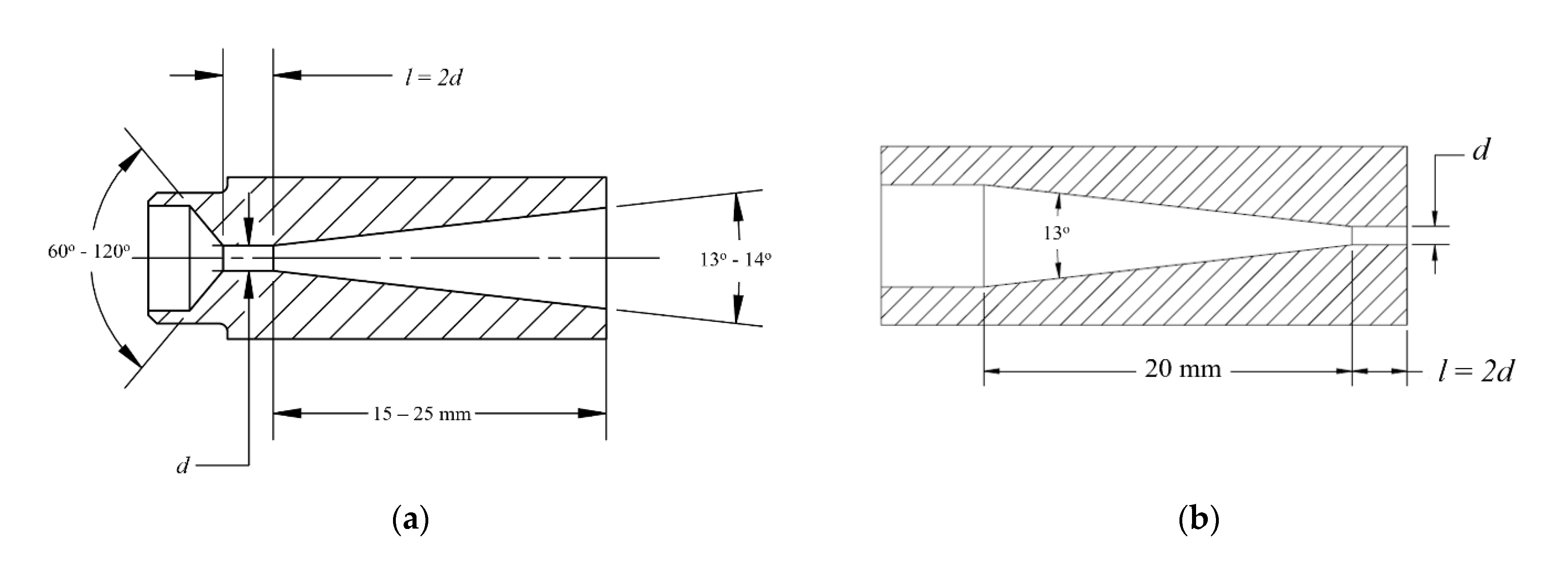
Figure 2.
Geometry of nozzle holders.

Figure 3.
Mesh structure near nozzle exit. Size of elements: 0.1 mm, 0.2 mm, 0.5 mm.
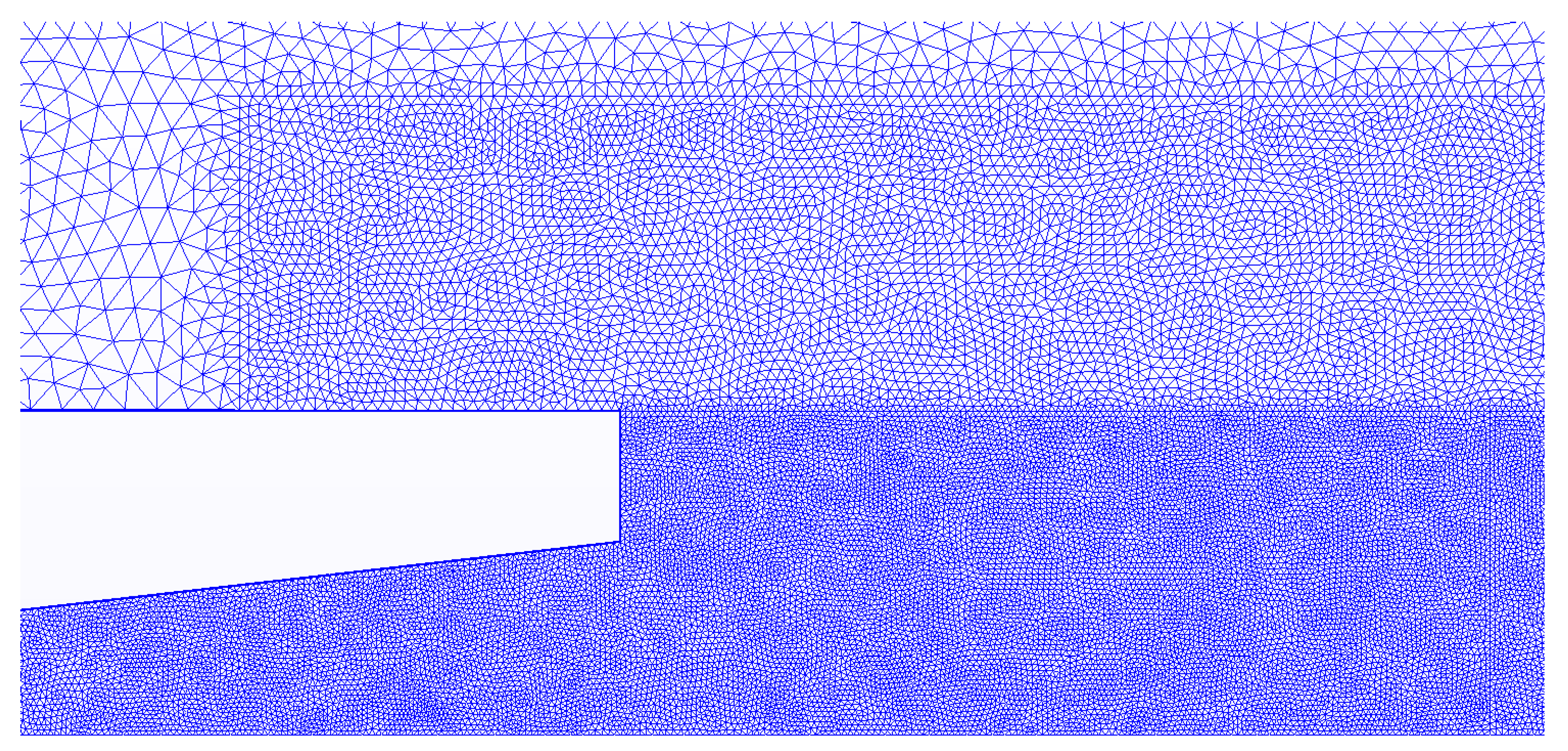
Figure 4.
Mesh study. Average cavitation vapor volume fraction at the nozzle exit.
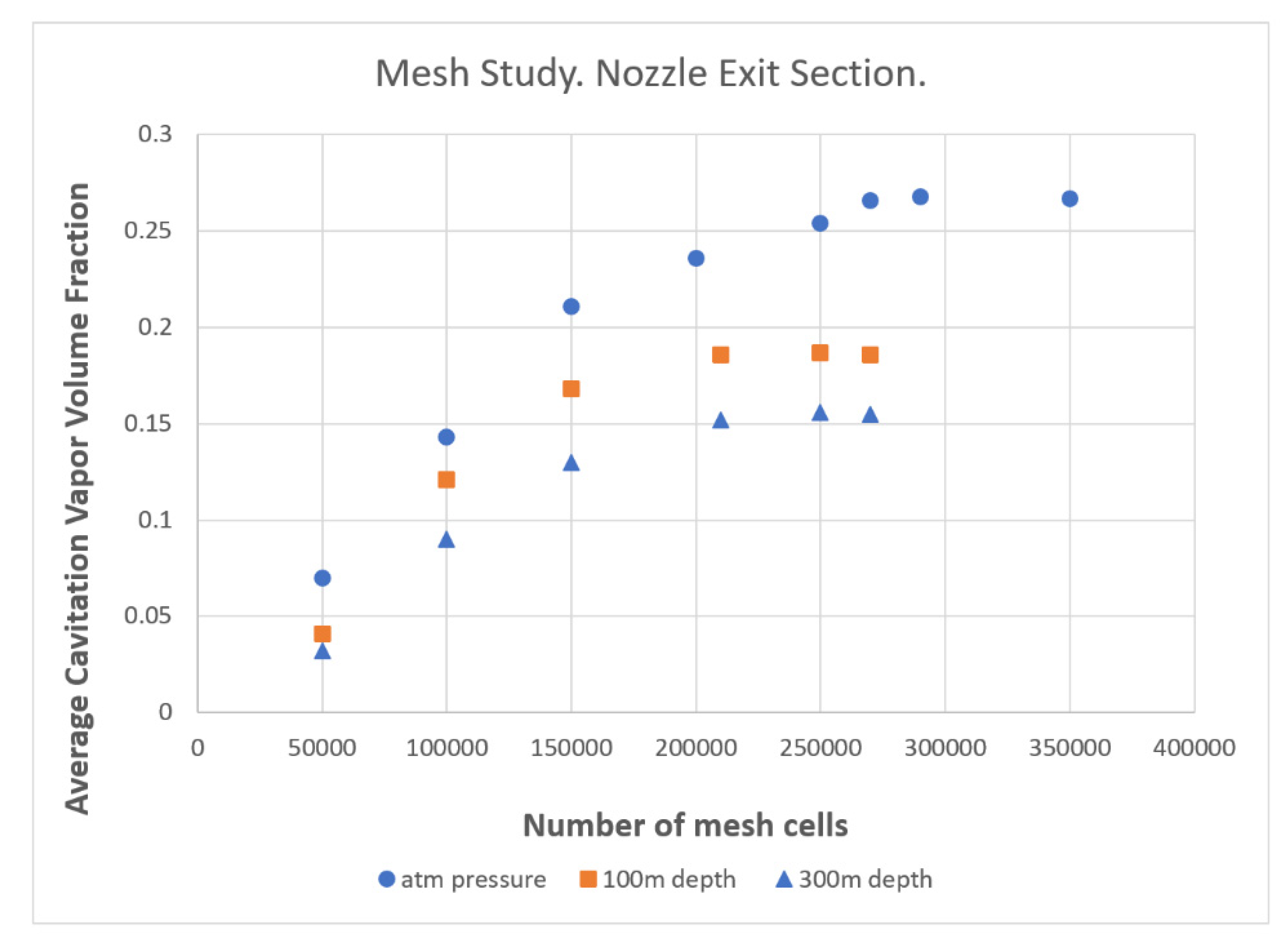
Figure 5.
Geometry and mesh structure for cavitation nozzle. Domain size: 150 cm × 20 cm.
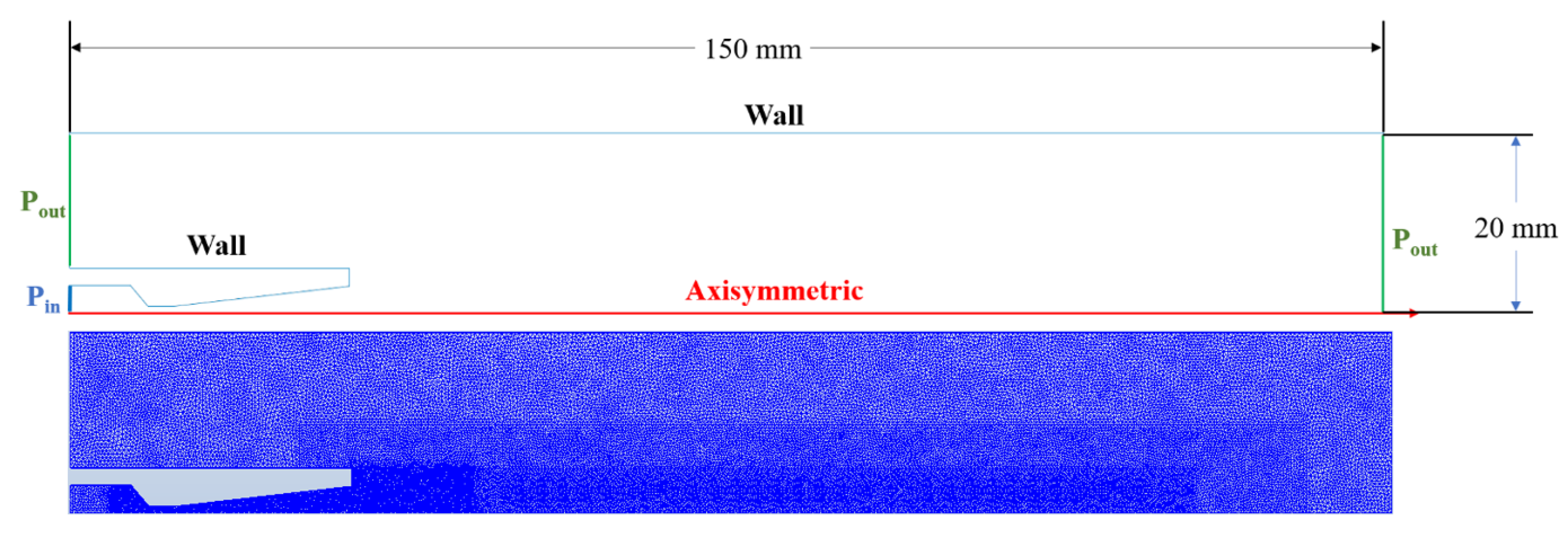
Figure 6.
Geometry and mesh structure for conical nozzle. Domain size: 150 cm × 20 cm.
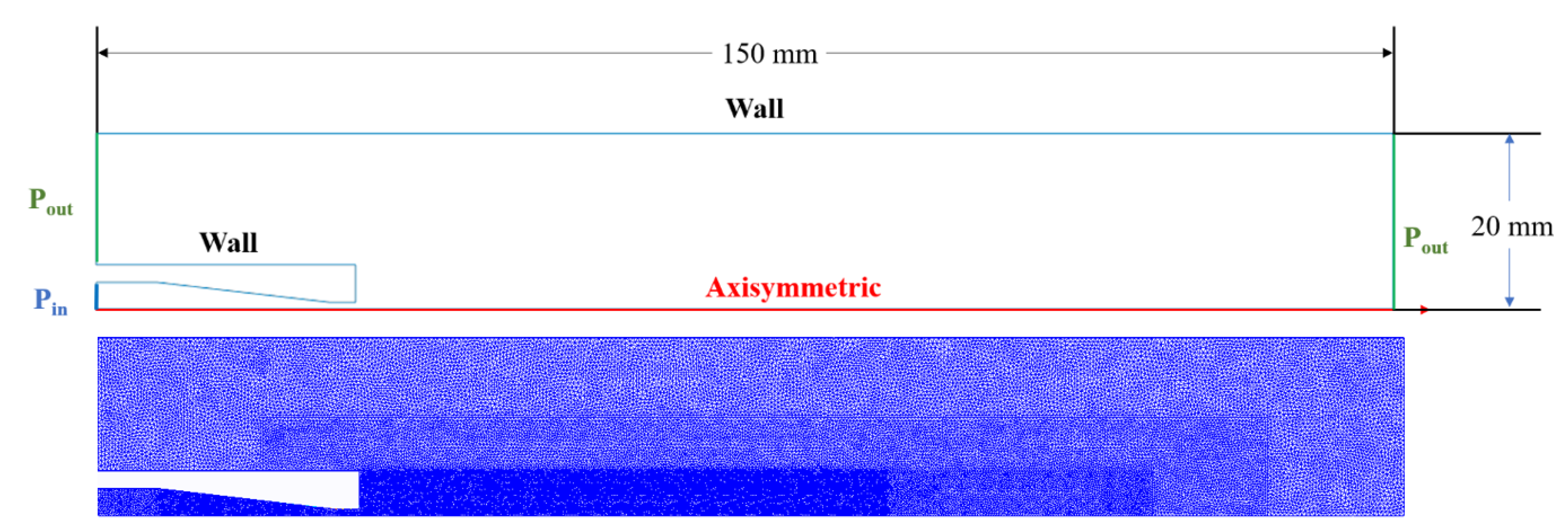
Figure 7.
Experimental setup. 1: Water tank; 2: centrifugal booster pump; 3: filter (5 μm); 4: flowmeter; 5: plunger pump; 6: high-pressure hose; 7,17: safety valves; 8,20: needle valves; 9,15: Bourdon tube pressure gauges; 10: test chamber; 11,12: lids; 13: sight glass: 14: nozzle; 16: microphone; 18: test plate; 19: holder; 21: return line.
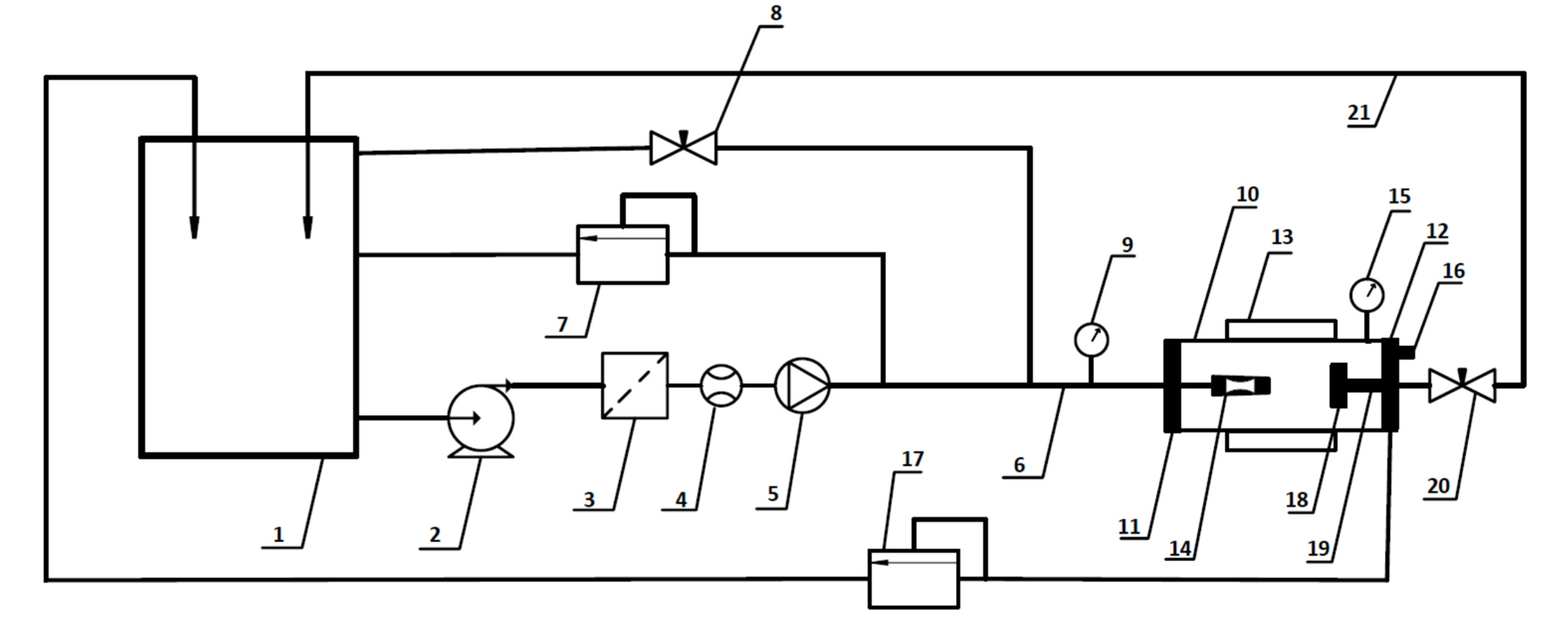
Figure 8.
Cavitation vapor volume fraction for cavitation nozzle. Pin = 300 atm: (a) Pout = 0 (gauge), (b) Pout = 10 atm (gauge), (c) Pout = 30 atm (gauge).
Figure 8.
Cavitation vapor volume fraction for cavitation nozzle. Pin = 300 atm: (a) Pout = 0 (gauge), (b) Pout = 10 atm (gauge), (c) Pout = 30 atm (gauge).
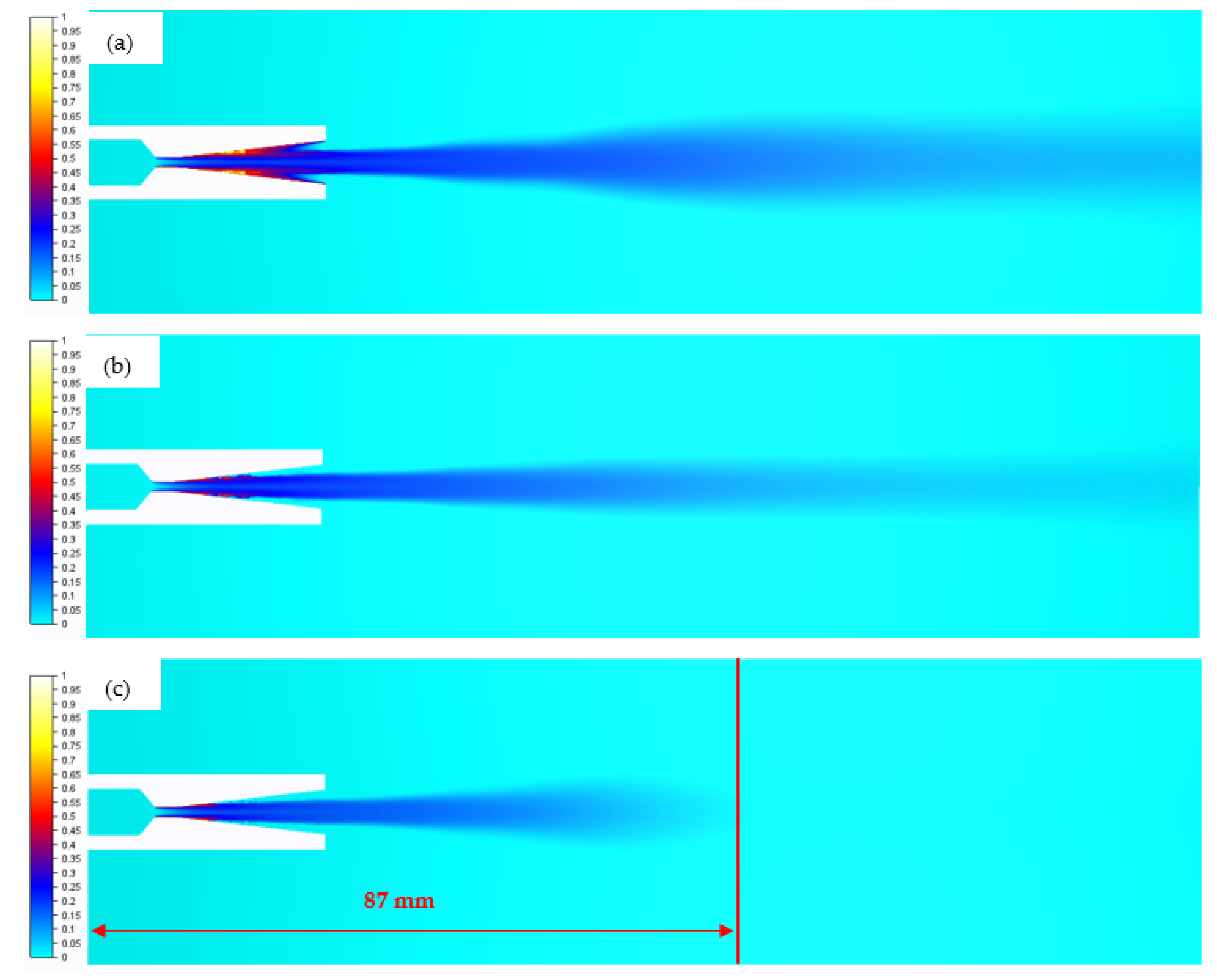
Figure 9.
Velocity (m/s), Pout = 30 atm, Pin = 300 atm. (a) Hydrodynamic nozzle, (b) cavitation nozzle.
Figure 9.
Velocity (m/s), Pout = 30 atm, Pin = 300 atm. (a) Hydrodynamic nozzle, (b) cavitation nozzle.

Figure 10.
Erosion pattern on aluminum plates. (a) Pressure in the test chamber is atmospheric, (b) pressure in the test chamber is 10 atm, (c) pressure in the test chamber is 30 atm.
Figure 10.
Erosion pattern on aluminum plates. (a) Pressure in the test chamber is atmospheric, (b) pressure in the test chamber is 10 atm, (c) pressure in the test chamber is 30 atm.
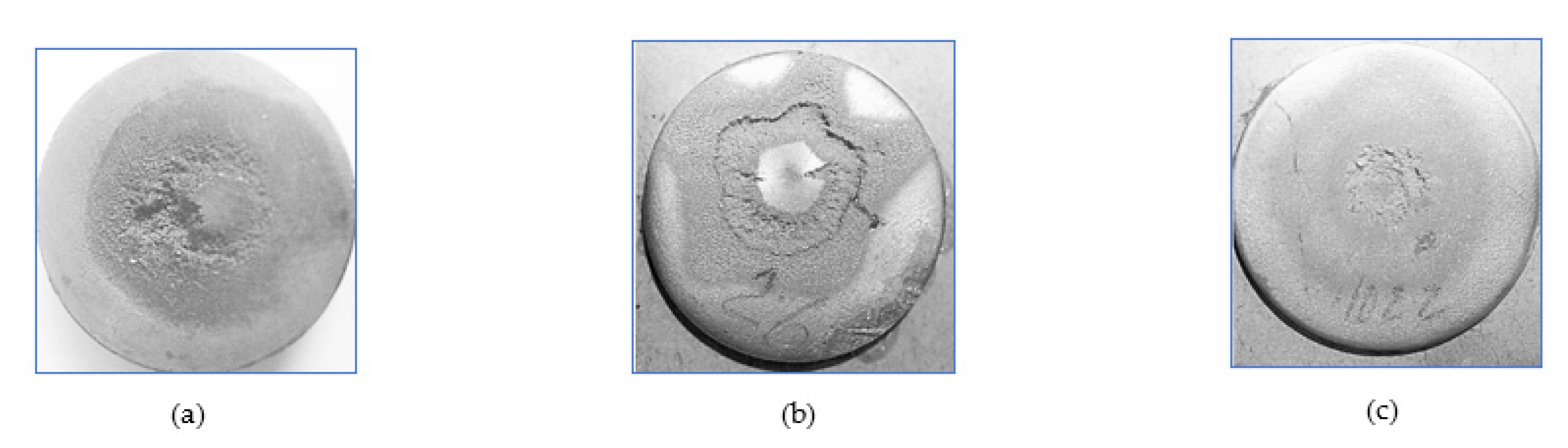
Figure 11.
Cavitating jet inside the test chamber. Pin = 300 atm: (a) Pout = 0 (gauge), (b) Pout = 10 atm (gauge), (c) Pout = 30 atm (gauge).
Figure 11.
Cavitating jet inside the test chamber. Pin = 300 atm: (a) Pout = 0 (gauge), (b) Pout = 10 atm (gauge), (c) Pout = 30 atm (gauge).

Figure 12.
Cavitation vapor volume fraction for cavitation nozzle. Pin = 300 atm: (a) Pout = 0 (gauge), (b) Pout = 10 atm (gauge), (c) Pout = 30 atm (gauge).
Figure 12.
Cavitation vapor volume fraction for cavitation nozzle. Pin = 300 atm: (a) Pout = 0 (gauge), (b) Pout = 10 atm (gauge), (c) Pout = 30 atm (gauge).
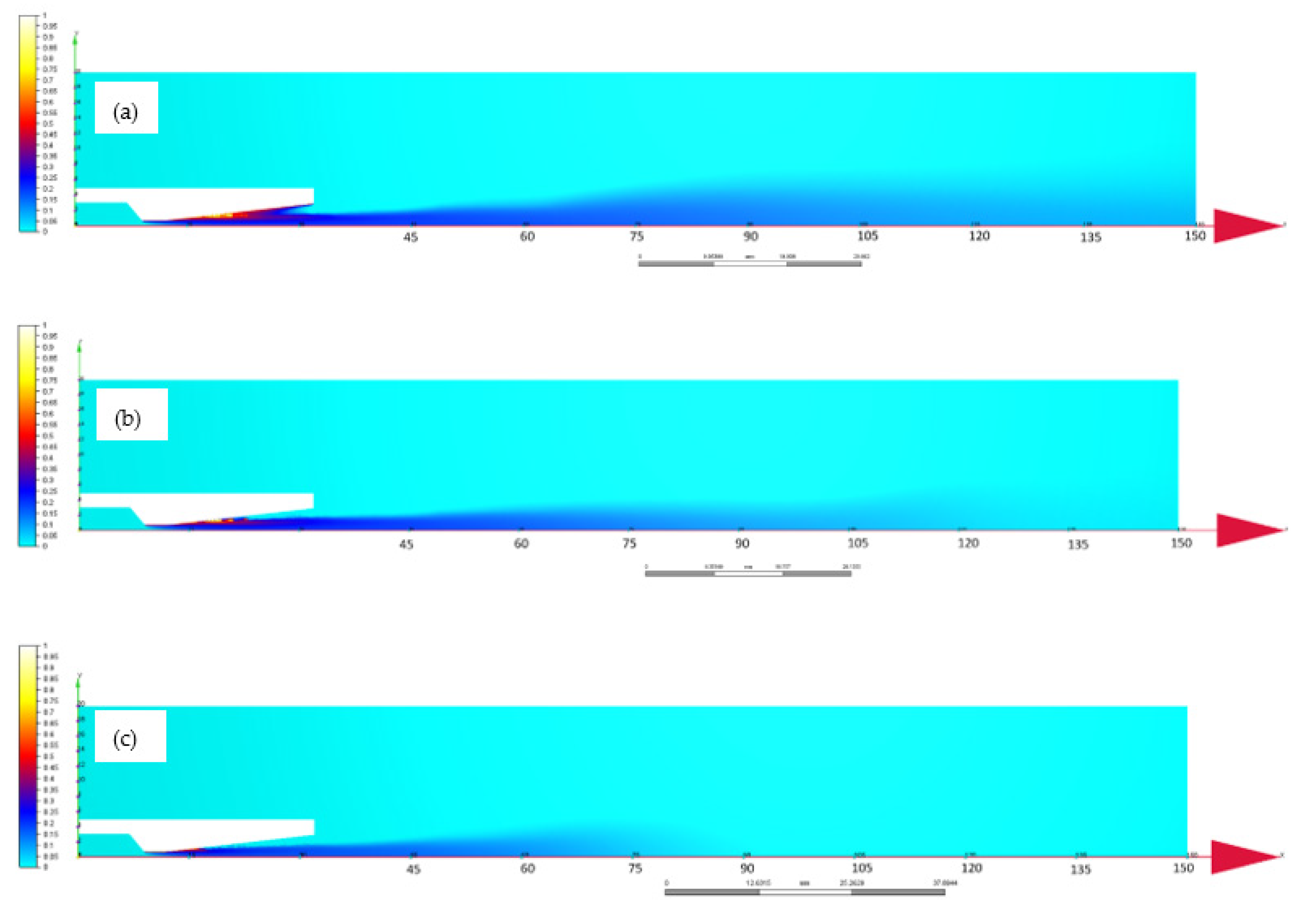
Figure 13.
Sets of nozzles ready for well cleaning. (a) Cavitation nozzles, (b) hydrodynamic conic nozzles.
Figure 13.
Sets of nozzles ready for well cleaning. (a) Cavitation nozzles, (b) hydrodynamic conic nozzles.
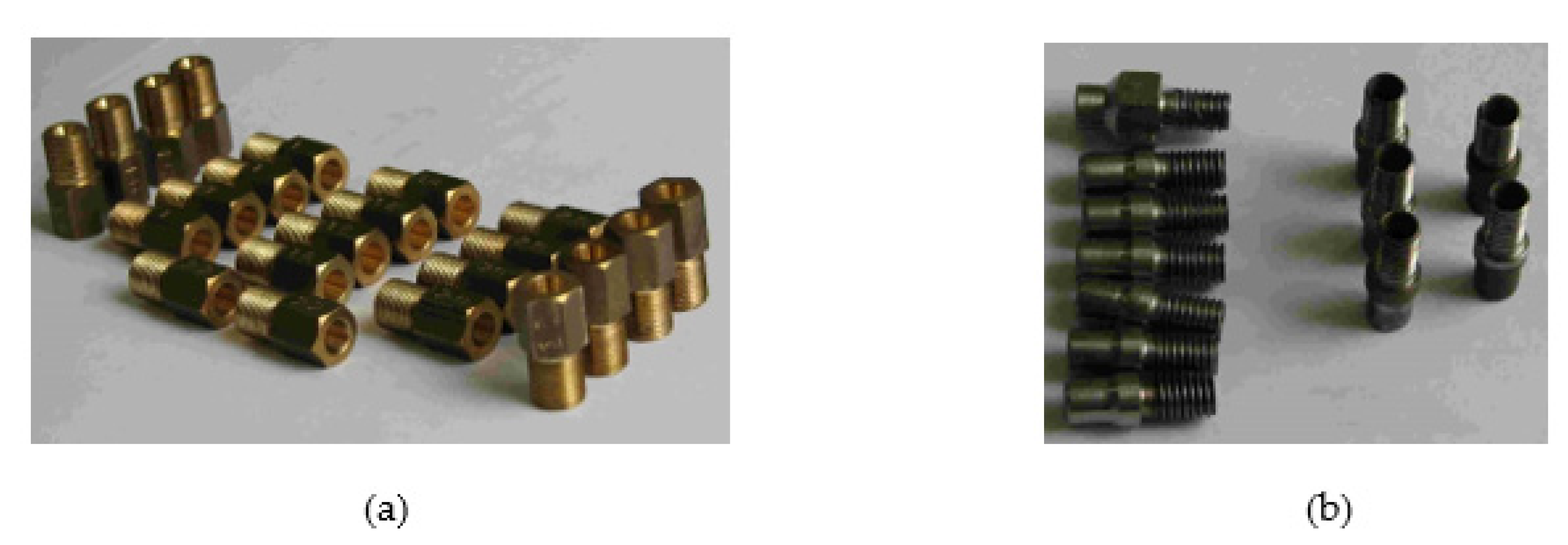
Figure 14.
Well rehabilitation operations: (a) cleaning setup, (b) mixture pumped out of the well during the cleaning, (c) submerged nozzle holder on high-pressure hose.
Figure 14.
Well rehabilitation operations: (a) cleaning setup, (b) mixture pumped out of the well during the cleaning, (c) submerged nozzle holder on high-pressure hose.


Table 1.
RNG model constants used in the model.
| Constant | Value | Result of Increasing Value |
|---|---|---|
| Cμ | 0.09 | more mixing, mores shear, greater change in pressure |
| C0 | 1.44 | less mixing, lower shear, smaller change in pressure |
| C2 | 1.92 | more mixing, more shear, greater change in pressure |
| β | 0.015 | more mixing, more shear, greater change in pressure |
| η0 | 4.38 | more mixing, more shear, greater change in pressure |
| σK | 0.7179 | (not available for user modification) |
| σε | 0.7179 | (not available for user modification) |
Table 2.
Cleaning results.
| No. of Water Well, Year of Drilling. All Wells are Located in Krasnodar Krai, Russia | Depth (m) | Flow Rate Before/After Cleaning, m3/h | Flow Rate Increase, (m3/h)/(%) | |
|---|---|---|---|---|
| Before | After | |||
| 14 (6940) 1989 (year of drilling) | 339.5 | 50 | 67 | 17/34% |
| 16 (7302) 1989 (year of drilling) | 331 | 55 | 85 | 30/54% |
| 211 2007 (year of drilling) | 306 | 6.9 | 10.2. After 2 months went up to 13 m3/h | 3.3/47.8% |
| 1 2002 (year of drilling) | 109 | 2.4 | 5.3 | 2.9/121% |
Publisher’s Note: MDPI stays neutral with regard to jurisdictional claims in published maps and institutional affiliations. |
© 2021 by the authors. Licensee MDPI, Basel, Switzerland. This article is an open access article distributed under the terms and conditions of the Creative Commons Attribution (CC BY) license (https://creativecommons.org/licenses/by/4.0/).
Share and Cite
MDPI and ACS Style
Omelyanyuk, M.; Pakhlyan, I.; Bukharin, N.; El Hassan, M. Reduction of Energy Consumption for Water Wells Rehabilitation. Technology Optimization. Fluids 2021, 6, 444. https://doi.org/10.3390/fluids6120444
AMA Style
Omelyanyuk M, Pakhlyan I, Bukharin N, El Hassan M. Reduction of Energy Consumption for Water Wells Rehabilitation. Technology Optimization. Fluids. 2021; 6(12):444. https://doi.org/10.3390/fluids6120444
Chicago/Turabian StyleOmelyanyuk, Maxim, Irina Pakhlyan, Nikolay Bukharin, and Mouhammad El Hassan. 2021. "Reduction of Energy Consumption for Water Wells Rehabilitation. Technology Optimization" Fluids 6, no. 12: 444. https://doi.org/10.3390/fluids6120444