
Thrust Vectoring of a Fixed Axisymmetric Supersonic Nozzle Using the Shock-Vector Control Method


Department of Mechanical and Aerospace Engineering, Politecnico di Torino, Corso Duca degli Abruzzi 24, 10129 Torino, Italy
*
Author to whom correspondence should be addressed.
Fluids 2021, 6(12), 441; https://doi.org/10.3390/fluids6120441
Submission received: 8 November 2021
/
Revised: 28 November 2021
/
Accepted: 2 December 2021
/
Published: 7 December 2021
(This article belongs to the Special Issue High Speed Flows)
Abstract
:The application of the Shock Vector Control (SVC) approach to an axysimmetric supersonic nozzle is studied numerically. SVC is a Fluidic Thrust Vectoring (FTV) strategy that is applied to fixed nozzles in order to realize jet-vectoring effects normally obtained by deflecting movable nozzles. In the SVC method, a secondary air flow injection close to the nozzle exit generates an asymmetry in the wall pressure distribution and side-loads on the nozzle, which are also lateral components of the thrust vector. SVC forcing of the axisymmetric nozzle generates fully three-dimensional flows with very complex structures that interact with the external flow. In the present work, the experimental data on a nozzle designed and tested for a supersonic cruise aircraft are used for validating the numerical tool at different flight Mach numbers and nozzle pressure ratios. Then, an optimal position for the slot is sought and the fully 3D flow at flight Mach number is investigated numerically for different values of the SVC forcing.
1. Introduction
Thrust Vectoring (TV) consists of the modulation of the thrust vector in a variable direction other than the axial direction, thus introducing an additional control variable in the equation of motion of the aircraft. In so doing, otherwise inoperable flight regimes, such as maneuvers at low airspeeds and very high angles of attack, or even stalled conditions, can be handled safely [1,2,3]. Moreover, designers can explore new supersonic/hypersonic aircraft configurations with lower sonic-boom signatures [4], and with Short Take-Off and Landing (STOL) capabilities and augmented maneuverability [1]. Nowadays, thrust vectoring control is a required feature for any advanced tactical fighter [3,5]. Practical application of thrust vectoring is obtained by turning the nozzle mechanically to point in different directions. The same effect can be obtained without actuated mechanical hardware, by forcing and manipulating the flow inside a nozzle of fixed geometry. This second approach, namely the Fluidic Thrust Vectoring (FTV), uses a secondary air bleed in order to actively manipulate and control the primary air-stream of the nozzle. The injected fluid creates variable “artificial” nozzle boundaries and the perturbations generated by the forcing of the secondary flow make the nozzle wall pressure distribution asymmetric. The resulting effect is a side-force on the nozzle that can be seen as the lateral component of the thrust vector. Experimental testing and numerical simulations of simple two-dimensional nozzle configurations have shown significant thrust deflections and a dynamic response faster than that obtained by mechanical systems [6,7,8]. Moreover, with respect to mechanical thrust vectoring, the FTV approach does not increase the aircraft weight significantly.
Following the renewed interest in space exploration and the trans-atmospheric supersonic flight, FTV concepts are being intensively investigated [9,10,11,12,13]. The key point for the fluidic approach is the identification of manipulation techniques that gradually modulate the nozzle wall pressure symmetry-breaking effect within an acceptable range of deterioration of the nozzle performances [14]. Several control strategies have been investigated in the literature including techniques such as Shock Vector Control (SVC), Counter-Flows (CF), Throat Shifting (TS) and supersonic Dual-Throat Nozzle (DTN) [14]. The effectiveness of the mentioned FTV techniques has been investigated numerically and tested experimentally by several research groups [4,7,15,16,17,18,19,20,21,22,23]. The integration of FTV models in engine and aircraft dynamic models is an on-going research project [24,25,26]. Most current experimental and numerical investigations on FTV rely on fundamental aspects and are based on two-dimensional nozzle models [14]. Two-dimensional flows are easier to visualize experimentally and less expensive from a computational point of view, while retaining most of the essential features of the phenomenon under investigation. More commonly, however, aircraft and rocket nozzles are axisymmetric and this fact has an important consequence: after breaking the flow symmetry, for example, by local secondary air-injection, the nozzle flow becomes fully three-dimensional. Therefore, the applications of FTV to real nozzle geometries must deal with the analysis and/or simulation of fully three-dimensional flows.
In the present work, the FTV performances of an axisymmetric nozzle under shock vector control are investigated numerically. In order to support our analysis with experimental data, the reference nozzle geometry is deduced from the experimental work of Carlson and Lee at Nasa LaRC [27]. Five different nozzle geometries were tested in that reference. Each nozzle geometry represented a different flight condition and power setting of a variable-geometry axisymmetric nozzle designed for a variable-cycle engine of a supersonic aircraft. The nozzle was installed in a nacelle with a forebody and was tested at external flow Mach numbers ranging from 0.6 to 1.3 [27]. The nozzle configuration 2 at Mach flight number , and was selected for the present analysis. The outline of the papers is as follows: the nozzle setup and working conditions are described first; then the mathematical model and numerical approaches are illustrated. After that, the numerical investigations follow with increasing complexity. The numerical tools are validated with respect to experimental data [27] in the axisymmetric case for different values of the Nozzle Pressure Ratio npr and different Flight Mach numbers. As a second step, the sensitivity of the flow to the slot position and secondary mass flow is investigated, retaining the axisymmetric assumption. The SVC approach is then finally applied to the fully three-dimensional case and the nozzle FTV effectiveness and performances are investigated numerically for different values of the secondary mass flow.
2. Nozzle Setup and Geometry
The nozzle geometry and working conditions simulated in the present numerical study are derived from the experimental testing carried out at Nasa LaRC by Carlson and Lee [27]. In that work, five models of an axisymmetric, convergent-divergent nozzle with circular-arc throat contour and conical divergent sections were investigated experimentally. The nozzle geometries refer to different configurations of the variable-geometry axisymmetric nozzle designed for a supersonic cruise aircraft equipped with a variable-cycle engine. The five configurations represent the nozzle setup for different flight conditions and power settings ranging from a subsonic cruise, dry power configuration, characterized by a low expansion ratio and a high nozzle boattail angle, to supersonic acceleration, with maximum afterburning, having a high expansion ratio and a low nozzle boattail angle. The experimental investigations were conducted at nozzle pressure ratios (npr) from jet-off to about npr and for freestream Mach numbers ranging from 0.60 to 1.30. A detailed description of the nozzle geometries and testing conditions is given in Ref. [27]. Numerical simulations of the flow are also available for comparison [28,29]. The nozzles were attached to an axisymmetric nacelle with a forebody. The general arrangement of the nacelle model and support system is shown in Figure 1. Nozzle Configuration 2 (Conf-2) of Ref. [27] has been selected for the numerical tests reported here. The configuration corresponds to the supersonic cruise setting in dry condition, that is, without afterburning. The adaptation pressure ratio of the nozzle in Conf-2 is npr. Nozzle geometry and relevant design parameters are presented in Figure 2.
3. Mathematical and Numerical Modelling
The problem is numerically investigated solving the compressible Unsteady Reynolds-Averaged Navier–Stokes (URANS) equations by using the commercial CFD solver STAR-CCM+ [30]. The one-equation model of Spalart–Allmaras (S-A) [31,32] is used for the turbulence modelling, as it has shown a good agreement with the experimental data for the case of unsteady flow in nozzles [7,33]. The numerical approach adopted is almost equivalent to that used in the in-house 2D numerical framework developed for the unsteady simulation of the vectored nozzle in open and closed-loop conditions, which was tested and validated for the FTV with both continuous or pulsating blowing [6,34].
Briefly, the flow governing equations are represented by the compressible Unsteady Reynolds Averaged Navier–Stokes equations (URANS), written in the compact integral form:
for an arbitrary volume enclosed in a surface . With the usual conventions, is the hyper-vector of conservative variables, and are tensors containing the inviscid and the viscous fluxes, respectively.
is the velocity vector, E the total energy per unit volume, is the ratio of the specific heats and is the unit matrix. The term
contains turbulence model source terms. The viscous stresses terms can be written as:
The laminar viscosity is computed via the Sutherland’s law, whereas the turbulent viscosity is defined according to the Spalart–Allmaras (S-A) model [31,32]. Inviscid fluxes are evaluated through the AUSM+ flux–vector splitting scheme [35], based on the upwind concept, which applies to both the convective and pressure parts of the inviscid flux. The computation takes into account local flow characteristics for a correct propagation of physical information inside the domain. A second order discretization in space and time has been chosen for the solution of the set of equations, by means of an implicit, dual time-stepping solver. The implicit solver features a preconditioned pseudo-time derivative term within the equation system. This additional term vanishes as convergence is reached in the inner loop, and the solution at the next physical time level is computed. A local pseudo time-step is used in steady state simulations and for inner loop iterations of transient simulations.
Computational Domain and Boundary Conditions
The domain geometry is chosen in such a way to capture the relevant interactions between the free flowing air and the forebody, as well as interactions between the external flow and the nozzle jet. The computational domain consists of a mesh of about 170 k quadrangular elements for the 2D axisymmetric analysis, whereas for 3D calculations, a grid of about 3.5 M cells has been generated by revolution around the symmetry axis. The boundary conditions for the problem were chosen according to the nature of the flow and the available experimental information. For the external flow inlet, a free-stream boundary condition has been used to impose Mach number, pressure and temperature. A pressure outlet boundary is utilized to impose an outflow condition with specified static ambient pressure, while values for velocity or temperature are extrapolated from the interior of the domain. A total inlet condition is adopted for the nozzle flow, in order to prescribe values of total pressure and total temperature for the jet, whereas for the injection of the secondary flow, a mass flow rate boundary condition has been used. For solid surfaces a no-slip wall condition is utilized. For the 2D domain a symmetry axis has been prescribed in order to perform the axisymmetric simulations, whereas for the 3D simulation a symmetry plane condition is utilized to account for the other half of the physical domain. A representation of the computational grid and a visualization of the boundaries can be found in Figure 3.
4. Numerical Results
4.1. Grid Independence Analysis
The number of nodes for the axisymmetric mesh has been defined after a grid dependence study on three different levels of refinement. A coarse grid of 73 k cells, a medium grid of 170 k cells, and a fine grid of 325 k cells have been selected for this analysis. The results, in terms of temperature, mach number and pressure profiles obtained along the x-axis, that is, along the nozzle axis of symmetry on the different grids, are presented in Figure 4. A small mismatch can be appreciated between the temperature profile obtained on the coarse mesh with respect to that obtained on the medium and fine meshes (Figure 4a). The latter two temperature profiles match perfectly instead. The coarse grid also tends to slightly under-predict the Mach number values, as visible in Figure 4b. Nevertheless, the pressure distributions along the x-axis evaluated on the three meshes are almost indistinguishable (Figure 4c). The x-axis is also the region of inner nozzle computational domain with the lower resolution. A refinement of the mesh has been performed to increase the resolution of the results near walls and other regions of interest as, for instance, at the exit section of the nozzle and in the vicinity of the secondary flow injection opening. The grid has also been stretched near the walls in order to obtain , and in such a manner that no wall functions were needed to correctly model turbulence at the boundary layer level. Although the coarsest mesh provided more than adequate results for the wall pressure distributions, the medium grid was chosen for all subsequent analyses for its greater resolution inside the nozzle duct and the increased shock capturing accuracy.
4.2. Simulation of the Axisymmetric Nozzle Flow
The flowfield in an axisymmetric propulsive nozzle is very complex and is characterized by a highly nonlinear response to incoming perturbations. An extensive validation of the computational framework used must be carried out before going toward the simulations of fluidic forcing. As mentioned in previous sections, the wide database of experiments reported in Carlson and Lee [27] offers very useful test-cases for this kind of validation, including the effects of external flow interference at different nozzle pressure ratios. In this section, the validation carried out for nozzle configuration 2 (Conf-2) of Ref. [27], without SVC forcing, is described with details. Three different flight Mach number conditions have been selected for the validation, specifically , and , in order to obtain a fairly complete set of working conditions for the nozzle, ranging from relatively low flight Mach numbers to supersonic cruise conditions, and across a variety of nozzle pressure ratios. For validation purposes, the selected sets of parameters (, npr) match the working conditions tested in the NASA LaRC experiments [27].
A full view of the simulated flowfield inside and around the nozzle system is presented in Figure 5. This flowfield represents a typical nozzle off-design condition of interest. The nozzle is over-expanded (the pressure ratio is npr ) at high transonic flight (). As is visible, an adequate resolution of the nozzle plume is obtained and no significant flow perturbations arise from or reach the boundaries, other than the jet flow. Moreover, the interference generated by the forebody does not propagate up to the nozzle region. Therefore, the jet flow issuing from the nozzle is influenced only by the external pressure and by the flow conditions in the aft-body region in general.
The results of the complete sets of simulations at = 0.6, = 0.9 and = 1.2 are presented in Figure 6, Figure 7 and Figure 8, respectively. For each pressure ratio, the flowfield is represented in terms of both Mach number and density contour maps. The nprs values are not the same for each flight mach number in order to adhere to that reported in the experiments [27]. In all these figures, the different levels of nozzle over-expansion, its effect of the shock induced separation and on the mach disk position is clearly visible. Focusing on Figure 6, once the nozzle flow becomes supersonic, shock structures begin to form, as is already visible for npr , where oblique shock waves and the Mach disk are first generated. As the npr is increased, the region of separated flow shrinks in size, the Mach disk is shifted forward, and wave reflections become more visible. For even higher npr, supersonic shocks and reflections become increasingly distinguishable in the jet plume too. The density field follows the same considerations, but its values mirror those of the Mach field, decreasing during expansions where the Mach number increases and vice versa through shocks. Very similar results are obtained for external Mach numbers and , as illustrated in Figure 7 and Figure 8.
The plots of numerical results against available experimental data are given in Figure 9, for both the pressure coefficient on the boat-tail , and pressure distribution on the internal wall, normalized with the jet total pressure . A good agreement between numerical and experimental data is achieved with the chosen model, as the point of separation was accurately predicted in all cases. The best results are obtained at higher nozzle pressure ratios, in particular for npr , where the separated regions are at first limited and then eliminated. The external pressure coefficient plots also show good agreement with experimental values, following the curve compression and expansion features for all three flight Mach numbers. The higher mismatch between numerical and experimental data is obtained at and npr in Figure 9c. At that conditions, the numerical prevision shows a choked flow inside the nozzle, whereas the experimental data do not collapse in a single curve after chocking as expected and the flow seems to exhibit a weak separation instead of an abrupt shock induced separation. After that, the location of the flow separation and the exit conditions are matched correctly.
4.3. Application of Secondary Injection to the Axisymmetric Nozzle Flow
In this section, a study of the flow forcing effectiveness is carried out for identifying an adequate location of the secondary massflow injection point required for the SVC based thrust vectoring. Obviously, under the axisymmetric flow assumption, we do not expect any jet flow deflection. It was assumed, anyway, that the flow forcing may produce local effects that are similar in the axisymmetric and fully three-dimensional case. It is well-known that the SVC technique depends on a flow structure generated by the interaction between the secondary blowing, normal to the wall, and the main flow. In the supersonic region upwind the flow injection a fluid ramp is formed and an oblique shock is generated [20,36]. We are interested in the numerical estimation of parameters such as the shock distance from the injection slot and the shock inclination, in order to rapidly assess the effects on the main flow and to identify a suitable position of the injection slot for the more costly 3D simulations. Naturally, multiple parameters other than the position of the slot alone can influence the effect of the injection on the main flow and its structures; for instance, the secondary mass flow ratio and the opening area have been shown to have a direct influence on the deflection of the flow [37]. In this preliminary analysis, the secondary mass flow-rate has been kept constant and equal to 3% of the main mass flow-rate, while the injection slot area in the axisymmetric case is naturally the lateral surface of a truncated cone. The resulting mass flux per unit area is thus considerably smaller than that in the case of a secondary injection of the same mass flow-rate through a reduced area. The opening has been sequentially positioned at 70%, 80% and 90% of the length of the diverging part of the nozzle until the position of the fluidic ramp that would be generated was considered satisfactory for the subsequent fully three-dimensional analysis. The modification of the grid close to the injection slot and the required grid refinement are shown in Figure 10.
As can be seen in Figure 11, the recession of the injection slot position moves the first oblique shock backwards, and expands the separated flow region near the slot. When the opening position is too far upstream a reattachment of the flow can be seen for this value of the mass flux per unit area, however this problem is eliminated when either the injection area is restricted or the mass flux per unit area is increased, or both. A comparison between the perturbation of the main flow in axisymmetric conditions and in three dimensions, for the same position of the slot and the same value of mass flux is shown in Figure 12. The chosen mass flux for the comparison is that corresponding to a secondary injection of 6% of total mass flow rate in the three dimensional case. The increase in value of the mass flux eliminates the aforementioned problem of reattachment of the flow for the axisymmetric case and, as can be seen in the figure, the effect of the injection in these conditions is more pronounced than that in the three dimensional case. With these considerations in mind, the slot position at 70% of the nozzle length has been considered the most adequate for the purposes of the subsequent three dimensional analysis.
4.4. SVC Thrust Vectoring of the Axisymmetric Nozzle in 3D
In this section, the analysis based on the fully three-dimensional numerical simulations of the nozzle under SVC forcing is discussed. In previous SVC vectored nozzle studies [19,20,36,38] performances are analyzed and characterized by varying the npr and the secondary mass flow ratio smf for a jet-flow efflux in calm air. External flow interactions have been accounted for mainly by CFD approaches in two dimensions [39]. In Section 4.2, the NASA test-case on boat-tail nozzle flow has been used for validating the numerical tools and a good agreement for the simulations of the interaction between the nozzle plume and the external flow has been obtained for the case of co-flowing streams at different asymptotic Mach numbers . Now, we follow the same path and numerically analyze the SVC effects of secondary mass flow injection on the nozzle side force, also in the presence of an external flow. In particular, at this stage, we focused on the study of the effectiveness of the FTV for different levels of forcing, based on different smf values, at the nozzle pressure ratio npr and with an external flow Mach number .
The 3D grid has been generated by rotational extruding of the axisymmetric mesh by an angle of 180° around the symmetry axis while retaining symmetry on the meridian plane. Only the half nozzle has therefore been simulated because of symmetry. A 3D grid of about 3.5 M cells is thus obtained. A sketch of the nozzle configuration is shown in Figure 13. Based on the analysis described in the previous section, the injection slot, with a 2 mm width in the axial direction, has been positioned at 70% of the axial extension of the diverging part of the nozzle. The slot has been extended by a degree angle along the circumferential coordinate. Due to the symmetry assumption, the actual circumferential extension of the slot is twice, that is = 90°. Figure 13 also shows the injection slot and its location on the nozzle walls.
Various secondary mass flow rates smf have been considered, ranging from 3% to 10% of the main flow rate computed through the nozzle throat. The FTV performances have been evaluated as is done in [11]. In particular, the thrust components along the axes have been computed and the ratio of lateral force component to the axial component gives a measure of the vectoring effectiveness of the secondary flow injection. Results obtained by the numerical simulations are reported in Figure 14 where the values of the pitch thrust-vector angle at different smf are shown.
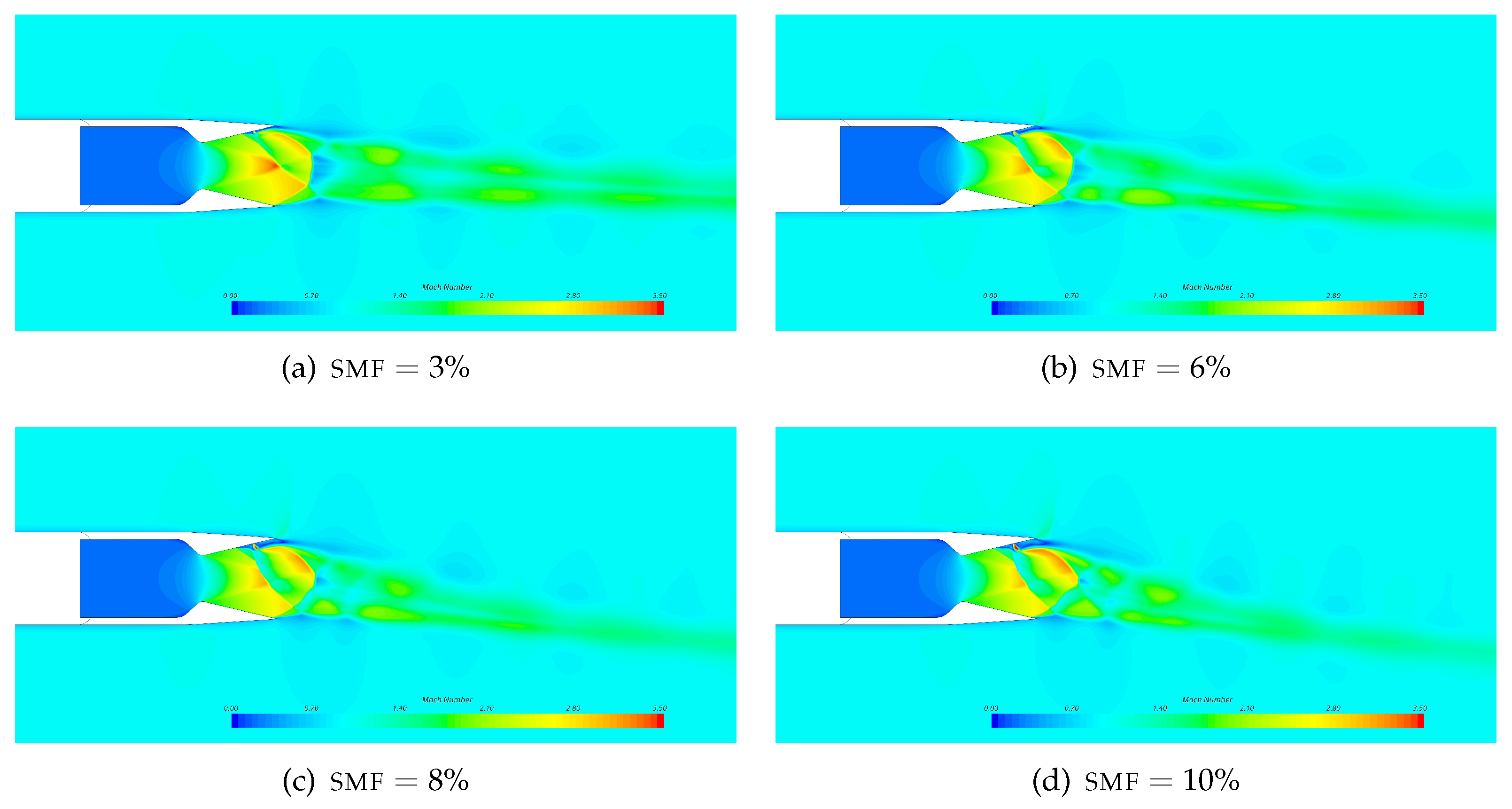
The plot of Figure 14 shows that the increase of secondary mass flow rate induces a nonlinear increase in the value of , up to about for smf , following an almost parabolic curve [11]. As a consequence, the lateral force rises as well, increasing from 3.5% to about 7.5% of the axial force component, . At the same time, the axial force component is reduced with respect to the symmetric condition of just about 3%, passing from about 1280 N for smf to 1245 N for smf = 10%. The increase in lateral force is due to the separation induced by the injection of the secondary flow, which in turn generates a separation zone on the nozzle walls, thus changing the pressure distribution as is well highlighted in Figure 15 for the 6% and 10 % of secondary mass flow cases. Such separation is shown in Figure 16, where it is very clear that a fluidic ramp is formed ahead of the injection point, generating an oblique shock that induces the flow to separate, changing the pressure distribution and generating a force imbalance, (). Naturally, the separation zone increases as the smf rises; however, this phenomenon does not seem to overly affect the axial force (). This last consideration gives us expectation that the method can be applied efficiently to vector the thrust of propulsion systems.
5. Conclusions
Numerical investigations of the active flow control of an axisymmetric nozzle by using SVC at flight mach number have been carried out. With respect to the large part of the works available in the open literature, the present study involves an axisymmetric nozzle geometry, which makes the jet-flow fully three-dimensional, and the presence of a non-negligible effect of the external flow. While fluidic thrust vectoring experiments and simulations of axisymmetric nozzles discharging in calm air are readily available in the literature (even from the present research group [12]); to the authors’ knowledge there are no similar experiments including external flow interactions.
The present study has therefore been conceived as a design of experiment by applying the SVC thrust vectoring approach to an actual nozzle geometry, tested experimentally at NASA LaRC for non-vectored performances at several flight Mach numbers [27]. The analysis of the 3D flow was the last part of the following three-step process: (i) validation of the numerical framework against the NASA LaRC experimental data set [27]; (ii) numerical investigation of the nozzle sensitivity to SVC flow forcing; (iii) fully 3D verification of the SVC vectoring approach applied to the aforementioned nozzle.
The availability of experimental data on the external–internal flow interaction allowed for the validation of the numerical code against more realistic nozzle flow patterns, as opposed to just the efflux in calm air. The computations of the non-vectored performances in the axisymmetric case have been validated for several nozzle pressure ratios npr and at flight Mach numbers and . The numerical results and experimental data were in good agreement. The computed flowfields illustrated with detail the flow topology resulting from the interactions between the internal and external flows, and the differences between subsonic and supersonic external air-streams. Before going towards three-dimensional simulations, the sensitivity of the nozzle system to SVC forcing for different locations of the injection point has been investigated in the axisymmetric case. In fact, we assumed that local effects of fluid forcing are similar in the axisymmetric and fully three-dimensional case, and that this might provide useful insight for a suitable placement of the injection slot. Finally, the effectiveness of the SVC forcing of the nozzle in three-dimensions has been investigated numerically for different secondary mass flows at the intermediate flight Mach number and at the npr . The results show a significant turning of the thrust-vector caused by the force imbalance in the y-direction, with very limited losses of axial force .
Author Contributions
Conceptualization, E.R., R.M. and M.F.; methodology, E.R., R.M. and M.F.; software, E.R., R.M. and M.F.; validation, E.R., R.M. and M.F.; formal analysis, E.R., R.M. and M.F.; investigation, E.R., R.M. and M.F.; resources, E.R., R.M. and M.F.; data curation, E.R., R.M. and M.F.; writing—original draft preparation, E.R., R.M. and M.F.; writing—review and editing, E.R., R.M. and M.F.; visualization, E.R., R.M. and M.F. All authors have read and agreed to the published version of the manuscript.
Funding
This research received no external funding.
Institutional Review Board Statement
Not applicable.
Informed Consent Statement
Not applicable.
Data Availability Statement
Not applicable.
Acknowledgments
Computational resources were provided by [email protected], a project of Academic Computing within the Department of Control and Computer Engineering at Politecnico di Torino (http://www.hpc.polito.it).
Conflicts of Interest
The authors declare no conflict of interest.
Nomenclature
| pressure coefficient on the boat-tail, | |
| nozzle axial force | |
| nozzle normal force | |
| length of nozzle divergent part, | |
| external flow Mach number, flight Mach number | |
| external flow static pressure | |
| primary flow total pressure | |
| external flow velocity | |
| primary mass flow rate | |
| secondary mass flow rate | |
| position of the injection slot | |
| position of nozzle throat | |
| position of nozzle trailing edge | |
| pitch thrust-vector angle, | |
| external flow density | |
| npr | nozzle pressure ratio, |
| smf | secondary mass flow rate, |
References
- Asbury, S.; Capone, F. High-Alpha Vectoring Characteristics of the F-18/HARV. J. Propuls. Power 1994, 10, 116–121. [Google Scholar] [CrossRef]
- Wilde, P.; Crowther, W.; Buonanno, A.; Savvaris, A. Aircraft Control Using Fluidic Maneuver Effectors. In Proceedings of the 26th AIAA Applied Aerodynamics Conference, Honolulu, Hawaii, 18–21 August 2008. [Google Scholar] [CrossRef]
- Mason, M.; Crowther, W. Fludic Thrust Vectoring for Low Observable Air Vehicles. In Proceedings of the 2nd AIAA Flow Control Conference, Portland, OR, USA, 28 June–1 July 2004. [Google Scholar] [CrossRef]
- Flamm, J.; Deere, K.; Mason, M.; Berrier, B.; Johnson, S. Design enhancements of the Two-Dimensional, Dual Throat Fluidic Thrust Vectoring Nozzle Concept. In Proceedings of the 3rd AIAA Flow Control Conference, San Francisco, CA, USA, 5–8 June 2006. [Google Scholar] [CrossRef] [Green Version]
- Orme, J.; Sims, R. Selected Performance Measurements of the F-15 ACTIVE Axisymmetric Thrust-Vectoring Nozzle. In Proceedings of the 4th ISABE Symposium, Florence, Italy, 5–10 September 1999. [Google Scholar]
- Ferlauto, M.; Marsilio, R. Open and Closed-Loop Responses of a Dual-Throat Nozzle during Thrust Vectoring. In Proceedings of the 52nd AIAA/SAE/ASEE Joint Propulsion Conference, Salt Lake City, UT, USA, 25–27 July 2016. [Google Scholar] [CrossRef]
- Ferlauto, M.; Marsilio, R. Numerical Investigation of the Dynamic Characteristics of a Dual-Throat Nozzle for Fluidic Thrust-Vectoring. AIAA J. 2017, 55, 86–98. [Google Scholar] [CrossRef]
- Gu, R.; Xu, J. Dynamic experimental investigations of a bypass dual throat nozzle. ASME J. Eng. Gas Turbines Power 2015, 137, 084501. [Google Scholar] [CrossRef]
- Warsop, C.; Crowther, W.J. Fluidic Flow Control Effectors for Flight Control. AIAA J. 2018, 56, 3808–3824. [Google Scholar] [CrossRef]
- Warsop, C.; Crowther, W.; Forster, M. NATO AVT-239 Task Group: Supercritical Coanda based Circulation Control and Fluidic Thrust Vectoring. In Proceedings of the AIAA Scitech 2019 Forum, San Diego, CA, USA, 7–11 January 2019. [Google Scholar] [CrossRef]
- Ferlauto, M.; Ferrero, A.; Marsicovetere, M.; Marsilio, R. Differential Throttling and Fluidic Thrust Vectoring in a Linear Aerospike. Int. J. Turbomach. Propuls. Power 2021, 6, 8. [Google Scholar] [CrossRef]
- Marsilio, R.; Ferlauto, M.; Hadi Hamedi-Estakhrsar, M. Numerical simulation of a vectored axisymmetric nozzle. AIP Conf. Proc. 2020, 2293, 200018. [Google Scholar] [CrossRef]
- Takahashi, H.; Munakata, T.; Sato, S. Thrust Augmentation by Airframe-Integrated Linear-Spike Nozzle Concept for High-Speed Aircraft. Aerospace 2018, 5, 19. [Google Scholar] [CrossRef] [Green Version]
- Deere, K. Summary of Fluidic Thrust Vectoring Research Conducted at NASA Langley Research Center. In Proceedings of the 21st AIAA Applied Aerodynamics Conference, Orlando, FL, USA, 23–26 June 2003. [Google Scholar] [CrossRef]
- Deere, K.; Flamm, J.; Berrier, B.; Johnson, S. Computational Study of an Axisymmetric Dual Throat Fluidic Thrust Vectoring Nozzle for a Supersonic Aircraft Application. In Proceedings of the 43rd AIAA/ASME/SAE/ASEE Joint Propulsion Conference & Exhibit, Cincinnati, OH, USA, 8–11 July 2007. [Google Scholar] [CrossRef] [Green Version]
- Deng, R.; Kim, H. A study on the thrust vector control using a bypass flow passage. Proc. IMechE Part G J. Aerosp. Eng. 2015, 5, 1722–1729. [Google Scholar] [CrossRef]
- Deng, R.; Setoguchi, T.; Dong Kim, H. Large eddy simulation of shock vector control using bypass flow passage. Int. J. Heat Fluid Flow 2016, 62, 474–481. [Google Scholar] [CrossRef]
- Gu, R.; Xu, J.; Guo, S. Experimental and Numerical Investigations of a Bypass Dual Throat Nozzle. ASME J. Eng. Gas Turbines Power 2014, 136, 084501. [Google Scholar] [CrossRef]
- Chouicha, R.; Sellam, M.; Bergheul, S. Effect of reacting gas on the fluidic thrust vectoring of an axisymmetric nozzle. Propuls. Power Res. 2020. [Google Scholar] [CrossRef]
- Zmijanovic, V.; Lago, V.; Sellam, M.; Chpoun, A. Thrust shock vector control of an axisymmetric conical supersonic nozzle via secondary transverse gas injection. Shock Waves 2014, 24, 97–111. [Google Scholar] [CrossRef]
- Eilers, S.; Wilson, M.; Whitmore, S.; Peterson, Z. Side Force Amplification on an Aerodynamically Thrust Vectored Aerospike Nozzle. J. Propuls. Power 2012, 28, 811–819. [Google Scholar] [CrossRef]
- Wu, K.; Kim, T.; Kim, H. Sensitivity Analysis of Counterflow Thrust Vector Control with a Three-Dimensional Rectangular Nozzle. J. Aerosp. Eng. 2021, 34, 04020107. [Google Scholar] [CrossRef]
- Sieder, J.; Bach, C.; Propst, M.; Tajmar, M. Evaluation of the performance potential of aerodynamically thrust vectored aerospike nozzles. In Proceedings of the 67th International Astronautical Congress (IAC), Guadalajara, Mexico, 26–30 September 2016. [Google Scholar]
- Cen, Z.; Smith, T.; Stewart, P.; Stewart, J. Integrated flight/thrust vectoring control for jet-powered unmanned aerial vehicles with ACHEON propulsion. IMechE Part G J. Aerosp. Eng. 2014, 229, 1057–1075. [Google Scholar] [CrossRef] [Green Version]
- Capello, E.; Ferrero, A.; Ferlauto, M.; Marsilio, R. CFD-based Fluidic Thrust Vector model for fighter aircraft. In Proceedings of the 55th AIAA/SAE/ASEE Joint Propulsion Conference, Indianapolis, IN, USA, 19–22 August 2019. [Google Scholar] [CrossRef]
- Ferlauto, M.; Marsilio, R. Numerical Simulation of the Unsteady Flowfield in Complete Propulsion Systems. Adv. Aircr. Spacecr. Sci. 2018, 5, 349–362. [Google Scholar] [CrossRef]
- Carlson, T.; Lee, E. Experimental and Analytical Investigation of Axisymmetric Supersonic Cruise Nozzle Geometry at Mach Numbers from 0.6 to 1.3; NASA-TP-1953 L-14661; NASA: Washington, DC, USA, 1981.
- Carlson, J.; Lee, E. Computational Prediction of Isolated Performance of an Axisymmetric Nozzle at Mach Number 0.90; Nasa Technical Memorandum NASA/TM-4506; NASA: Washington, DC, USA, 1994.
- Batten, P.; Goldberg, U.; Chakravarthy, S.; Craft, T.; Leschziner, M. Afterbody Boattail- and Plume-Flow Modeling using Anisotropy-Resolving Turbulence Closures. In Proceedings of the 37th AIAA/ASME/SAE/ASEE Joint PropulsionConference and Exhibit, Salt Lake City, UT, USA, 8–11 July 2001. [Google Scholar] [CrossRef]
- Star-CCM+ User Guide. Available online: https://docs.sw.siemens.com/documentation/external/PL20190509110447511/en-US/starccm/starccm/index.html#page/connect%2Fsplash.html (accessed on 1 April 2021).
- Spalart, P.; Allmaras, S. A One-Equation Turbulence Model for Aerodynamic Flows. Rech. Aerosp. 1994, 1, 5–21. [Google Scholar]
- Spalart, P.; Johnson, F.; Allmaras, S. Modifications and Clarifications for the Implementation of the Spalart-Allmaras Turbulence Model. In Proceedings of the 7th International Conference on Computational Fluid Dynamics (ICCFD7), Big Island, HI, USA, 9–13 July 2012. [Google Scholar]
- Tian, C.; Lu, Y. Turbulence Models of Separated Flow in Shock Wave Thrust Vector Nozzle. Eng. Appl. Comput. Fluid Mech. 2013, 7, 182–192. [Google Scholar] [CrossRef] [Green Version]
- Ferlauto, M.; Marsilio, R. Numerical Simulation of Fluidic Thrust Vectoring. Aerotec. Missili Spaz. J. Aerosp. Sci. Technol. Syst. 2016, 95, 53–62. [Google Scholar] [CrossRef] [Green Version]
- Liou, M. A sequel to ausm: Ausm+. J. Comput. Phys. 1996, 129, 364–382. [Google Scholar] [CrossRef]
- Waithe, K.; Deere, K. An Experimental and Computational Investigation of Multiple Injection Ports in a Convergent-Divergent Nozzle for Fluidic Thrust Vectoring. In Proceedings of the 21st AIAA Applied Aerodynamics Conference, Orlando, FL, USA, 23–26 June 2003. [Google Scholar] [CrossRef] [Green Version]
- Ferlauto, M.; Marsilio, R. Influence of the External Flow Conditions to the Jet-Vectoring Performances of a SVC Nozzle. In Proceedings of the 55th AIAA/SAE/ASEE Joint Propulsion Conference, Indianapolis, IN, USA, 19–22 August 2019. [Google Scholar] [CrossRef]
- Emelyanov, V.; Yakovchuk, M.; Volkov, K. Multiparameter Optimization of Thrust Vector Control with Transverse Injection of a Supersonic Underexpanded Gas Jet into a Convergent Divergent Nozzle. Energies 2021, 14, 4359. [Google Scholar] [CrossRef]
- Ferlauto, M.; Marsilio, R. Computational Investigation of Injection Effects on Shock Vector Control Performance. In Proceedings of the 54nd AIAA/SAE/ASEE Joint Propulsion Conference, Cincinnati, OH, USA, 9–11 July 2018. [Google Scholar] [CrossRef]
Figure 1.
General arrangement of the nacelle model and support system (adapted from Ref. [27]).
Figure 1.
General arrangement of the nacelle model and support system (adapted from Ref. [27]).

Figure 2.
Nozzle Configuration-2 (adapted from Ref. [27]). Geometry and e list of relevant design parameters.
Figure 2.
Nozzle Configuration-2 (adapted from Ref. [27]). Geometry and e list of relevant design parameters.
Figure 3.
Computational domain with boundary conditions (a) and grid (b).

Figure 4.
Temperature (a), Mach number (b) and pressure (c) distributions along the nozzle axis of symmetry at different grid levels (coarse mesh = 73 k cells; medium mesh = 170 k cells; fine mesh = 325 k cells).
Figure 4.
Temperature (a), Mach number (b) and pressure (c) distributions along the nozzle axis of symmetry at different grid levels (coarse mesh = 73 k cells; medium mesh = 170 k cells; fine mesh = 325 k cells).

Figure 5.
Overview of the flowfield inside and around the nozzle Configuration 2 at and npr .
Figure 6.
Mach number (left) and density (right) fields for different npr’s for .
Figure 7.
Mach number (left) and density (right) fields for different npr’s and .
Figure 8.
Mach number (left) and density (right) fields for different npr’s and .
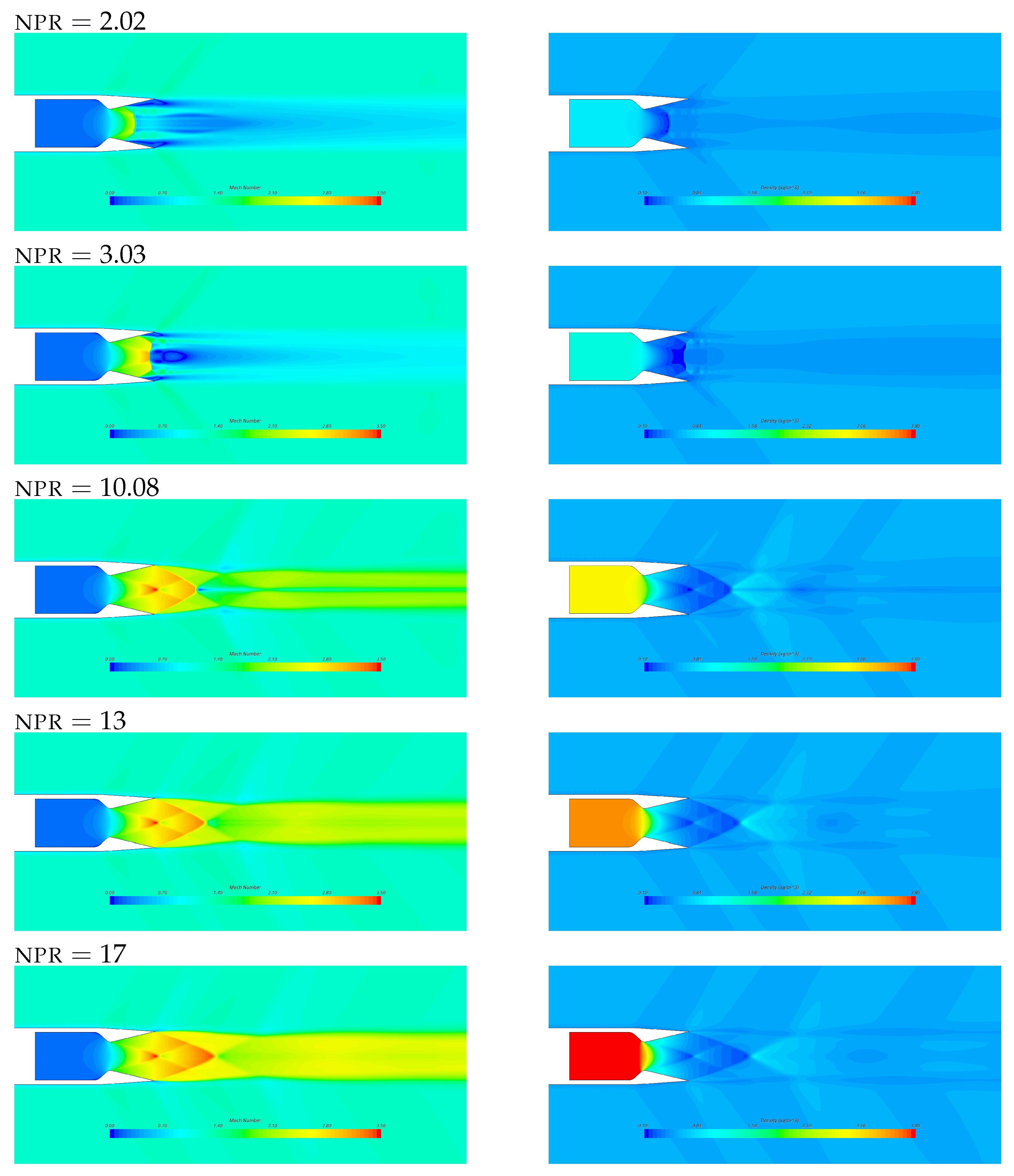
Figure 9.
Internal nozzle walls static pressure distribution (a–c), and boat-tail pressure coefficient distribution (d–f). Comparison with experimental data.
Figure 9.
Internal nozzle walls static pressure distribution (a–c), and boat-tail pressure coefficient distribution (d–f). Comparison with experimental data.
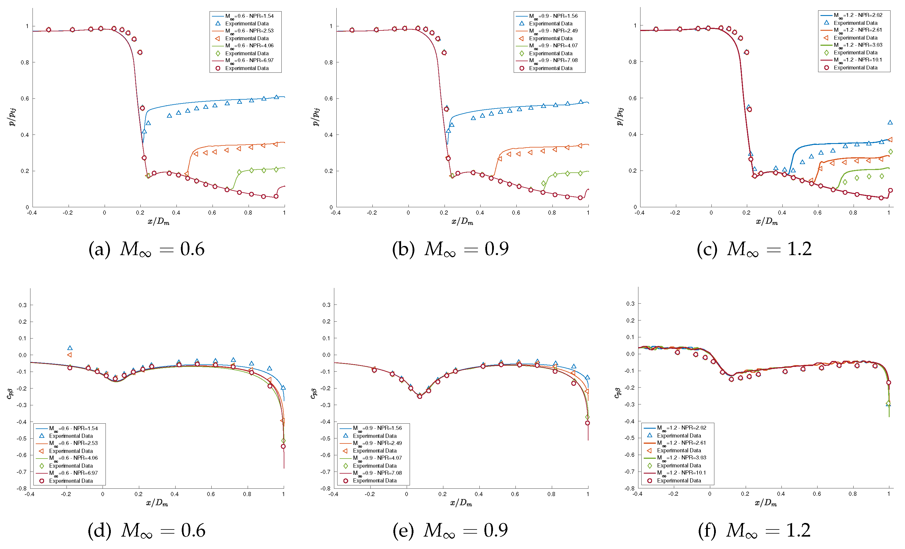
Figure 10.
Mesh detail close to the injection zone.

Figure 11.
Mach number (left) and density (right) fields for axisymmetric injection at different positions in the nozzle divergent.
Figure 11.
Mach number (left) and density (right) fields for axisymmetric injection at different positions in the nozzle divergent.

Figure 12.
Comparison between the axisymmetric (a) and three dimensional (b) solution of the simulation with secondary injection.
Figure 12.
Comparison between the axisymmetric (a) and three dimensional (b) solution of the simulation with secondary injection.
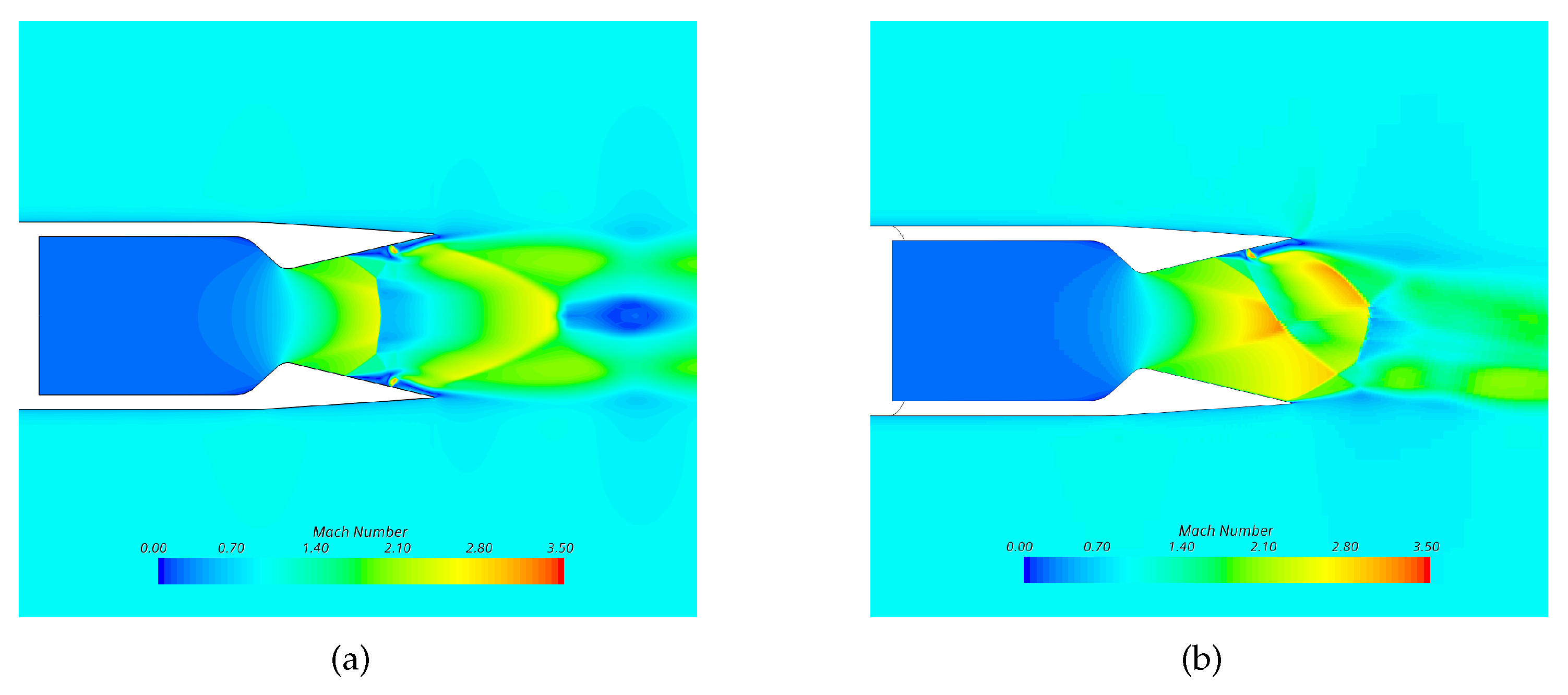
Figure 13.
Three-dimensional (3D) mesh configuration: global view and nozzle detail.

Figure 14.
Diagram of pitch thrust-vector angle against the secondary mass-flow rate, smf.

Figure 15.
Wall pressure distribution at different secondary mass-flow injections rates (smf).

Figure 16.
Flowfield in the nozzle symmetry-plane. Mach contour at different secondary mass-flow injection rates (smf).
Figure 16.
Flowfield in the nozzle symmetry-plane. Mach contour at different secondary mass-flow injection rates (smf).
Publisher’s Note: MDPI stays neutral with regard to jurisdictional claims in published maps and institutional affiliations. |
© 2021 by the authors. Licensee MDPI, Basel, Switzerland. This article is an open access article distributed under the terms and conditions of the Creative Commons Attribution (CC BY) license (https://creativecommons.org/licenses/by/4.0/).
Share and Cite
MDPI and ACS Style
Resta, E.; Marsilio, R.; Ferlauto, M. Thrust Vectoring of a Fixed Axisymmetric Supersonic Nozzle Using the Shock-Vector Control Method. Fluids 2021, 6, 441. https://doi.org/10.3390/fluids6120441
AMA Style
Resta E, Marsilio R, Ferlauto M. Thrust Vectoring of a Fixed Axisymmetric Supersonic Nozzle Using the Shock-Vector Control Method. Fluids. 2021; 6(12):441. https://doi.org/10.3390/fluids6120441
Chicago/Turabian StyleResta, Emanuele, Roberto Marsilio, and Michele Ferlauto. 2021. "Thrust Vectoring of a Fixed Axisymmetric Supersonic Nozzle Using the Shock-Vector Control Method" Fluids 6, no. 12: 441. https://doi.org/10.3390/fluids6120441