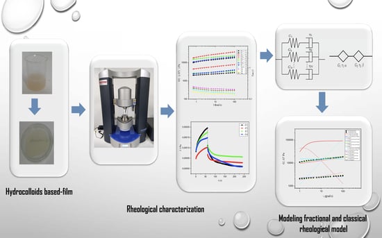
Characterization and Modeling of the Viscoelastic Behavior of Hydrocolloid-Based Films Using Classical and Fractional Rheological Models

Abstract

Hydrocolloid-based films are a good alternative in the development of biodegradable films due to their properties, such as non-toxicity, functionality, and biodegradability, among others. In this work, films based on hydrocolloids (gellan gum, carrageenan, and guar gum) were formulated, evaluating their dynamic rheological behavior and creep and recovery. Maxwell’s classical and fractional rheological models were implemented to describe its viscoelastic behavior, using the Vortex Search Algorithm for the estimation of the parameters. The hydrocolloid-based films showed a viscoelastic behavior, where the behavior of the storage modulus $({\mathrm{G}}^{\prime })$ and loss modulus (${\mathrm{G}}^{″})$ indicated a greater elastic behavior (${\mathrm{G}}^{\prime }>{\mathrm{G}}^{″}$). The Maxwell fractional model with two spring-pots showed an optimal fit of the experimental data of storage modulus (${\mathrm{G}}^{\prime }$) and loss modulus (${\mathrm{G}}^{″})$ and a creep compliance (J) (${\mathrm{F}}_{\min }<0.1$ and ${\mathrm{R}}^2>0.98$). This shows that fractional models are an excellent alternative for describing the dynamic rheological behavior and creep recovery of films. These results show the importance of estimating parameters that allow for the dynamic rheological and creep behaviors of hydrocolloid-based films for applications in the design of active films because they allow us to understand their behavior from a rheological point of view, which can contribute to the design and improvement of products such as food coatings, food packaging, or other applications containing biopolymers.

1. Introduction

Recently, the development of edible food packaging and biodegradable films from natural polymeric materials has attracted the attention of researchers due to environmental pollution caused by the use of conventional non-biodegradable plastic [1]. The functionality of edible films has been improved and diversified through the development of different film formulations, and knowledge about them has continuously increased due to worldwide research on their properties [2]. In general, polysaccharides, such as pectin, starch, cellulose, alginates, and other hydrocolloids, have a good performance in film-forming due to their chemical nature [2,3]. The addition of a plasticizer, such as glycerol or sorbitol, increases the mobility of polymer chains because they reduce intermolecular forces, improving the flexibility and extensibility of the film [3,4]. The edible films can be obtained from edible materials through two different methods: wet and dry processes, also called solvent casting and extrusion processes, respectively. The casting method (also called solvent casting) is the most commonly used method for film formation on laboratory and pilot scales and its main advantage is an ease of manufacturing without the usage of low-cost specialized equipment [5]. Hydrocolloids, particularly gellan gum, carrageenan, and guar gum, are biodegradable and non-toxic products based on renewable resources. Gellan gum is composed of repeating tetrasaccharide (1,3-β-D-glucose, 1, 4-β-d-glucuronic acid, 1, 4-β-D-glucose, and 1, 4-α-l-rhamnose) units containing one carboxyl side group. It is used as a gelling agent and occurs in two steps with the addition of salts or acids. In the first step, double helices form during cooling, and in the second step, this is followed by a cation-mediated aggregation of the double helices that leads to gelation. The gelation conditions bring about a wide variety of textures and mechanical properties. This extends the application of gellan gum to many fields, such as biomedicine, pharmacology, and the food industry [6,7,8,9,10]. Carrageenan is a natural sulfated polysaccharide that is extracted from Rhodophyceae seaweed and consists of a disaccharide repeating unit of alternating α-(1–3)-D-galactose and β-(1–4)-3,6-anhydro-D-galactose [11]. Variation in the derivatives and position of carrageenan sulfates can alter the rheological properties of gels in food applications [12], but kappa carrageenan and iota carrageenan are the most common types used in the industry due to their good gelling properties [13].

Blending two or more different hydrocolloids can change both the physical and rheological properties of film-forming solutions and, consequently, of films, strongly. These changes occur due to compatibility/incompatibility between two macromolecules, which depend on their molecular weights, chemical structures, conformations, and hydration behaviors, as well as the addition of various chemicals or additives [14,15].

The rheological characterization of foods provides important information for food scientists, namely, ingredient selection strategies to design, improve, and optimize their products, to select and optimize their manufacturing processes, and to design packaging and storage strategies [16]. As a complex matrix, food generally cannot be described by an ideal model, such as an ideal liquid, if the matrix is viscous, or an ideal solid, if it is elastic, nor as an ideal plastic, a state between liquid and solid. To determine and quantify the viscoelastic behavior of a matrix, quasi-static (transient) and dynamic tests can be carried out [2]. To describe the viscoelastic nature of food products, rheological models based on mechanical analogues consisting of spring elements (elastic behaviour) and dash-pot elements (viscous behaviour) are used [17,18,19]. Different combinations of spring and dash-pot elements represent different constitutive rheological models [20].

The main limitation of the classical models, such as generalized Maxwell models, is that these require many parameters to get the best fit with the experimental data [19]. Furthermore, more elements of the rheological model mean that more parameters must be evaluated, increasing the complexity of associating the numerical values of the coefficients with the viscoelastic and textural properties of the materials [20], making it difficult to understand the physical importance of all parameters found in the classical models [21]. As an alternative approach, fractional calculus has been an empirical method of analyzing the linear viscoelastic response of polymeric materials [22,23], food products, and ingredients such as fruits, vegetables, gums, and emulsifiers [20,24,25,26] in an increasing number of research articles. By this approach, the capacity of conventional viscoelastic models can be enhanced, and their well-known limitations can be overcome, while a satisfactory description of viscoelastic response can be obtained by a reduced number of model parameters [23].

The objective of this work was to develop films based on hydrocolloids, evaluate, and describe their viscoelastic behavior (dynamic rheological and creep recovery) using classic and fractional rheological models with a new metaheuristic approach to estimate their parameters. Previous studies have implemented metaheuristic algorithms, such as Genetic Algorithms (GA), to estimate the parameters of fractional rheological models [27,28,29]. In this study, we propose the application of the Vortex Search Algorithm (VSA) for the estimation of the parameters of the proposed rheological models, such as the generalized Maxwell and Kelvin models and the fractional Maxwell and Kelvin models, with one and two spring-pots.

2. Materials and Methods

2.1. Material

Gellan gum, carrageenan, and guar gum was supplied by Química Aromática Andina SAS (Medellin, Colombia), Tecnas S.A (Medellin, Colombia) and ABC Laboratories (Bogota, Colombia) respectively. Glycerol, sorbitol, potassium chloride, and calcium chloride were supplied by ABC Laboratories (Bogota, Colombia).

2.2. Film Preparation

The hydrocolloid-based films were prepared from a mixture of guar gum, gellan gum and carrageenan with a solution-casting technique. A simple mixture design was used, as shown in

Table 1. Sample code and formulation of hydrocolloid-based film.

Sample Code	Gellan Gum (%)	Carrageenan (%)	Potassium Citrate (%)	Calcium Chloride (%)
F1	0.25	1.35	0.2	0.4
F2	0.25	1.35	0.4	0.2
F3	0.4	1.2	0.2	0.4
F4	0.4	1.2	0.4	0.2

. The film preparation procedures are described as follows: guar gum, gellan gum, and carrageenan were dissolved in 80 mL of distilled water with the addition of potassium citrate and calcium chloride. This mixture was heated to 80 °C for 15 min under constant agitation. Guar gum was added with a concentration of 0.8% p/v. A mixture of plasticizers (sorbitol and glycerol) was used, which were added with a concentration of 6% p/v into the hydrocolloid solution film. The mixture was then stirred for 15 min at 85 °C and the resulting suspension was casted in a Petri dish. These samples were dried for 36 h at room temperature.

2.3. Viscoelastic Tests

The viscoelastic characterization of the samples’ films was analyzed using a HAAKE MARS Modular Advanced Rheometer System 60 with Peltier and the geometry of a rough dish of 35 mm diameter with 0.3 mm gap was used. Stress sweeps were carried out at a frequency of 1 Hz, applying an ascending series of stress values from 0.1 to 100 Pa for the determination of the linear viscoelasticity interval.

2.3.1. Dynamic Rheological Tests

Oscillatory shear tests were performed to obtain the viscoelastic response of the material. Frequency sweeps were performed to obtain the mechanical spectrum by applying a stress value, within the linear viscoelastic range, in an angular frequency range comprising between 10⁻¹ and 10² rad/s. The tests were carried out at 30 °C. The obtained viscoelastic parameters were storage modulus (${\mathrm{G}}^{\prime }$), loss modulus (${\mathrm{G}}^{″}$), and tan ($\mathsf{\delta }$).

2.3.2. Creep and Recovery Tests

Creep and recovery tests were performed to determine the values of compliance in the creep and recovery phases. Creep and recovery analyses of hydrocolloid films were performed at 30 °C for each sample. In the creep phase, hydrocolloid film samples were subjected to constant stress for 60 s. In the recovery phase, the applied stress was suddenly removed, and the sample was analyzed for recoverable shear for 240 s.

3. Rheological Model

Viscoelastic models can be used to represent rate-dependent behaviors [30], where the stress-strain relation is a function of the rate of strain, and the creep compliance $\mathrm{J}$ behavior, where the strain increases under a constant applied load. When the material is subjected to harmonic stress or strain, another important part of the theory of viscoelasticity is the useful concept [31] of the complex modulus ${\mathrm{G}}^{*}$, where the real part, ${\mathrm{G}}^{\prime }$, of this modulus is associated with the amount of energy stored in the element during a complete loading cycle and is called the storage modulus. The imaginary part, ${\mathrm{G}}^{″}$, relates to the energy dissipated per cycle and is called the loss modulus [32].

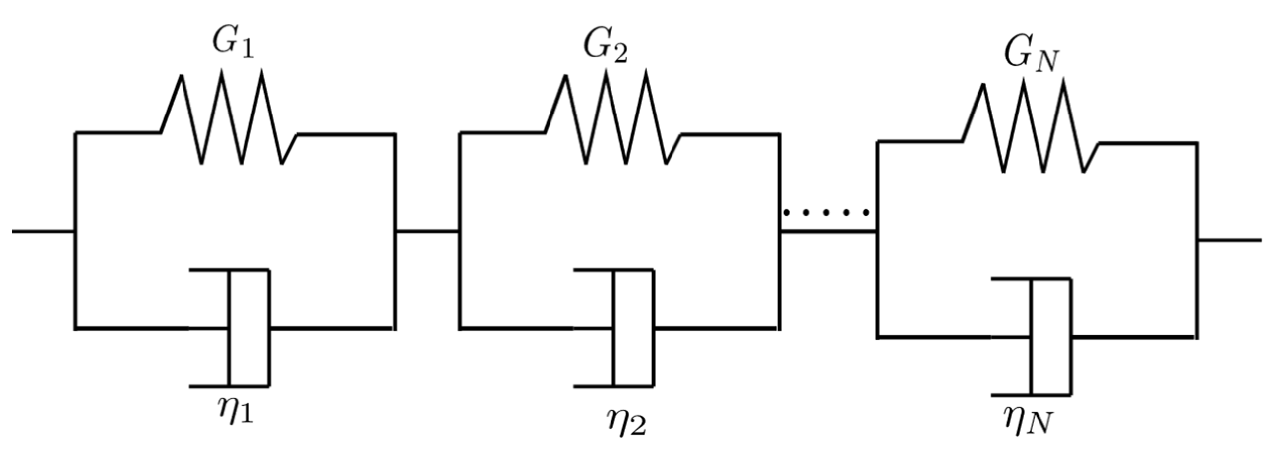
3.1. The Generalized Maxwell Model

The generalized Maxwell model is a typical classic viscoelastic model composed of multiple Maxwell elements connected in parallel, as shown in Figure 1 [33].

The constitutive equation for generalized Maxwell model can be expressed in the general form:

$${\displaystyle \sum }_{\mathrm{n}=0}^{\mathrm{N}}{\mathrm{a}}_{\mathrm{n}}\frac{{\mathrm{d}}^{\mathrm{n}}\mathsf{\sigma }\left(\mathrm{t}\right)}{{\mathrm{dt}}^{\mathrm{n}}}={\displaystyle \sum }_{\mathrm{m}=0}^{\mathrm{M}}{\mathrm{b}}_{\mathrm{n}}\frac{{\mathrm{d}}^{\mathrm{m}}\mathsf{\gamma }\left(\mathrm{t}\right)}{{\mathrm{dt}}^{\mathrm{m}}}$$

(1)

where $\mathrm{N}=\mathrm{M}$ and ${\mathrm{b}}_0=0$. For $\mathrm{N}=1$, Equation (1) is expressed as follows:

$$\mathsf{\sigma }\mathrm{t}+\mathsf{\tau }\frac{\mathrm{d}\mathsf{\sigma }\left(\mathrm{t}\right)}{\mathrm{dt}}={\mathrm{G}}_1\frac{\mathrm{d}\mathsf{\epsilon }\left(\mathrm{t}\right)}{\mathrm{dt}}$$

(2)

where ${\mathrm{G}}_1$ is the elastic modulus in Pa, $\mathsf{\tau }$ is the characteristic time in seconds, given by the following expression $\mathsf{\tau }=\raisebox{1ex}{${\mathsf{\eta }}_1$}\!\left/ \!\raisebox{-1ex}{${\mathrm{G}}_1$}\right.$, ${\mathsf{\eta }}_1$ being the viscosity in Pa seconds. The complex modulus can be derived by transforming Equation (1) into the frequency domain. Applying the Fourier transformation to Equation (1), considering that

$$\mathrm{ℱ}\left\{\frac{\mathrm{d}}{\mathrm{dt}}\mathrm{f}\left(\mathrm{t}\right)\right\}=(\mathrm{i}\mathsf{\omega })\tilde{\mathrm{f}}(\mathsf{\omega }),$$

(3)

we obtain the following:

$${\mathrm{G}}^{\ast }\left(\mathsf{\omega }\right)=\frac{\tilde{\mathsf{\sigma }}\left(\mathsf{\omega }\right)}{\tilde{\mathsf{\epsilon }}\left(\mathsf{\omega }\right)}=\frac{{\mathrm{G}}_1\mathsf{\tau }\mathsf{\omega }\mathrm{i}}{1+\mathsf{\tau }\mathsf{\omega }\mathrm{i}}$$

(4)

where ${\mathrm{G}}^{\ast }\left(\mathsf{\omega }\right)$ is the complex modulus. Separating the real and imaginary parts, we can obtain the storage and loss modulus, respectively:

$$\begin{gathered} {\mathrm{G}}^{\prime }\left(\mathsf{\omega }\right)=\frac{{\mathrm{G}}_1{(\mathsf{\tau }\mathsf{\omega })}^2}{1+{(\mathsf{\tau }\mathsf{\omega })}^2} \\ {\mathrm{G}}^{″}\left(\mathsf{\omega }\right)=\frac{{\mathrm{G}}_1\mathsf{\tau }\mathsf{\omega }}{1+{(\mathsf{\tau }\mathsf{\omega })}^2} \end{gathered}$$

(5)

The creep compliance J is obtained by applying the Laplace transformation to Equation (1), obtaining:

$$\mathrm{J}(\mathrm{s})=\frac{\mathsf{\epsilon }(\mathrm{s})}{\mathrm{s} \mathsf{\sigma }(\mathrm{s})}=\frac{1}{{\mathrm{G}}_1}\left(\frac{1}{\mathrm{s}}+\frac{1}{\mathsf{\tau }{\mathrm{s}}^2}\right)$$

(6)

Applying the inverse Laplace transformation, we obtain:

$$\mathrm{J}(\mathrm{t})=\frac{1}{{\mathrm{G}}_1}\left(1+\frac{\mathrm{t}}{\mathsf{\tau }}\right)$$

(7)

Now, for N = 2, Equation (1) is expressed as follows:

$$\mathsf{\sigma }\mathrm{t}+({\mathsf{\tau }}_{1+}{\mathsf{\tau }}_2)\frac{\mathrm{d}\mathsf{\sigma }\left(\mathrm{t}\right)}{\mathrm{dt}}+{\mathsf{\tau }}_1{\mathsf{\tau }}_2\frac{{\mathrm{d}\mathsf{\sigma }}^2\left(\mathrm{t}\right)}{{\mathrm{dt}}^2}=({\mathrm{G}}_1{\mathsf{\tau }}_1+{\mathrm{G}}_2{\mathsf{\tau }}_2)\frac{\mathrm{d}\mathsf{\epsilon }\left(\mathrm{t}\right)}{\mathrm{dt}}+({\mathrm{G}}_1+{\mathrm{G}}_2)\frac{{\mathrm{d}\mathsf{\epsilon }}^2\left(\mathrm{t}\right)}{{\mathrm{dt}}^2}$$

(8)

where ${\mathrm{G}}_1$ and ${\mathrm{G}}_2$ are elastic modules corresponding to Maxwell elements connected in parallel in Pa, ${\mathsf{\tau }}_1 \mathrm{and} {\mathsf{\tau }}_2$ are the characteristics’ times in seconds, given by the following expression ${\mathsf{\tau }}_1=\raisebox{1ex}{${\mathsf{\eta }}_1$}\!\left/ \!\raisebox{-1ex}{${\mathrm{G}}_1$}\right.$ and ${\mathsf{\tau }}_2=\raisebox{1ex}{${\mathsf{\eta }}_2$}\!\left/ \!\raisebox{-1ex}{${\mathrm{G}}_2$}\right.$, being ${\mathsf{\eta }}_1$ and ${\mathsf{\eta }}_2$ are viscosities in Pa seconds. The complex modulus can be derived applying Equations (3)–(8), obtaining:

$${\mathrm{G}}^{\ast }\left(\mathsf{\omega }\right)=\frac{\tilde{\mathsf{\sigma }}\left(\mathsf{\omega }\right)}{\tilde{\mathsf{\epsilon }}\left(\mathsf{\omega }\right)}=\frac{{\mathrm{G}}_1{\mathsf{\tau }}_1\mathsf{\omega }\mathrm{i}}{1+{\mathsf{\tau }}_2\mathsf{\omega }\mathrm{i}}+\frac{{\mathrm{G}}_2{\mathsf{\tau }}_2\mathsf{\omega }\mathrm{i}}{1+{\mathsf{\tau }}_2\mathsf{\omega }\mathrm{i}}$$

(9)

Separating the real and imaginary parts, we can obtain the storage and loss modulus, respectively:

$$\begin{gathered} {\mathrm{G}}^{\prime }\left(\mathsf{\omega }\right)=\frac{{\mathrm{G}}_1{({\mathsf{\tau }}_1\mathsf{\omega })}^2}{1+{({\mathsf{\tau }}_1\mathsf{\omega })}^2}+\frac{{\mathrm{G}}_2{({\mathsf{\tau }}_2\mathsf{\omega })}^2}{1+{({\mathsf{\tau }}_2\mathsf{\omega })}^2} \\ {\mathrm{G}}^{″}\left(\mathsf{\omega }\right)=\frac{{\mathrm{G}}_1{\mathsf{\tau }}_1\mathsf{\omega }}{1+{({\mathsf{\tau }}_1\mathsf{\omega })}^2}+\frac{{\mathrm{G}}_2{\mathsf{\tau }}_2\mathsf{\omega }}{1+{({\mathsf{\tau }}_2\mathsf{\omega })}^2} \end{gathered}$$

(10)

The creep compliance J is obtained by applying the Laplace transformation to Equation (8) and then the inverse Laplace transformation to obtain the following:

$$\mathrm{J}\left(\mathrm{t}\right)=\left(\frac{1}{{\mathrm{G}}_1+{\mathrm{G}}_2}\right){\mathrm{e}}^{\raisebox{1ex}{$-\mathrm{t}$}\!\left/ \!\raisebox{-1ex}{${\mathsf{\tau }}_{\mathrm{r}}$}\right.}+\left(\frac{{\mathsf{\tau }}_1+{\mathsf{\tau }}_2-{\mathsf{\tau }}_{\mathrm{r}}}{{\mathsf{\tau }}_1{\mathrm{G}}_1+{\mathsf{\tau }}_2{\mathrm{G}}_2}\right)\left(1-{\mathrm{e}}^{\raisebox{1ex}{$-\mathrm{t}$}\!\left/ \!\raisebox{-1ex}{${\mathsf{\tau }}_{\mathrm{r}}$}\right.}\right)+\frac{\mathrm{t}}{{\mathsf{\tau }}_1{\mathrm{G}}_1+{\mathsf{\tau }}_2{\mathrm{G}}_2}$$

(11)

where ${\mathsf{\tau }}_{\mathrm{r}}=\raisebox{1ex}{${\mathsf{\tau }}_1{\mathsf{\tau }}_2\left({\mathrm{G}}_1+{\mathrm{G}}_2\right)$}\!\left/ \!\raisebox{-1ex}{$({\mathsf{\tau }}_1{\mathrm{G}}_1+{\mathsf{\tau }}_2{\mathrm{G}}_2)$}\right.$.

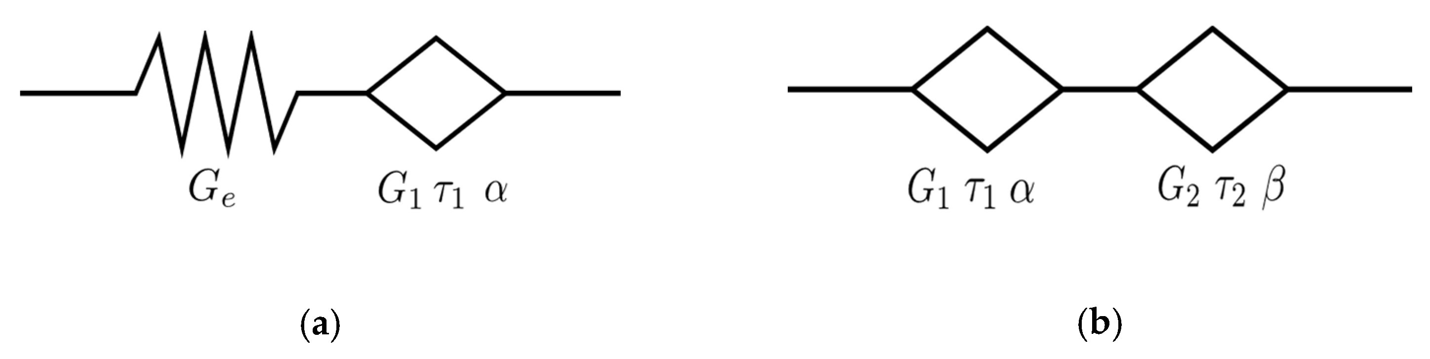
3.2. The Fractional Maxwell Model

The fractional Maxwell model with one spring-pot consists of a spring connected in series with one spring-pot. In this model, the dash-pots of the conventional Maxwell model have been replaced with a Scott-Blair element, as shown in Figure 2a.

The constitutive equation is given by:

$$\begin{array}{r}\hfill \mathsf{\sigma }\left(\mathrm{t}\right)+{\mathsf{\tau }}^{\mathsf{\alpha }}\frac{{\mathrm{d}}^{\mathsf{\alpha }}\mathsf{\sigma }\left(\mathrm{t}\right)}{{\mathrm{dt}}^{\mathsf{\alpha }}}={\mathrm{G}}_{\mathrm{e}}{\mathsf{\tau }}^{\mathsf{\alpha }}\frac{{\mathrm{d}}^{\mathsf{\alpha }}\mathsf{\epsilon }\left(\mathrm{t}\right)}{{\mathrm{dt}}^{\mathsf{\alpha }}}\end{array}$$

(12)

where $\mathsf{\alpha }$ is fractional exponents (0 < α < 1), ${\mathrm{G}}_{\mathrm{e}}$ is the elastic modulus, $\mathsf{\tau }$ is the characteristic time, given by the following expression ${\mathsf{\tau }}^{\mathsf{\alpha }}=\raisebox{1ex}{${\mathrm{G}}_1{\mathsf{\tau }}_1$}\!\left/ \!\raisebox{-1ex}{${\mathrm{G}}_{\mathrm{e}}$}\right.$. The fractional derivative of order $0<\mathsf{\alpha }<1$ is defined according to the Caputo definition as [25]:

$$\begin{array}{r}\hfill {\mathrm{D}}_{\mathrm{t}}^{\mathsf{\alpha }}\mathrm{f}\left(\mathrm{t}\right)=\frac{1}{\Gamma \left(1-\mathsf{\alpha }\right)}{{\displaystyle \int }}_0^{\mathrm{t}}\frac{\mathrm{df}\left(\mathsf{\tau }\right)}{\mathrm{dt}}{(\mathrm{t}-\mathsf{\tau })}^{-\mathsf{\alpha }}\mathrm{d}\mathsf{\tau }\end{array}$$

(13)

where $\Gamma (1-\mathsf{\alpha })$ denotes the Euler Gamma function. According to the fractional differential Fourier transformation [34]:

$$\begin{array}{r}\hfill ℱ\left\{\frac{{\mathrm{d}}^{\mathsf{\alpha }}}{{\mathrm{d}}^{\mathsf{\alpha }}}\mathrm{f}\left(\mathrm{t}\right)\right\}={(\mathrm{i}\mathsf{\omega })}^{\mathsf{\alpha }}\tilde{\mathrm{f}}\left(\mathsf{\omega }\right)\end{array}$$

(14)

where $\tilde{\mathrm{f}}\left(\mathsf{\omega }\right)=ℱ\{\mathrm{f}\left(\mathrm{t}\right);\mathsf{\omega }\}$ [35], the complex modulus of the model can be derived applying Equations (12)–(14), obtaining:

$$\begin{array}{r}\hfill {\mathrm{G}}^{*}\left(\mathsf{\omega }\right)=\frac{\tilde{\mathsf{\sigma }}\left(\mathsf{\omega }\right)}{\tilde{\mathsf{\epsilon }}\left(\mathsf{\omega }\right)}=\frac{{\mathrm{G}}_{\mathrm{e}}{(\mathrm{i}\mathsf{\tau }\mathsf{\omega })}^{\mathsf{\alpha }}}{1+{(\mathrm{i}\mathsf{\tau }\mathsf{\omega })}^{\mathsf{\alpha }}}\end{array}$$

(15)

Separating the real and imaginary parts, we can obtain the storage modulus and loss modulus:

$$\begin{gathered} {\mathrm{G}}^{\prime }\left(\mathsf{\omega }\right)={\mathrm{G}}_{\mathrm{e}}\frac{{(\mathsf{\omega }\mathsf{\tau })}^{2\mathsf{\alpha }}+{(\mathsf{\omega }\mathsf{\tau })}^{\mathsf{\alpha }}\cos \left(\mathsf{\pi }\mathsf{\alpha }/2\right)}{1+2{(\mathsf{\omega }\mathsf{\tau })}^{\mathsf{\alpha }}\cos \left(\mathsf{\pi }\mathsf{\alpha }/2\right)+{(\mathsf{\omega }\mathsf{\tau })}^{2\mathsf{\alpha }}} \\ {\mathrm{G}}^{″}\left(\mathsf{\omega }\right)={\mathrm{G}}_{\mathrm{e}}\frac{{(\mathsf{\omega }\mathsf{\tau })}^{\mathsf{\alpha }}\sin \left(\mathsf{\pi }\mathsf{\alpha }/2\right)}{1+2{(\mathsf{\omega }\mathsf{\tau })}^{\mathsf{\alpha }}\cos \left(\mathsf{\pi }\mathsf{\alpha }/2\right)+{(\mathsf{\omega }\mathsf{\tau })}^{2\mathsf{\alpha }}} \end{gathered}$$

(16)

The creep compliance is obtained by applying the Laplace transform to Equation (12),

$$\begin{array}{r}\hfill \mathrm{J}\left(\mathrm{s}\right)=\frac{\mathsf{\epsilon }\left(\mathrm{s}\right)}{\mathrm{s}\mathsf{\sigma }\left(\mathrm{s}\right)}=\frac{1}{{\mathrm{G}}_{\mathrm{e}}}\left(\frac{1}{\mathrm{s}}+\frac{{\mathrm{s}}^{-\mathsf{\alpha }-1}}{{\mathsf{\tau }}^{\mathsf{\alpha }}}\right)\end{array}$$

(17)

Applying the inverse Laplace transformation, we obtain:

$$\begin{array}{r}\hfill \mathrm{J}\left(\mathrm{t}\right)=\frac{1}{{\mathrm{G}}_{\mathrm{e}}}+\frac{{\left(\raisebox{1ex}{$\mathrm{t}$}\!\left/ \!\raisebox{-1ex}{$\mathsf{\tau }$}\right.\right)}^{\mathsf{\alpha }}}{{\mathrm{G}}_{\mathrm{e}}\Gamma \left(\mathsf{\alpha }+1\right)}\end{array}$$

(18)

The Maxwell fractional model with two spring-pots consists of two Scott-Blair elements or spring-pots connected in series, as shown in Figure 2b. The constitutive equation is given by:

$$\begin{array}{r}\hfill \mathsf{\sigma }\left(\mathrm{t}\right)+{\mathsf{\tau }}^{\mathsf{\alpha }-\mathsf{\beta }}\frac{{\mathrm{d}}^{\mathsf{\alpha }-\mathsf{\beta }}\mathsf{\sigma }\left(\mathrm{t}\right)}{{\mathrm{dt}}^{\mathsf{\alpha }-\mathsf{\beta }}}={\mathrm{G}}^{{\mathsf{\tau }}^{\mathsf{\alpha }}}\frac{{\mathrm{d}}^{\mathsf{\alpha }}\mathsf{\epsilon }\left(\mathrm{t}\right)}{{\mathrm{dt}}^{\mathsf{\alpha }}}\end{array}$$

(19)

where $\mathrm{G}$ is an elastic modulus in Pa given by the following expression, $\mathrm{G}={\mathrm{G}}_1{\left(\frac{{\mathsf{\tau }}_1}{\mathsf{\tau }}\right)}^{\mathsf{\alpha }},$ and $\mathsf{\tau }$ is the characteristic time of the model in seconds, defined by the following expression: $\mathsf{\tau }={\left(\raisebox{1ex}{${\mathrm{G}}_1{\mathsf{\tau }}_1^{\mathsf{\alpha }}$}\!\left/ \!\raisebox{-1ex}{${\mathrm{G}}_2{\mathsf{\tau }}_2^{\mathsf{\beta }}$}\right.\right)}^{\raisebox{1ex}{$1$}\!\left/ \!\raisebox{-1ex}{$\mathsf{\alpha }-\mathsf{\beta }$}\right.}$. In Equation (19), we assumed $\mathsf{\alpha }>\mathsf{\beta }$ without a loss of generality [36]. Applying the Fourier transformation to Equation (19), we obtain:

$$\begin{array}{r}\hfill {\mathrm{G}}^{*}\left(\mathsf{\omega }\right)=\frac{\tilde{\mathsf{\sigma }}\left(\mathsf{\omega }\right)}{\tilde{\mathsf{\epsilon }}\left(\mathsf{\omega }\right)}=\mathrm{G}\frac{{(\mathrm{i}\mathsf{\tau }\mathsf{\omega })}^{\mathsf{\alpha }}}{1+{(\mathrm{i}\mathsf{\tau }\mathsf{\omega })}^{\mathsf{\alpha }-\mathsf{\beta }}}\end{array}$$

(20)

where ${\mathrm{G}}^{\ast }\left(\mathsf{\omega }\right)$ is the complex modulus. Separating the real and imaginary parts, we can obtain the storage and loss modulus, respectively:

$$\begin{gathered} {\mathrm{G}}^{\prime }\left(\mathsf{\omega }\right)=\mathrm{G}\frac{{(\mathsf{\omega }\mathsf{\tau })}^{\mathsf{\alpha }}\cos \left(\mathsf{\pi }\mathsf{\alpha }/2\right)+{(\mathsf{\omega }\mathsf{\tau })}^{2\mathsf{\alpha }-\mathsf{\beta }}\cos \left(\mathsf{\pi }\mathsf{\beta }/2\right)}{1+2{(\mathsf{\omega }\mathsf{\tau })}^{\mathsf{\alpha }-\mathsf{\beta }}\cos \left(\mathsf{\pi }\left(\mathsf{\alpha }-\mathsf{\beta }\right)/2\right)+{(\mathsf{\omega }\mathsf{\tau })}^{2\left(\mathsf{\alpha }-\mathsf{\beta }\right)}} \\ {\mathrm{G}}^{″}\left(\mathsf{\omega }\right)=\mathrm{G}\frac{{(\mathsf{\omega }\mathsf{\tau })}^{\mathsf{\alpha }}\sin \left(\mathsf{\pi }\mathsf{\alpha }/2\right)+{(\mathsf{\omega }\mathsf{\tau })}^{2\mathsf{\alpha }-\mathsf{\beta }}\sin \left(\mathsf{\pi }\mathsf{\beta }/2\right)}{1+2{(\mathsf{\omega }\mathsf{\tau })}^{\mathsf{\alpha }-\mathsf{\beta }}\cos \left(\mathsf{\pi }\left(\mathsf{\alpha }-\mathsf{\beta }\right)/2\right)+{(\mathsf{\omega }\mathsf{\tau })}^{2\left(\mathsf{\alpha }-\mathsf{\beta }\right)}} \end{gathered}$$

(21)

The creep compliance is obtained by applying the Laplace transform to Equation (37), obtaining:

$$\begin{array}{r}\hfill \mathrm{J}\left(\mathrm{s}\right)=\frac{\mathsf{\epsilon }\left(\mathrm{s}\right)}{\mathrm{s}\mathsf{\sigma }\left(\mathrm{s}\right)}=\frac{1}{\mathrm{G}}\left(\frac{{\mathrm{s}}^{-\mathsf{\alpha }-1}}{{\mathsf{\tau }}^{\mathsf{\alpha }}}+\frac{{\mathrm{s}}^{-\mathsf{\beta }-1}}{{\mathsf{\tau }}^{\mathsf{\beta }}}\right)\end{array}$$

(22)

Applying the inverse Laplace transformation, we obtain:

$$\begin{array}{r}\hfill \mathrm{J}\left(\mathrm{t}\right)=\frac{{\left(\raisebox{1ex}{$\mathrm{t}$}\!\left/ \!\raisebox{-1ex}{$\mathsf{\tau }$}\right.\right)}^{\mathsf{\alpha }}}{\mathrm{G}\Gamma \left(\mathsf{\alpha }+1\right)}+\frac{{\left(\raisebox{1ex}{$\mathrm{t}$}\!\left/ \!\raisebox{-1ex}{$\mathsf{\tau }$}\right.\right)}^{\mathsf{\beta }}}{\mathrm{G}\Gamma \left(\mathsf{\beta }+1\right)}\end{array}$$

(23)

3.3. The Generalized Kelvin Model

The generalized Kelvin model is a typical classic viscoelastic model composed of multiple Kelvin elements connected in series, as shown in Figure 3.

The constitutive equation for the generalized Kelvin model can be expressed in the general form:

$${\displaystyle \sum }_{\mathrm{m}=0}^{\mathrm{M}}{\mathrm{a}}_{\mathrm{m}}\frac{{\mathrm{d}}^{\mathrm{m}}\mathsf{\sigma }\left(\mathrm{t}\right)}{{\mathrm{dt}}^{\mathrm{m}}}={\displaystyle \sum }_{\mathrm{n}=0}^{\mathrm{N}}{\mathrm{b}}_{\mathrm{n}}\frac{{\mathrm{d}}^{\mathrm{n}}\mathsf{\epsilon }\left(\mathrm{t}\right)}{{\mathrm{dt}}^{\mathrm{n}}}$$

(24)

where $\mathrm{M}=\mathrm{N}-1$ and ${\mathrm{a}}_0=1$. For $\mathrm{N}=1$, Equation (24) is expressed as follows:

$$\mathsf{\sigma }(\mathrm{t})={\mathrm{G}}_1\mathsf{\epsilon }(\mathrm{t})+{\mathrm{G}}_1\mathsf{\tau }\frac{\mathrm{d}\mathsf{\epsilon }\left(\mathrm{t}\right)}{\mathrm{dt}}$$

(25)

where ${\mathrm{G}}_1$ is the elastic modulus in Pa, $\mathsf{\tau }$ is the retardation time in seconds, given by the following expression $\mathsf{\tau }=\raisebox{1ex}{${\mathsf{\eta }}_1$}\!\left/ \!\raisebox{-1ex}{${\mathrm{G}}_1$}\right.$, being ${\mathsf{\eta }}_1$ the viscosity in Pa seconds. The complex modulus can be derived applying (3) to (25), obtaining the following:

$${\mathrm{G}}^{\ast }\left(\mathsf{\omega }\right)=\frac{\tilde{\mathsf{\sigma }}\left(\mathsf{\omega }\right)}{\tilde{\mathsf{\epsilon }}\left(\mathsf{\omega }\right)}={\mathrm{G}}_1(1+\mathsf{\tau }\mathsf{\omega }\mathrm{i})$$

(26)

Separating the real and imaginary parts, we can obtain the storage modulus and loss modulus, respectively:

$$\begin{gathered} {\mathrm{G}}^{\prime }\left(\mathsf{\omega }\right)={\mathrm{G}}_1 \\ {\mathrm{G}}^{″}\left(\mathsf{\omega }\right)={\mathrm{G}}_1\mathsf{\tau }\mathsf{\omega } \end{gathered}$$

(27)

The creep compliance $\mathrm{J}$ is obtained by applying the Laplace transform to the Equation (25), obtaining:

$$\mathrm{J}\mathrm{s}=\frac{\mathsf{\epsilon }\left(\mathrm{s}\right)}{\mathrm{s}\mathsf{\sigma }\left(\mathrm{s}\right)}=\frac{1}{{\mathrm{G}}_1\mathrm{s}\left(\mathsf{\tau }\mathrm{s}+1\right)}$$

(28)

Applying the inverse Laplace transformation, we obtain:

$$\begin{array}{r}\hfill \mathrm{J}\left(\mathrm{t}\right)=\frac{1}{{\mathrm{G}}_1}\left(1-{\mathrm{e}}^{-\raisebox{1ex}{$\mathrm{t}$}\!\left/ \!\raisebox{-1ex}{$\mathsf{\tau }$}\right.}\right)\end{array}$$

(29)

Now, for N = 2, Equation (25) is expressed as follows:

$$\mathsf{\sigma }\left(\mathrm{t}\right)+\frac{{\mathrm{G}}_1{\mathsf{\tau }}_1+{\mathrm{G}}_2{\mathsf{\tau }}_2}{{\mathrm{G}}_1+{\mathrm{G}}_2}\frac{\mathrm{d}\mathsf{\sigma }\left(\mathrm{t}\right)}{\mathrm{dt}}=\frac{{\mathrm{G}}_1{\mathrm{G}}_2}{{\mathrm{G}}_1+{\mathrm{G}}_2}\mathsf{\epsilon }\left(\mathrm{t}\right)+\frac{{\mathrm{G}}_1{\mathrm{G}}_2}{{\mathrm{G}}_1+{\mathrm{G}}_2}\left({\mathsf{\tau }}_1+{\mathsf{\tau }}_2\right)\frac{\mathrm{d}\mathsf{\epsilon }\left(\mathrm{t}\right)}{\mathrm{dt}}+\frac{{\mathrm{G}}_1{\mathrm{G}}_2{\mathsf{\tau }}_1{\mathsf{\tau }}_2}{{\mathrm{G}}_1+{\mathrm{G}}_2}\frac{{\mathrm{d}\mathsf{\epsilon }}^2\left(\mathrm{t}\right)}{{\mathrm{dt}}^2}.$$

(30)

where ${\mathrm{G}}_1$ and ${\mathrm{G}}_2$ are elastic modules corresponding to Maxwell elements connected in parallel in Pa, ${\mathsf{\tau }}_1 \mathrm{and} {\mathsf{\tau }}_2$ are the characteristics times in seconds, given by the following expression ${\mathsf{\tau }}_1=\raisebox{1ex}{${\mathsf{\eta }}_1$}\!\left/ \!\raisebox{-1ex}{${\mathrm{G}}_1$}\right.$ and ${\mathsf{\tau }}_2=\raisebox{1ex}{${\mathsf{\eta }}_2$}\!\left/ \!\raisebox{-1ex}{${\mathrm{G}}_2$}\right.$, and ${\mathsf{\eta }}_1$ and ${\mathsf{\eta }}_2$ are viscosities in Pa seconds. In the generalized Kelvin model, the dynamic storage and loss modulus are usually expressed by the storage compliance ${\mathrm{J}}^{\prime }$ and loss compliance ${\mathrm{J}}^{″}$, respectively. The equations of ${\mathrm{J}}^{\prime }$ and ${\mathrm{J}}^{″}$ for the generalized Kelvin model, when N = 2 is given by [33], are:

$$\begin{gathered} {\mathrm{J}}^{\prime }\left(\mathsf{\omega }\right)=\frac{1}{{\mathrm{G}}_1(1+\left({\mathsf{\tau }}_1\mathsf{\omega }{)}^2\right)}+\frac{1}{{\mathrm{G}}_2(1+\left({\mathsf{\tau }}_2\mathsf{\omega }{)}^2\right)} \\ {\mathrm{J}}^{″}\left(\mathsf{\omega }\right)=\frac{{\mathsf{\tau }}_1\mathsf{\omega }}{{\mathrm{G}}_1(1+\left({\mathsf{\tau }}_1\mathsf{\omega }{)}^2\right)}+\frac{{\mathsf{\tau }}_2\mathsf{\omega }}{{\mathrm{G}}_2(1+\left({\mathsf{\tau }}_2\mathsf{\omega }{)}^2\right)} \end{gathered}$$

(31)

Therefore, the moduli of storage and loss can be expressed as:

$$\begin{gathered} {\mathrm{G}}^{\prime }\left(\mathsf{\omega }\right)=\frac{{\mathrm{J}}^{\prime }\left(\mathsf{\omega }\right)}{{({\mathrm{J}}^{\prime }\left(\mathsf{\omega }\right))}^2+{({\mathrm{J}}^{″}\left(\mathsf{\omega }\right))}^2} \\ {\mathrm{G}}^{″}\left(\mathsf{\omega }\right)=\frac{{\mathrm{J}}^{″}\left(\mathsf{\omega }\right)}{{({\mathrm{J}}^{\prime }\left(\mathsf{\omega }\right))}^2+{({\mathrm{J}}^{″}\left(\mathsf{\omega }\right))}^2} \end{gathered}$$

(32)

The creep compliance $\mathrm{J}$ is obtained by applying the Laplace transformation to Equation (30), and then inversely applying the Laplace transformation to obtain:

$$\begin{array}{r}\hfill \mathrm{J}\left(\mathrm{t}\right)=\frac{1}{{\mathrm{G}}_1}\left(1-{\mathrm{e}}^{-\raisebox{1ex}{$\mathrm{t}$}\!\left/ \!\raisebox{-1ex}{${\mathsf{\tau }}_1$}\right.}\right)+\frac{1}{{\mathrm{G}}_2}\left(1-{\mathrm{e}}^{-\raisebox{1ex}{$\mathrm{t}$}\!\left/ \!\raisebox{-1ex}{${\mathsf{\tau }}_2$}\right.}\right)\end{array}$$

(33)

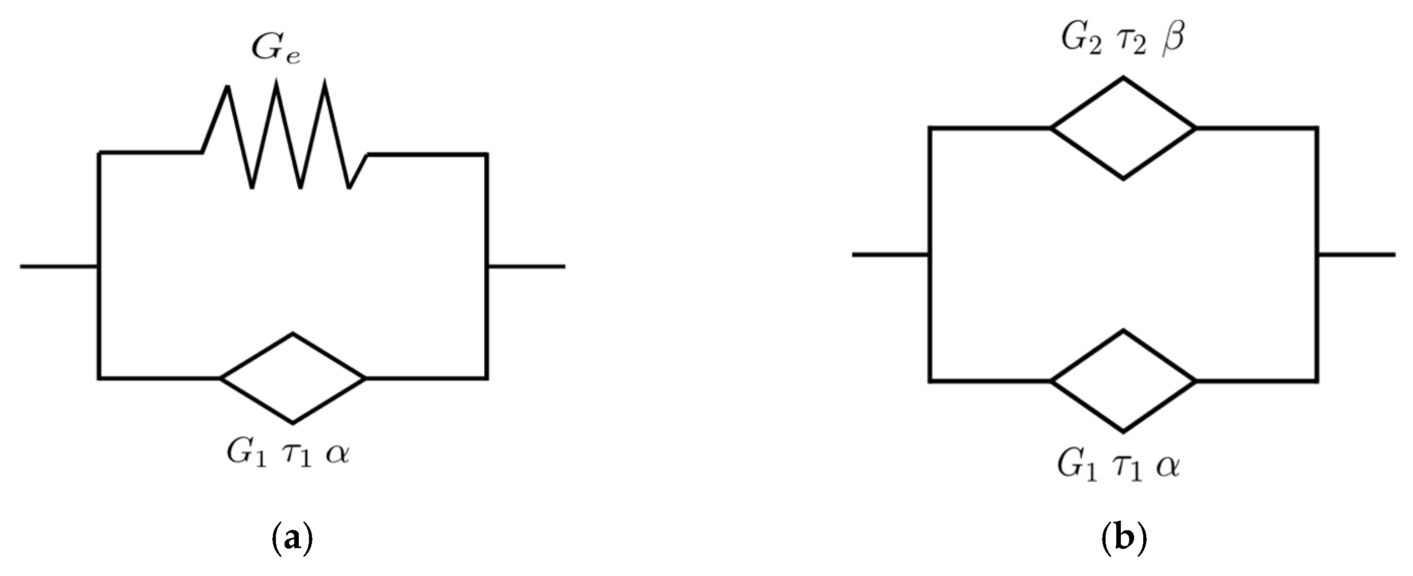
3.4. The Fractional Kelvin Model

The fractional Kelvin model with one spring-pot consists of a spring connected in parallel with one spring-pot. In this model, the dash-pots of the conventional Kelvin model have been replaced by a Scott-Blair element, as shown in Figure 4a.

The constitutive equation is given by:

$$\begin{array}{r}\hfill \mathsf{\sigma }\left(\mathrm{t}\right)={\mathrm{G}}_{\mathrm{e}}{\mathsf{\tau }}^{\mathsf{\alpha }}\frac{{\mathrm{d}}^{\mathsf{\alpha }}\mathsf{\epsilon }\left(\mathrm{t}\right)}{{\mathrm{dt}}^{\mathsf{\alpha }}}+{\mathrm{G}}_{\mathrm{e}}\mathsf{\epsilon }\left(\mathrm{t}\right)\end{array}$$

(34)

where $\mathsf{\alpha }$ is fractional exponents ($0<\mathsf{\alpha }<1$), ${\mathrm{G}}_{\mathrm{e}}$ is the elastic modulus, $\mathsf{\tau }$ is the characteristic time, given by the following expression ${\mathsf{\tau }}^{\mathsf{\alpha }}=\raisebox{1ex}{${\mathrm{G}}_1{\mathsf{\tau }}_1$}\!\left/ \!\raisebox{-1ex}{${\mathrm{G}}_{\mathrm{e}}$}\right.$. The complex modulus of the model can be derived applying Equations (14)–(34), obtaining the following:

$${\mathrm{G}}^{\ast }\left(\mathsf{\omega }\right)=\frac{\tilde{\mathsf{\sigma }}\left(\mathsf{\omega }\right)}{\tilde{\mathsf{\epsilon }}\left(\mathsf{\omega }\right)}={\mathrm{G}}_{\mathrm{e}}(1+(\mathsf{\tau }\mathsf{\omega }\mathrm{i}{)}^{\mathsf{\alpha }})$$

(35)

Separating the real and imaginary parts, we can obtain the storage modulus and loss modulus, respectively:

$$\begin{gathered} {\mathrm{G}}^{\prime }\left(\mathsf{\omega }\right)={\mathrm{G}}_{\mathrm{e}}(1+{(\mathsf{\tau }\mathsf{\omega })}^{\mathsf{\alpha }}\cos (\raisebox{1ex}{$\mathsf{\pi }\mathsf{\alpha }$}\!\left/ \!\raisebox{-1ex}{$2$}\right.)) \\ {\mathrm{G}}^{″}\left(\mathsf{\omega }\right)={\mathrm{G}}_{\mathrm{e}}{(\mathsf{\tau }\mathsf{\omega })}^{\mathsf{\alpha }}\sin \left(\raisebox{1ex}{$\mathsf{\pi }\mathsf{\alpha }$}\!\left/ \!\raisebox{-1ex}{$2$}\right.\right) \end{gathered}$$

(36)

The creep compliance $\mathrm{J}$ is obtained by applying the Laplace transform to Equation (34), obtaining:

$$\mathrm{J}\left(\mathrm{s}\right)=\frac{\mathsf{\epsilon }\left(\mathrm{s}\right)}{\mathrm{s} \mathsf{\sigma }\left(\mathrm{s}\right)}=\frac{1}{{\mathrm{G}}_{\mathrm{e}}\mathrm{s}}\left(1-\frac{{\mathsf{\tau }}^{\mathsf{\alpha }}{\mathrm{s}}^{\mathsf{\alpha }}}{1+{\mathsf{\tau }}^{\mathsf{\alpha }}{\mathrm{s}}^{\mathsf{\alpha }}}\right)$$

(37)

Applying the inverse Laplace transformation, we obtain:

$$\begin{array}{r}\hfill \mathrm{J}\left(\mathrm{t}\right)=\frac{1}{{\mathrm{G}}_{\mathrm{e}}}\left(1-{\mathrm{E}}_{\mathsf{\alpha }}\left(-{\left(\frac{\mathrm{t}}{\mathsf{\tau }}\right)}^{\mathsf{\alpha }}\right)\right)\end{array}$$

(38)

where ${\mathrm{E}}_{\mathsf{\alpha }}$ is the Mittag-Leffler function, with $\mathsf{\beta }=1$, given by the expression:

$${\mathrm{E}}_{\mathsf{\alpha },1}(\mathrm{x})={\displaystyle \sum }_{\mathrm{n}=0}^{\infty }\frac{{\mathrm{x}}^{\mathrm{n}}}{\Gamma \left(\mathsf{\alpha }\mathrm{n}+1\right)}$$

(39)

The fractional Kelvin model with two spring-pots consists of two Scott-Blair elements or spring-pots connected in parallel, as shown in Figure 4b. The constitutive equation is given by:

$$\begin{array}{r}\hfill \mathsf{\sigma }\left(\mathrm{t}\right)={\mathrm{G}\mathsf{\tau }}^{\mathsf{\alpha }}\frac{{\mathrm{d}}^{\mathsf{\alpha }}\mathsf{\epsilon }\left(\mathrm{t}\right)}{{\mathrm{dt}}^{\mathsf{\alpha }}}+{\mathrm{G}\mathsf{\tau }}^{\mathsf{\beta }}\frac{{\mathrm{d}}^{\mathsf{\beta }}\mathsf{\epsilon }\left(\mathrm{t}\right)}{{\mathrm{dt}}^{\mathsf{\beta }}}\end{array}$$

(40)

where $\mathrm{G}$ is an elastic modulus in Pa given by the following expression, $\mathrm{G}={\mathrm{G}}_1{\left(\frac{{\mathsf{\tau }}_1}{\mathsf{\tau }}\right)}^{\mathsf{\alpha }}$ and $\mathsf{\tau }$ is the characteristic time of the model in s, defined by the following expression $\mathsf{\tau }={\left(\raisebox{1ex}{${\mathrm{G}}_1{\mathsf{\tau }}_1^{\mathsf{\alpha }}$}\!\left/ \!\raisebox{-1ex}{${\mathrm{G}}_2{\mathsf{\tau }}_2^{\mathsf{\beta }}$}\right.\right)}^{\raisebox{1ex}{$1$}\!\left/ \!\raisebox{-1ex}{$\mathsf{\alpha }-\mathsf{\beta }$}\right.}$. Applying the Fourier transformation to Equation (40), we obtain:

$${\mathrm{G}}^{\ast }\left(\mathsf{\omega }\right)=\frac{\tilde{\mathsf{\sigma }}\left(\mathsf{\omega }\right)}{\tilde{\mathsf{\epsilon }}\left(\mathsf{\omega }\right)}=\mathrm{G}({(\mathsf{\tau }\mathsf{\omega }\mathrm{i})}^{\mathsf{\alpha }}+\mathsf{\tau }\mathsf{\omega }\mathrm{i}{)}^{\mathsf{\beta }}$$

(41)

Separating the real and imaginary parts, we can obtain the storage modulus and loss modulus, respectively:

$$\begin{gathered} {\mathrm{G}}^{\prime }\left(\mathsf{\omega }\right)=\mathrm{G}\left({(\mathsf{\tau }\mathsf{\omega })}^{\mathsf{\alpha }}\cos (\raisebox{1ex}{$\mathsf{\pi }\mathsf{\alpha }$}\!\left/ \!\raisebox{-1ex}{$2$}\right.)+{(\mathsf{\tau }\mathsf{\omega })}^{\mathsf{\beta }}\cos (\raisebox{1ex}{$\mathsf{\pi }\mathsf{\beta }$}\!\left/ \!\raisebox{-1ex}{$2$}\right.)\right) \\ {\mathrm{G}}^{″}\left(\mathsf{\omega }\right)=\mathrm{G}\left({(\mathsf{\tau }\mathsf{\omega })}^{\mathsf{\alpha }}\sin (\raisebox{1ex}{$\mathsf{\pi }\mathsf{\alpha }$}\!\left/ \!\raisebox{-1ex}{$2$}\right.)+{(\mathsf{\tau }\mathsf{\omega })}^{\mathsf{\beta }}\sin (\raisebox{1ex}{$\mathsf{\pi }\mathsf{\beta }$}\!\left/ \!\raisebox{-1ex}{$2$}\right.)\right) \end{gathered}$$

(42)

The creep compliance J is obtained by applying the Laplace transformation to Equation (40), obtaining:

$$\mathrm{J}\left(\mathrm{s}\right)=\frac{\mathsf{\epsilon }\left(\mathrm{s}\right)}{\mathrm{s} \mathsf{\sigma }\left(\mathrm{s}\right)}=\frac{1}{\mathrm{G}}\left(\frac{{\mathsf{\tau }}^{-\mathsf{\alpha }}{\mathrm{s}}^{-\mathsf{\beta }-1}}{{\mathsf{\tau }}^{\mathsf{\beta }-\mathsf{\alpha }}+{\mathrm{s}}^{\mathsf{\alpha }-\mathsf{\beta }}}\right)$$

(43)

Applying the inverse Laplace transformation, we obtain:

$$\begin{array}{r}\hfill \mathrm{J}\left(\mathrm{t}\right)=\frac{1}{\mathrm{G}}{\left(\frac{\mathrm{t}}{\mathsf{\tau }}\right)}^{\mathsf{\alpha }}{\mathrm{E}}_{\mathsf{\alpha }-\mathsf{\beta },1+\mathsf{\alpha }}\left(-{\left(\frac{\mathrm{t}}{\mathsf{\tau }}\right)}^{\mathsf{\alpha }-\mathsf{\beta }}\right)\end{array}$$

(44)

where ${\mathrm{E}}_{\mathsf{\alpha },\mathsf{\beta }}$ is the Mittag-Leffler function of two parameters, given by the expression:

$${\mathrm{E}}_{\mathsf{\alpha },\mathsf{\beta }}(\mathrm{x})={\displaystyle \sum }_{\mathrm{n}=0}^{\infty }\frac{{\mathrm{x}}^{\mathrm{n}}}{\Gamma \left(\mathsf{\alpha }\mathrm{n}+\mathsf{\beta }\right)}$$

(45)

4. Vortex Search Algorithm (VSA)

The VSA algorithm is a recently developed metaheursistic optimization technique that works with continuous nonlinear non-convex optimization problems in a multidimensional space with dimension $\mathrm{d}$ [37]. This optimization approach works with Gaussian distributions and gamma functions to explore and exploit the solution space. The VSA was inspired by the vortex pattern created by the vortical flow of stirred fluids. In the specialized literature, the VSA has been used in multiple optimization problems as follows: optimal power flow studies in power systems [38,39], optimal location and sizing of capacitor banks and distributed generation in electrical distribution grids [40,41], nonlinear non-convex constrained optimization [42,43], and the selection of analog active filter components, among others. The main aspects of the VSA for numerical optimization are presented below [38]:

• Initial Solution: The VSA works with the vector radius (${\overrightarrow{\mathrm{r}}}_{\mathrm{t}}$ where t is the iteration counter) that generates a hyperellipsoid in a d-dimensional space. To center the hyperellipsoid in the solution space, let us define its center as ${\mathsf{\mu }}_0$, where:

  $$\begin{array}{r}\hfill {\mathsf{\mu }}_0=\frac{{\mathrm{x}}_{\max }+{\mathrm{x}}_{\min }}{2}\end{array}$$

  (46)

  and ${\mathrm{x}}_{\min }\in {ℝ}^{\mathrm{d}\times 1}$ and ${\mathrm{x}}_{\max }\in {ℝ}^{\mathrm{d}\times 1}$ are the minimum and maximum bounds of the solution variables x.
• Candidate Solutions: To generate a set of candidate solutions ${\mathrm{C}}_{\mathrm{i}}^{\mathrm{t}}\left(\mathrm{x}\right)={\mathrm{s}}_{\mathrm{i}}^{\mathrm{t}}={\mathrm{x}}_1.{\mathrm{x}}_2,\dots ,{\mathrm{x}}_{\mathrm{d}}$ (where subscript i is associated with the i-th individual in the population) a Gaussian distribution is used as follows:

  $$\begin{array}{r}\hfill \end{array}\begin{array}{r}\hfill {\mathrm{s}}_{\mathrm{i}}^{\mathrm{t}}=\mathrm{p}\left({\mathsf{\zeta }}_{\mathrm{i}}^{\mathrm{t}},{\mathsf{\mu }}_{\mathrm{t}},\mathrm{v}\right)=\left({(2\mathsf{\pi })}^{\mathrm{d}}\left|\mathsf{\nu }\right|\right){\mathrm{e}}^{\left(-\frac{1}{2}\frac{{\left({\mathsf{\zeta }}_{\mathrm{i}}^{\mathrm{t}}-{\mathsf{\mu }}_{\mathrm{t}}\right)}^{\mathrm{T}}\left({\mathsf{\zeta }}_{\mathrm{i}}^{\mathrm{t}}-{\mathsf{\mu }}_{\mathrm{t}}\right)}{\mathsf{\nu }}\right)}\end{array}$$

  (47)

  where ${\mathsf{\zeta }}_{\mathrm{i}}^{\mathrm{t}}\in {ℝ}^{\mathrm{d}\times 1}$ is a vector of random variables, ${\mathsf{\mu }}_{\mathrm{t}}\in {ℝ}^{\mathrm{d}\times 1}$ is a current center of the hyperellipsoid in the iteration t, and $\mathsf{\nu }\in {ℝ}^{\mathrm{d}\times 1}$ is a matrix of covariances. Here, we simplified this matrix with identical variances ${\mathsf{\sigma }}_0$ in diagonal null covariance, as recommended in [37]:

  $$\begin{array}{r}\hfill {\mathsf{\sigma }}_0=\frac{\max \left\{{\mathrm{x}}_{\max }\right\}-\min \left\{{\mathrm{x}}_{\min }\right\}}{2}\end{array}$$

  (48)

  where $\mathsf{\mu }={\mathsf{\sigma }}_0{\mathrm{I}}_{\mathrm{d}\times \mathrm{d}}$, with $\mathrm{I}$ being an identity matrix with appropriate dimensions. Note that for initializing the radius vector (${\mathrm{r}}_{\mathrm{t}}$ with $\mathrm{t}=0$), the VSA approach recommends assigning it as ${\mathsf{\sigma }}_0$. Note that the vector radius is important in the VSA algorithm, since it governs the random vector of variables ${\mathsf{\zeta }}_{\mathrm{i}}^{\mathrm{t}}$ as ${\mathsf{\zeta }}_{\mathrm{i}}^{\mathrm{t}} \mathrm{rand} \left(\mathrm{d}\right)$, where $\mathrm{rand} \left(\mathrm{d}\right)$ generates a vector of random variables between $0$ and $1$ with dimension $\mathrm{d}$.
• Bounding the Candidate Solutions: Note that a Gaussian distribution can generate a set of solutions ${\mathrm{s}}_{\mathrm{i}}^{\mathrm{t}}$ outside of the solution’s space bounds, which implies that a bounding procedure is always required, as presented below:

  $${\mathrm{s}}_{\mathrm{i}}^{\mathrm{t}}=\{\begin{array}{c}{\mathrm{s}}_{\mathrm{i}}^{\mathrm{t}}{\mathrm{x}}_{\min }\le x\le {\mathrm{x}}_{\max }\\ {\mathrm{x}}_{\min }+\left({\mathrm{x}}_{\max }-{\mathrm{x}}_{\min }\right)\mathrm{rand}\end{array}\begin{array}{cc}& \\ & \mathrm{otherwhise}\end{array}$$

  (49)

  where $\mathrm{rand}$ is a random number between 0 and 1.
• Selection of the new center: To advance through the solution space, it is necessary to select the new center of the hyperellipsoid as a function of the best solution attained in the population, i.e., ${\mathsf{\mu }}_{\mathrm{t}+1}$ must be selected as the individual in ${\mathrm{C}}_{\mathrm{i}}^{\mathrm{t}}\left(\mathrm{x}\right),$ such that it produces the minimum (maximum) solution of the current population, which implies that ${\mathsf{\mu }}_{\mathrm{t}+1}$ = ${\mathrm{s}}_{\mathrm{i},\mathrm{best}}^{\mathrm{t}}$. Observe that the selection of the new center implies that all individuals in the current population have been evaluated in the objective function or in its equivalent [44] to determine the direction of exploration and exploitation of the solution space.
• The Radius Step-Down Process: To decrease the radius of the hyperellipsoid centered at ${\mathsf{\mu }}_{\mathrm{t}+1},$ use the incomplete inverse gamma function [42]; notwithstanding, here we propose an alternative decreasing method using an exponential function as follows [39]:

  $${\mathrm{r}}_{\mathrm{t}+1}={\mathsf{\sigma }}_0\left(1-\frac{\mathrm{t}}{{\mathrm{t}}_{\max }}\right){\mathrm{e}}^{\left(\mathrm{a}\frac{\mathrm{t}}{{\mathrm{t}}_{\max }}\right)}$$

  (50)

  where a is a constant parameter that governs the reduction speed of the radius of the hyperellipsoid that represents the solution space;
• Stopping criteria: The VSA algorithm stops its search process in the solution space when each of the following conditions is reached:
  • If all the iterations have been made, i.e., $\mathrm{t}=$ ${\mathrm{t}}_{\max }$;
  • If during k consecutive iterations the best fitness function has not been modified, with kmax being the maximum consecutive iterations without improvement, i.e., $\mathrm{k}={\mathrm{k}}_{\max }$.

The Vortex Search Algorithm (VSA) was implemented in MATLAB 2019a software. In the parameterization of the VSA a population size of 1000 was considered for the classic and fractional models and several iterations of 500 and 2000 were considered for the classic and fractional models, respectively.

5. Optimization Problem

The parameters of the storage modulus, loss modulus and creep compliance calculated from classical and fractional Maxwell and Kelvin models are estimated using the Vortex Search Algorithm (VSA), based on the minimization of the mean square error between the predicted values (${\mathrm{G}}^{\prime }({\mathsf{\omega }}_{\mathrm{j}}),{\mathrm{G}}^{″}({\mathsf{\omega }}_{\mathrm{j}}),\mathrm{J}\left({\mathrm{t}}_{\mathrm{j}}\right)$) and the measured data (${\mathrm{G}}_{\mathrm{j}}^{\prime },{\mathrm{G}}_{\mathrm{j}}^{″},{\mathrm{J}}_{\mathrm{j}}$). The objective minimization function is given by:

$$\begin{array}{cc}{\mathrm{F}}_{\min } =& {\displaystyle \sum _{\mathrm{j}=1}^{\mathrm{M}}}\left({\left(\frac{{\mathrm{G}}^{\prime }\left({\mathsf{\omega }}_{\mathrm{j}}\right)}{{\mathrm{G}}_{\mathrm{j}}^{\prime }}-1\right)}^2+{\left(\frac{{\mathrm{G}}^{″}\left({\mathsf{\omega }}_{\mathrm{j}}\right)}{{\mathrm{G}}_{\mathrm{j}}^{″}}-1\right)}^2+{\left(\frac{\mathrm{J}\left({\mathrm{t}}_{\mathrm{j}}\right)}{{\mathrm{J}}_{\mathrm{j}}}-1\right)}^2\right)\\ \mathrm{subject} \mathrm{to}& 0<\mathsf{\beta }<\mathsf{\alpha }<1\end{array}$$

(51)

6. Results and Discussion

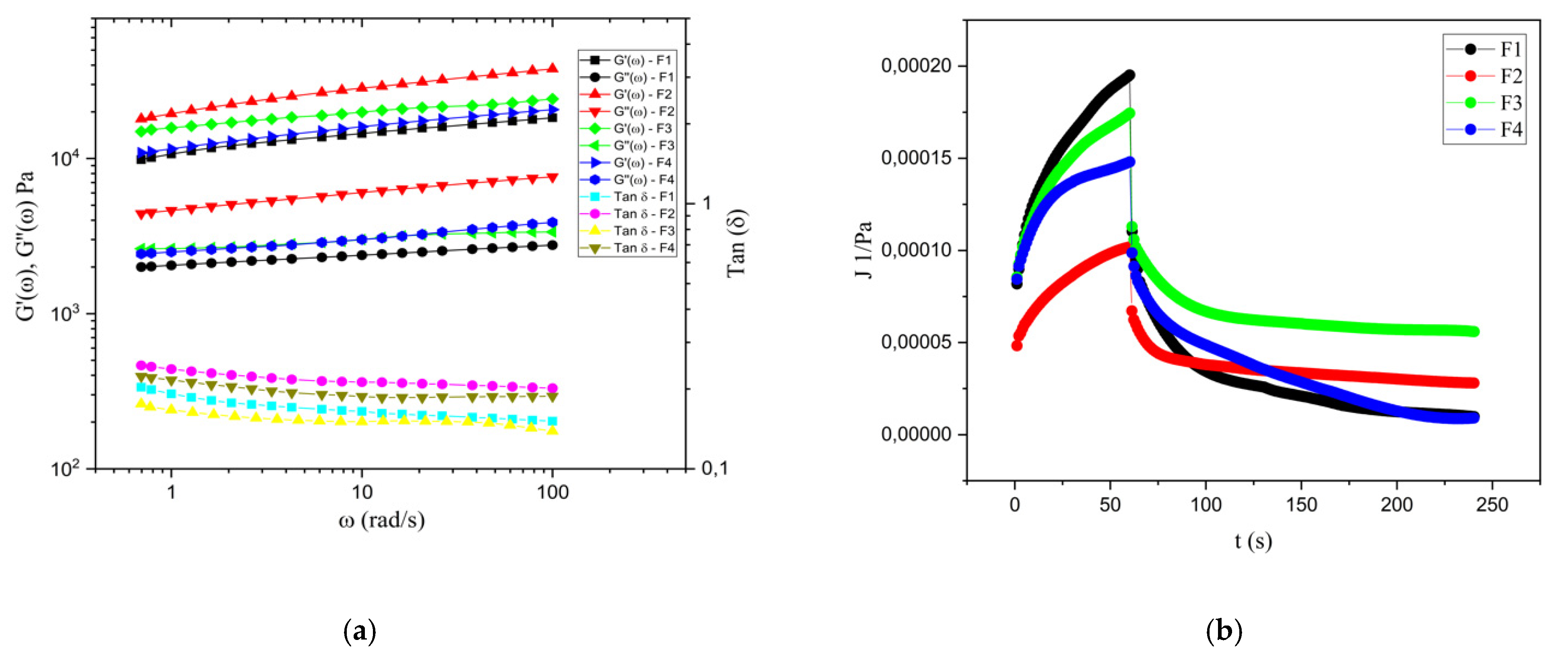
6.1. Viscoelastic Behavior

The storage modulus (${\mathrm{G}}^{\prime }$) and the loss modulus (${\mathrm{G}}^{″}$) characterize the system in the study of rheological dynamics. ${\mathrm{G}}^{\prime }$ is a measure of the energy temporarily stored in a material and ${\mathrm{G}}^{″}$ is a measure of the energy used to activate a flow, energy that is dissipated and transformed into heat [45]. Figure 5a shows the variation of the storage modulus (${\mathrm{G}}^{\prime }$), loss modulus (${\mathrm{G}}^{″}$), and tan $\mathsf{\delta }$ in relation to the angular frequency for formulation sample studies. It can be seen that the elastic behavior for F1, F2, F3, and F4 samples were greater than the viscous behavior (${\mathrm{G}}^{\prime }>{\mathrm{G}}^{″}$) and no crossing points were observed in the angular frequency interval in the study, indicating typical solid viscoelasticity, which is consistent with that reported by González Cuello et al. [46], where it was found that biofilms based on binary mixtures of gellan gum and concentrated whey protein had a viscoelastic solid behavior. The behavior of the modulus ${\mathrm{G}}^{\prime }$ for F1, F2, F3, and F4 is observed to increase and decrease by about the concentration of potassium and calcium ions, respectively, keeping constant the concentrations of carrageenan, gellan gum, and guar gum. A comparison of the values of ${\mathrm{G}}^{\prime }$ of F4 and F3 with F2 and F1, respectively, shows that F2 and F4 show higher ${\mathrm{G}}^{\prime }$. This can be explained because F2 and F4 have a higher concentration of potassium ions in carrageenan than F3 and F1, respectively, which is related to gel formation with greater cross-link formation [13,47,48]; that is, by decreasing the concentration of Carrageenan and potassium ions, the ${\mathrm{G}}^{\prime }$ decreases as well. The presence of calcium ions exerts an influence on the formation of cross-links in gellan gum [49,50,51], observing that, when comparing F2 and F4 with F3 and F1, respectively, when their concentration increases, the values of ${\mathrm{G}}^{\prime }$ decrease, independent of gellan concentration. This may be because the concentrations used were above the optimal gelation value [50]. Studies developed by MacArtain et al. [50] and Meng et al. [49] concluded that, starting with low concentrations of calcium ions, there is an increase in ${\mathrm{G}}^{\prime },$ but as this concentration increases and goes beyond the optimal value, the ${\mathrm{G}}^{\prime }$ values tend to decrease, due to the excess of calcium ions. The third parameter that described the viscoelastic behavior of a material is tan $\mathsf{\delta }$, which is also a function of frequency. Tan $\mathsf{\delta }$ indicates the relationship between the amounts of dissipated and stored energy, i.e., the quantitative relationship between the viscous and the elastic components of a system; then, values of $\tan \mathsf{\delta }>1$ represent a dominant viscous behavior (liquid-like behavior), whereas values of $\tan \mathsf{\delta }<1$ indicate a predominant elastic behavior (solid-like behavior) [52]. The values of $\tan \mathsf{\delta }$ for F1, F2, F3, and F4 are in the range 0.1 to 0.25, indicating that the films under study have an elastic rather than viscous behavior ($\tan \mathsf{\delta }<1$). Figure 5b shows the creep and recovery curves for the hydrocolloid films in the study. It can be seen that all of the samples showed a recovery when the applied stress was removed, showing a solid viscoelastic behavior consistent with the results obtained with the storage and loss modulus. Gonzalez Cuello et al. [46] reported similar results for films prepared from binary mixtures.

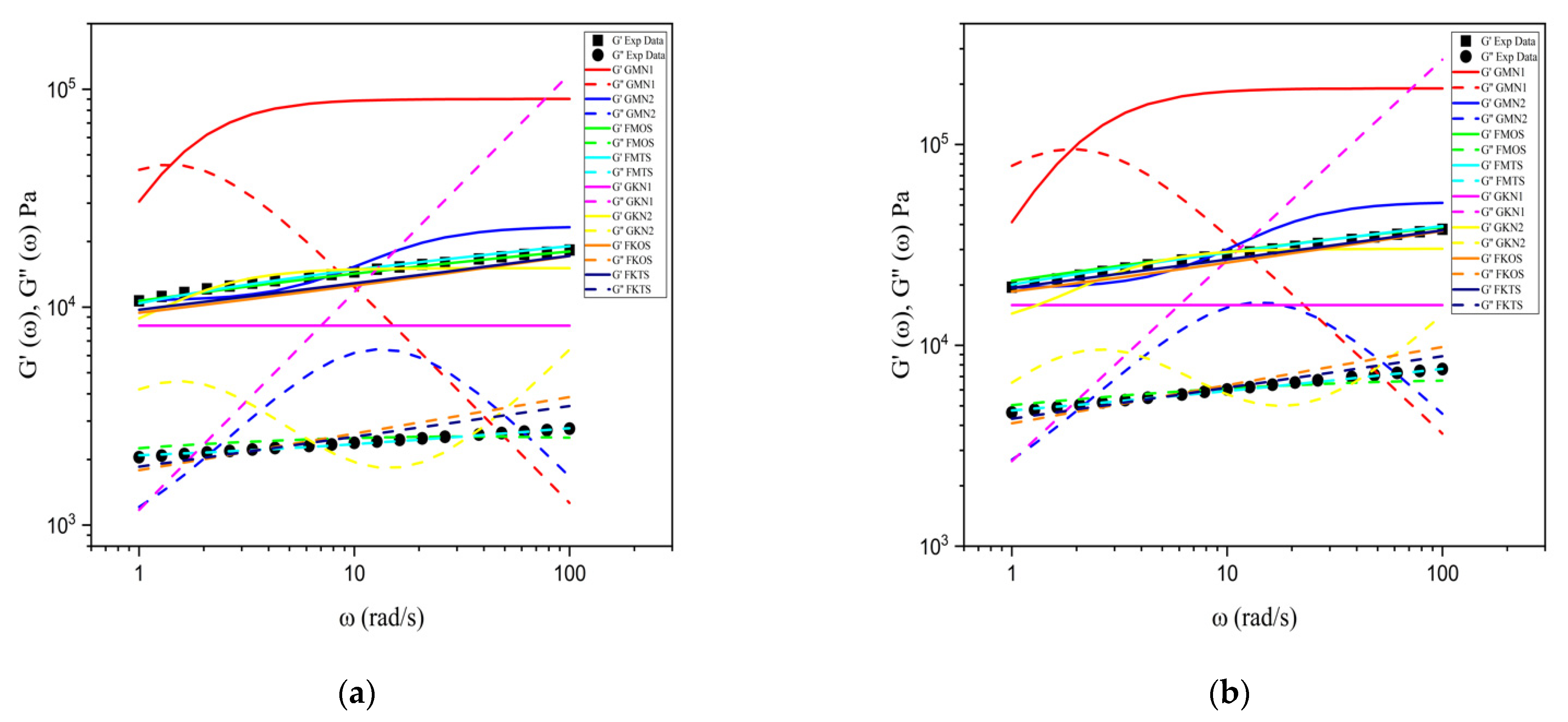
6.2. Validation of the Viscoelastic Rheological Model

Figure 6 and Figure 7 show the fit of the experimental data of the dynamic rheological and creep behaviors with the Maxwell and Kelvin generalized models for N = 1 and N = 2 and with the fractional Maxwell and Kelvin models. From the models evaluated to describe the viscoelastic behavior of hydrocolloid-based films, we can observe that Maxwell’s fractional model with two spring-pots shows a good fit for the experimental data of ${\mathrm{G}}^{\prime }$, ${\mathrm{G}}^{″}$, and creep compliance.

Table 2. Optimal values F_min.

Rheological Model	F1	F2	F3	F4
Generalized Maxwell N = 1	52.751	55.906	52.974	57.504
Generalized Maxwell N = 2	4.853	5.044	5.624	5.487
Fractional Maxwell with one spring-pot	0.343	0.222	0.605	0.122
Fractional Maxwell with two spring-pot	0.031	0.033	0.087	0.044
Generalized Kelvin N = 1	32.151	34.272	46.119	26.171
Generalized Kelvin N = 2	4.390	3.882	3.856	2.751
Fractional Kelvin with one spring-pot	1.623	0.828	3.288	0.371
Fractional Kelvin with two spring-pot	1.117	0.413	2.240	0.141

shows the optimal value of the objective function (Equation (51) for the models under study. For the generalized Maxwell and Kelvin models, the value of ${\mathrm{F}}_{\min }$ decreases as the value of N increases, and in the same way for fractional models, this can be explained by the increase in the number of parameters of the models. Comparing the results of ${\mathrm{F}}_{\min }$ of the classical models with the fractional ones according to the number of parameters, we can observe that the generalized Maxwell and Kelvin models for N = 1 and N = 2 show high values compared to the fractional models. Between the Maxwell and Kelvin models with one and two spring-pots, Maxwell’s fractional model with two spring-pots was the one that presents the lowest values of ${\mathrm{F}}_{\min }$, indicating that this model is the one that shows the best fit of the experimental data of ${\mathrm{G}}^{\prime }$ and ${\mathrm{G}}^{″}$.

Table 3. R² for creep compliance models.

Rheological Model	F1	F2	F3	F4
Generalized Maxwell N = 1	/	/	/	/
Generalized Maxwell N = 2	0.79	0.83	0.15	0.58
Fractional Maxwell with one spring-pot	0.90	0.95	0.98	0.98
Fractional Maxwell with two spring-pot	0.99	0.99	0.98	0.98
Generalized Kelvin N = 1	/	/	/	/
Generalized Kelvin N = 2	0.21	0.12	0.71	0.07
Fractional Kelvin with one spring-pot	0.65	0.76	0.60	0.88
Fractional Kelvin with two spring-pot	0.72	0.85	0.71	0.95

shows the values of ${\mathrm{R}}^2$ for the adjustment of the experimental data of creep compliance and the rheological models under study. For the Maxwell and Kelvin generalized models with N = 1, values of ${\mathrm{R}}^2<0$ were obtained, indicating no adjustments to the experimental data. For F2, the generalized Maxwell model with N = 2 shows a value of ${\mathrm{R}}^2=0.15$, indicating a poor fit to the experimental data.

The generalized Kelvin model with N = 2 presented ${\mathrm{R}}^2$ values between 0.07 and 0.71, which indicates that the model does not show a good fit for all the formulations under study. Maxwell’s fractional model with two spring-pots for all the formulations under study presented values of ${\mathrm{R}}^2>0.98$, which indicates a good fit of the experimental data of creep compliance.

These results show that the fractional models fit the experimental data of ${\mathrm{G}}^{\prime }$, ${\mathrm{G}}^{″}$, and creep compliance J better than the classical models, using a lesser or equal number of parameters. Bonfanti et al. [53] reported similar results in their review, where they concluded that fractional viscoelastic models can accurately capture the rheological responses of a wide range of materials using fewer parameters than traditional viscoelastic models.

Table 4. Estimate of the Maxwell fractional parameter with the two spring-pot model.

Sample Code	$\mathbf{G} \left(\mathbf{P}\mathbf{a}\right)$	$\mathsf{\tau } \left(\mathbf{s}\right)$	$\mathsf{\alpha }$	$\mathsf{\beta }$
F1	8487.75	139.65	0.57	0.09
F2	11171.42	557.46	0.56	0.12
F3	13335.38	41.03	0.42	0.08
F4	5145.16	1537.85	0.89	0.12

shows the parameters fitted to the Maxwell model with two spring-pots. It is observed that for a fixed composition of 0.25 and 1.35 of gellan gum and carrageenan, the G modulus tends to increase its magnitude when the concentrations of potassium citrate and calcium chloride increase and decrease respectively, while at fixed compositions of 0.4 and 1.2, the G modulus tends to decrease in magnitude when the concentrations of potassium citrate and calcium chloride increase and decrease, respectively. It is also observed that if the concentration of gellan gum and carrageenan is increased and decreased for the fixed concentrations of 0.2 and 0.4, the magnitude of the G modulus tends to increase, and for concentrations of 0.4 and 0.2, when increasing and decreasing the concentration of gellan gum and carrageenan, respectively, the magnitude of the G modulus tends to decrease. The above shows that the G modulus is influenced by the concentrations of the gums used and the concentrations of potassium citrate and calcium chloride.

7. Conclusions

The hydrocolloid-based films obtained in this study presented viscoelastic-type rheological behavior. The results of the dynamic tests showed that the elastic component of the hydrocolloid-based films was greater than the viscous component (${\mathrm{G}}^{\prime }>$ ${\mathrm{G}}^{″}$). The hydrocolloid-based films showed recovery when the applied stress was suspended, showing a viscoelastic solid behavior. The presence of calcium and potassium ions showed an influence on the viscoelastic behavior of hydrocolloid-based films. It was observed that the elastic modulus $\mathrm{G}$ increases and decreases with increasing concentrations of calcium and potassium ions, respectively. The rheological model parameters for dynamic and creep behavior were adjusted using the Vortex Search Algorithm (VSA). The results of the objective function ${\mathrm{F}}_{\min }$ and ${\mathrm{R}}^2$ for the films obtained with formulations F1, F2, F3, and F4 show that the Maxwell fractional model with two spring-pots optimally adjusts the dynamic and creep rheological behaviors.

The above shows the importance of estimating parameters that allow for a description of the dynamic rheological and creep behaviors of hydrocolloid-based films for future applications in the design of active films, since they allow for an understanding of their behavior, from a rheological point of view, which can contribute to the design and improvement of products, such as food coatings, food packaging or other applications containing biopolymers. Therefore, this work could allow the design of biodegradable packaging from new hydrocolloid formulations.

References

1. Hasan, M.; Rusman, R.; Khaldun, I.; Ardana, L.; Mudatsir, M.; Fansuri, H. Active Edible Sugar Palm Starch-Chitosan Films Carrying Extra Virgin Olive Oil: Barrier, Thermo-Mechanical, Antioxidant, and Antimicrobial Properties. Int. J. Biol. Macromol. 2020, 163, 766–775. [Google Scholar] [CrossRef] [PubMed]
2. León, P.G.; Chillo, S.; Conte, A.; Gerschenson, L.N.; Del Nobile, M.A.; Rojas, A.M. Rheological Characterization of Deacylated/Acylated Gellan Films Carrying l-(+)-Ascorbic Acid. Food Hydrocoll. 2009, 23, 1660–1669. [Google Scholar] [CrossRef]
3. Skendi, A.; Biliaderis, C.G.; Lazaridou, A.; Izydorczyk, M.S. Structure and Rheological Properties of Water Soluble β-Glucans from Oat Cultivars of Avena Sativa and Avena Bysantina. J. Cereal Sci. 2003, 38, 15–31. [Google Scholar] [CrossRef]
4. Mali, S.; Grossmann, M.V.E.; García, M.A.; Martino, M.N.; Zaritzky, N.E. Mechanical and Thermal Properties of Yam Starch Films. Food Hydrocoll. 2005, 19, 157–164. [Google Scholar] [CrossRef]
5. Suhag, R.; Kumar, N.; Petkoska, A.T.; Upadhyay, A. Film Formation and Deposition Methods of Edible Coating on Food Products: A Review. Food Res. Int. 2020, 136, 109582. [Google Scholar] [CrossRef]
6. Coutinho, D.F.; Sant, S.V.; Shin, H.; Oliveira, J.T.; Gomes, M.E.; Neves, N.M.; Khademhosseini, A.; Reis, R.L. Modified Gellan Gum Hydrogels with Tunable Physical and Mechanical Properties. Biomaterials 2010, 31, 7494–7502. [Google Scholar] [CrossRef] [PubMed] [Green Version]
7. Goyal, R.; Tripathi, S.K.; Tyagi, S.; Ram, K.R.; Ansari, K.M.; Shukla, Y.; Chowdhuri, D.K.; Kumar, P.; Gupta, K.C. Gellan Gum Blended PEI Nanocomposites as Gene Delivery Agents: Evidences from in Vitro and in Vivo Studies. Eur. J. Pharm. Biopharm. 2011, 79, 3–14. [Google Scholar] [CrossRef] [PubMed]
8. De Filpo, G.; Palermo, A.M.; Munno, R.; Molinaro, L.; Formoso, P.; Nicoletta, F.P. Gellan Gum/Titanium Dioxide Nanoparticle Hybrid Hydrogels for the Cleaning and Disinfection of Parchment. Int. Biodeterior. Biodegrad. 2015, 103, 51–58. [Google Scholar] [CrossRef]
9. Vilela, J.A.P.; de Assis Perrechil, F.; Picone, C.S.F.; Sato, A.C.K.; da Cunha, R.L. Preparation, Characterization and in Vitro Digestibility of Gellan and Chitosan–Gellan Microgels. Carbohydr. Polym. 2015, 117, 54–62. [Google Scholar] [CrossRef]
10. Rukmanikrishnan, B.; Ismail, F.R.M.; Manoharan, R.K.; Kim, S.S.; Lee, J. Blends of Gellan Gum/Xanthan Gum/Zinc Oxide Based Nanocomposites for Packaging Application: Rheological and Antimicrobial Properties. Int. J. Biol. Macromol. 2020, 148, 1182–1189. [Google Scholar] [CrossRef]
11. Fouda, M.M.G.; El-Aassar, M.R.; El Fawal, G.F.; Hafez, E.E.; Masry, S.H.D.; Abdel-Megeed, A. K-Carrageenan/Poly Vinyl Pyrollidone/Polyethylene Glycol/Silver Nanoparticles Film for Biomedical Application. Int. J. Biol. Macromol. 2015, 74, 179–184. [Google Scholar] [CrossRef] [PubMed]
12. Ganesan, A.R.; Munisamy, S.; Bhat, R. Effect of Potassium Hydroxide on Rheological and Thermo-Mechanical Properties of Semi-Refined Carrageenan (SRC) Films. Food Biosci. 2018, 26, 104–112. [Google Scholar] [CrossRef]
13. Bui, V.T.N.T.; Nguyen, B.T.; Nicolai, T.; Renou, F. Mixed Iota and Kappa Carrageenan Gels in the Presence of Both Calcium and Potassium Ions. Carbohydr. Polym. 2019, 223, 115107. [Google Scholar] [CrossRef]
14. Phan The, D.; Debeaufort, F.; Voilley, A.; Luu, D. Biopolymer Interactions Affect the Functional Properties of Edible Films Based on Agar, Cassava Starch and Arabinoxylan Blends. J. Food Eng. 2009, 90, 548–558. [Google Scholar] [CrossRef]
15. Silva-Weiss, A.; Bifani, V.; Ihl, M.; Sobral, P.J.A.; Gómez-Guillén, M.C. Polyphenol-Rich Extract from Murta Leaves on Rheological Properties of Film-Forming Solutions Based on Different Hydrocolloid Blends. J. Food Eng. 2014, 140, 28–38. [Google Scholar] [CrossRef] [Green Version]
16. Dogan, H.; Kokini, J.L. Rheological Properties of Foods. In Handbook Food Engineering, 2nd ed.; Heldman, D., Lund, D., Eds.; CRC Press: Boca Raton, FL, USA, 2007; pp. 1–124. [Google Scholar]
17. Del Nobile, M.A.; Chillo, S.; Mentana, A.; Baiano, A. Use of the Generalized Maxwell Model for Describing the Stress Relaxation Behavior of Solid-like Foods. J. Food Eng. 2007, 78, 978–983. [Google Scholar] [CrossRef]
18. Lu, H.; Ma, D.; Wang, J.; Yu, J. Research on Mechanical Behavior of Viscoelastic Food Material in the Mode of Compressed Chewing. Math. Probl. Eng. 2015, 2015, 581424. [Google Scholar] [CrossRef] [Green Version]
19. Mahiuddin, M.; Khan, M.I.H.; Pham, N.D.; Karim, M.A. Development of Fractional Viscoelastic Model for Characterizing Viscoelastic Properties of Food Material during Drying. Food Biosci. 2018, 23, 45–53. [Google Scholar] [CrossRef] [Green Version]
20. Mahiuddin, M.; Godhani, D.; Feng, L.; Liu, F.; Langrish, T.; Karim, M.A. Application of Caputo Fractional Rheological Model to Determine the Viscoelastic and Mechanical Properties of Fruit and Vegetables. Postharvest Biol. Technol. 2020, 163, 111147. [Google Scholar] [CrossRef]
21. Di Paola, M.; Pirrotta, A.; Valenza, A. Visco-Elastic Behavior through Fractional Calculus: An Easier Method for Best Fitting Experimental Results. Mech. Mater. 2011, 43, 799–806. [Google Scholar] [CrossRef] [Green Version]
22. Drăgănescu, G.E. Application of a Variational Iteration Method to Linear and Nonlinear Viscoelastic Models with Fractional Derivatives. J. Math. Phys. 2006, 47, 082902. [Google Scholar] [CrossRef]
23. Kontou, E.; Katsourinis, S. Application of a Fractional Model for Simulation of the Viscoelastic Functions of Polymers. J. Appl. Polym. Sci. 2016, 133, 43505. [Google Scholar] [CrossRef]
24. Xu, Z.; Chen, W. A Fractional-Order Model on New Experiments of Linear Viscoelastic Creep of Hami Melon. Comput. Math. Appl. 2013, 66, 677–681. [Google Scholar] [CrossRef]
25. Jaishankar, A.; McKinley, G.H. A Fractional K-BKZ Constitutive Formulation for Describing the Nonlinear Rheology of Multiscale Complex Fluids. J. Rheol. 2014, 58, 1751–1788. [Google Scholar] [CrossRef] [Green Version]
26. Ma, L.; Barbosa-Cánovas, G.V. Simulating viscoelastic properties of selected food gums and gum mixtures using a fractional derivative model. J. Texture Stud. 1996, 27, 307–325. [Google Scholar] [CrossRef]
27. Arikoglu, A. A New Fractional Derivative Model for Linearly Viscoelastic Materials and Parameter Identification via Genetic Algorithms. Rheol. Acta 2014, 53, 219–233. [Google Scholar] [CrossRef]
28. Ciniello, A.P.D.; Bavastri, C.A.; Pereira, J.T. Identifying Mechanical Properties of Viscoelastic Materials in Time Domain Using the Fractional Zener Model. Lat. Am. J. Solids Struct. 2017, 14, 131–152. [Google Scholar] [CrossRef] [Green Version]
29. Amabili, M.; Balasubramanian, P.; Breslavsky, I. Anisotropic Fractional Viscoelastic Constitutive Models for Human Descending Thoracic Aortas. J. Mech. Behav. Biomed. Mater. 2019, 99, 186–197. [Google Scholar] [CrossRef] [PubMed]
30. Palacio-Torralba, J.; Hammer, S.; Good, D.W.; Alan McNeill, S.; Stewart, G.D.; Reuben, R.L.; Chen, Y. Quantitative Diagnostics of Soft Tissue through Viscoelastic Characterization Using Time-Based Instrumented Palpation. J. Mech. Behav. Biomed. Mater. 2015, 41, 149–160. [Google Scholar] [CrossRef] [Green Version]
31. Müller, S.; Kästner, M.; Brummund, J.; Ulbricht, V. On the Numerical Handling of Fractional Viscoelastic Material Models in a FE Analysis. Comput. Mech. 2013, 51, 999–1012. [Google Scholar] [CrossRef]
32. Palomares-Ruiz, J.E.; Rodriguez-Madrigal, M.; Lugo, J.G.C.; Rodriguez-Soto, A.A. Fractional Viscoelastic Models Applied to Biomechanical Constitutive Equations. Rev. Mex. Fis. 2015, 61, 261–267. [Google Scholar]
33. Yin, B.; Hu, X.; Song, K. Evaluation of Classic and Fractional Models as Constitutive Relations for Carbon Black–Filled Rubber. J. Elastomers Plast. 2018, 50, 463–477. [Google Scholar] [CrossRef]
34. Zhang, H.; Li, S.; Zhang, Z.; Luo, H.; Wang, Y. A Five-Parameter Fractional Derivative Temperature Spectrum Model for Polymeric Damping Materials. Polym. Test. 2020, 89, 106654. [Google Scholar] [CrossRef]
35. Faber, T.J.; Jaishankar, A.; McKinley, G.H. Describing the Firmness, Springiness and Rubberiness of Food Gels Using Fractional Calculus. Part I: Theoretical Framework. Food Hydrocoll. 2017, 62, 311–324. [Google Scholar] [CrossRef]
36. Schiessel, H.; Metzler, R.; Blumen, A.; Nonnenmacher, T.F. Generalized Viscoelastic Models: Their Fractional Equations with Solutions. J. Phys. A Math. Gen. 1995, 28, 6567–6584. [Google Scholar] [CrossRef]
37. Doğan, B.; Ölmez, T. A New Metaheuristic for Numerical Function Optimization: Vortex Search Algorithm. Inf. Sci. 2015, 293, 125–145. [Google Scholar] [CrossRef]
38. Figueroa-García, J.C.; Duarte-González, M.; Jaramillo-Isaza, S.; Orjuela-Cañon, A.D.; Díaz-Gutierrez, Y. (Eds.) Applied Computer Sciences in Engineering. In Proceedings of the 6th Workshop on Engineering Applications, WEA 2019, Santa Marta, Colombia, 16–18 October 2019; Communications in Computer and Information Science. Springer International Publishing: Cham, Switzerland, 2019; Volume 1052, ISBN 978-3-030-31018-9. [Google Scholar]
39. Montoya, O.D.; Gil-Gonzalez, W.; Grisales-Norena, L.F. Vortex Search Algorithm for Optimal Power Flow Analysis in DC Resistive Networks With CPLs. IEEE Trans. Circuits Syst. II 2020, 67, 1439–1443. [Google Scholar] [CrossRef]
40. Montoya, O.D.; Gil-González, W.; Orozco-Henao, C. Vortex Search and Chu-Beasley Genetic Algorithms for Optimal Location and Sizing of Distributed Generators in Distribution Networks: A Novel Hybrid Approach. Eng. Sci. Technol. Int. J. 2020, 23, 1351–1363. [Google Scholar] [CrossRef]
41. Gil-González, W.; Montoya, O.D.; Rajagopalan, A.; Grisales-Noreña, L.F.; Hernández, J.C. Optimal Selection and Location of Fixed-Step Capacitor Banks in Distribution Networks Using a Discrete Version of the Vortex Search Algorithm. Energies 2020, 13, 4914. [Google Scholar] [CrossRef]
42. Dogan, B. A Modified Vortex Search Algorithm for Numerical Function Optimization. IJAIA 2016, 7, 37–54. [Google Scholar] [CrossRef]
43. Li, P.; Zhao, Y. A Quantum-Inspired Vortex Search Algorithm with Application to Function Optimization. Nat. Comput. 2019, 18, 647–674. [Google Scholar] [CrossRef]
44. Doğan, B.; Ölmez, T. Vortex Search Algorithm for the Analog Active Filter Component Selection Problem. AEU Int. J. Electron. Commun. 2015, 69, 1243–1253. [Google Scholar] [CrossRef]
45. Lee, K.Y.; Kim, Y.-R.; Park, K.H.; Lee, H.G. Rheological and Gelation Properties of Rice Starch Modified with 4-α-Glucanotransferase. Int. J. Biol. Macromol. 2008, 42, 298–304. [Google Scholar] [CrossRef] [PubMed]
46. González Cuello, R.E.; Urbina, N.A.; Morón Alcázar, L. Caracterización Viscoelástica de Biopelículas Obtenidas a Base de Mezclas Binarias. Inf. Tecnológica 2015, 26, 71–76. [Google Scholar] [CrossRef]
47. Núñez-Santiago, M.C.; Tecante, A.; Garnier, C.; Doublier, J.L. Rheology and Microstructure of κ-Carrageenan under Different Conformations Induced by Several Concentrations of Potassium Ion. Food Hydrocoll. 2011, 25, 32–41. [Google Scholar] [CrossRef]
48. Thrimawithana, T.R.; Young, S.; Dunstan, D.E.; Alany, R.G. Texture and Rheological Characterization of Kappa and Iota Carrageenan in the Presence of Counter Ions. Carbohydr. Polym. 2010, 82, 69–77. [Google Scholar] [CrossRef]
49. Meng, Y.C.; Hong, L.B.; Jin, J.Q. A Study on the Gelation Properties and Rheological Behavior of Gellan Gum. AMM 2013, 284–287, 20–24. [Google Scholar] [CrossRef]
50. MacArtain, P.; Jacquier, J.C.; Dawson, K.A. Physical Characteristics of Calcium Induced κ-Carrageenan Networks. Carbohydr. Polym. 2003, 53, 395–400. [Google Scholar] [CrossRef]
51. Watase, M.; Nishinari, K. Effect of Potassium Ions on the Rheological and Thermal Properties of Gellan Gum Gels. Food Hydrocoll. 1993, 7, 449–456. [Google Scholar] [CrossRef]
52. De Vries, A.; Wesseling, A.; van der Linden, E.; Scholten, E. Protein Oleogels from Heat-Set Whey Protein Aggregates. J. Colloid Interface Sci. 2017, 486, 75–83. [Google Scholar] [CrossRef]
53. Bonfanti, A.; Kaplan, J.L.; Charras, G.; Kabla, A. Fractional Viscoelastic Models for Power-Law Materials. Soft Matter 2020, 16, 6002–6020. [Google Scholar] [CrossRef] [PubMed]
Figure 1. Generalized Maxwell model.
Fluids 06 00418 g001
Figure 2. Maxwell fractional model with (a) one spring-pot; (b) two spring-pots.
Fluids 06 00418 g002
Figure 3. The generalized Kelvin models.
Fluids 06 00418 g003
Figure 4. Kelvin fractional model with (a) one spring-pot; (b) two spring-pots.
Fluids 06 00418 g004
Figure 5. Viscoelastic properties of hydrocolloids films: (a) behavior of dynamic module ( G , G ) and tangent of the phase angle (Tan δ ) in relation to frequency; (b) creep and recovery curves of hydrocolloid films.
Fluids 06 00418 g005
Figure 6. Experimental values of the storage and the loss modulus and generalized Maxwell and Kelvin models (N = 1 and N = 2), fractional Maxwell models with one and two spring-pots, and fractional Kelvin models with one and two spring pots: (a) F1; (b) F2; (c) F3; (d) F4. (GMN1: Generalized Maxwell model (N = 1); GMN2: Generalized Maxwell model (N = 2); FMOS: Fractional Maxwell Model with One Spring-pot; FMTS: Fractional Maxwell Model with Two Spring-pots; GKN1: Generalized Kelvin model (N = 1); GKN2: Generalized Kelvin model (N = 2); FKOS: Fractional Kelvin Model with One Spring-pot; FKTS: Fractional Kelvin Model with Two Spring-pots.)
Fluids 06 00418 g006aFluids 06 00418 g006b
Figure 7. The experimental values of creep compliance and generalized Maxwell and Kelvin models (N = 1 and N= 2), fractional Maxwell models with one and two spring-pots, and fractional Kelvin models with one and two spring-pots: (a) F1; (b) F2; (c) F3; (d) F4. (GMN1: Generalized Maxwell model (N = 1); GMN2: Generalized Maxwell model (N = 2); FMOS: Fractional Maxwell Model with One Spring-pot; FMTS: Fractional Maxwell Model with Two Spring-pots; GKN1: Generalized Kelvin model (N = 1); GKN2: Generalized Kelvin model (N = 2); FKOS: Fractional Kelvin Model with One Spring-pot; FKTS: Fractional Kelvin Model with Two Spring-pots).
Fluids 06 00418 g007aFluids 06 00418 g007b