Low-Speed DSMC Simulations of Hotwire Anemometers at High-Altitude Conditions


Smead Aerospace Engineering Sciences, University of Colorado Boulder, Boulder, CO 80303, USA
*
Author to whom correspondence should be addressed.
Fluids 2021, 6(1), 20; https://doi.org/10.3390/fluids6010020
Submission received: 1 December 2020
/
Revised: 24 December 2020
/
Accepted: 28 December 2020
/
Published: 2 January 2021
(This article belongs to the Special Issue Rarefied Gas Dynamics)
Abstract
:Numerical simulations of hotwire anemometers in low-speed, high-altitude conditions have been carried out using the direct simulation Monte Carlo (DSMC) method. Hotwire instruments are commonly used for in-situ turbulence measurements because of their ability to obtain high spatial and temporal resolution data. Fast time responses are achieved by the wires having small diameters (1–5 m). Hotwire instruments are currently being used to make in-situ measurements of high-altitude turbulence (20–40 km). At these altitudes, hotwires experience Knudsen number values that lie in the transition-regime between slip-flow and free-molecular flow. This article expands the current knowledge of hotwire anemometers by investigating their behavior in the transition-regime. Challenges involved with simulating hotwires at high Knudsen number and low Reynolds number conditions are discussed. The ability of the DSMC method to simulate hotwires from the free-molecular to slip-flow regimes is demonstrated. Dependence of heat transfer on surface accommodation coefficient is explored and discussed. Simulation results of Nusselt number dependence on Reynolds number show good agreement with experimental data. Magnitude discrepancies are attributed to differences between simulation and experimental conditions, while discrepancies in trend are attributed to finite simulation domain size.
Keywords:
DSMC; rarefied; transition-regime; hotwire; Nusselt number; calibration; low-speed; Reynolds number1. Introduction
Recent demand for hypersonic vehicles requires an increased understanding of turbulence in the stratosphere, the region of the atmosphere in which these vehicles will likely cruise. The Hypersonic Flight in the Turbulent Stratosphere (HYFLITS) research campaign, supported by the Air Force Office of Scientific Research (AFOSR) Multidisciplinary University Research Initiative (MURI), is making in-situ measurements of stratospheric turbulence with balloon-borne hotwire anemometers. Hotwires have long been used to measure turbulent fluctuations of velocity. Calibration of these anemometers is a crucial step in this research effort. The balloon-borne instruments will experience mean flow rates between 1 and 10 m/s. Corresponding hotwire Reynolds number (Re) values at the altitudes of interest have a wide range, . Low air density in the stratosphere results in fine-wire Knudsen number values (, where is the mean free path) in the range based on a wire diameter of m. These values correspond to the transition-regime between slip-flow and free-molecular flow. Extensive theoretical and experimental studies have been conducted for hotwires in the continuum (Kn ) and slip-flow ( Kn ) regimes [1,2,3,4,5]. Little work has been published that addresses the behavior of hotwires in the transition-regime ( Kn ) [6,7].
The seminal work for hotwire instruments is that of King [1] who first derived a relationship (known as King’s law) between wire energy transfer and streaming velocity. King’s law can be expressed in non-dimensional form as
Re is the wire Reynolds number given by
where is the fluid density, is the fluid dynamic viscosity, and is the free-stream fluid velocity. Nusselt number, Nu, is the non-dimensional ratio of the convective and conductive energy transfer from the wire and is given by
where k is the thermal conductivity of the fluid and h is the convective heat transfer coefficient,
In Equation (4), Q is the heat transfer from the wire surface to the surrounding fluid, is the wire temperature, is the free-stream gas temperature, and A is the surface area of the wire. In equation [1], the values for , , and n are determined by experimental calibration. The original derivation of King [1] suggested a value of 0.5 for n. This has been shown to be fairly accurate for Re , the value at which vortex-shedding commences [2]. Collis and Williams [2] experimentally investigate hotwires in low Reynolds number flows. They propose a slightly different calibration law that includes an explicit dependence on the film and free-stream temperatures:
Values for , , and n are different depending on whether Re is above or below the value at which vortex shedding occurs. The temperature ratio is included as a way of taking into account the fact that fluid properties are a function of temperature.
An experimental study by Andrews et al. [5] explores the dependence of Nu on Kn. Experimental results are presented for Kn values up to about 0.1. The relationship they propose has the same form as Equation (1) with , , and . The value for Nu given by Equation (1) with the provided constants is referred to as the continuum Nusselt number. This value of Nu differs from the measured value, Nu, because of the thermal slip at the wire surface when wire Kn is in the slip-flow regime. A correction to the continuum Nu to obtain the measured Nusselt number Nu is given as
Equation (6) is derived from kinetic theory and a first-order approximation of the temperature-jump boundary condition. The value for depends on the accommodation coefficient at the surface of the wire. A value of successfully captured the slip affects seen in the experimental data of Andrews et al. [5]. Equation (6) was also presented in Collis and Williams [2], though they did not have enough experimental data to thoroughly expound upon its validity. A similar expression was derived in the extensive theoretical study of Kassoy [4].
Equation (6) is limited by the fact that its derivation depends on a first-order approximation of the thermal slip at the wire surface [8]. This assumption degrades at higher Kn values because property gradients are no longer linear over a distance approximately equal to the mean free path. Second-order slip boundary conditions were derived by Deissler [8]. Although these boundary conditions have not been used to derive solutions for hotwire heat transfer, they show only a slight improvement over first-order boundary conditions in terms of the applicable range of Kn.
An experimental study by Xie et al. [6] presents hotwire heat transfer results in the transition-regime and velocities between 0.5 and 20 m/s (, ). Their results show a clear decrease in Nu with increasing Kn. They present an empirical correlation for Nu as a function of Re and Kn:
Values for the constants in Equation (7) are calculated using a non-linear least-squares fit to the experimental data. No physical justification was given for Equation (7). Data published by Xie et al. [6] and a subsequent study by the same group are the only transition-regime hotwire experimental results that the authors are aware of [7].
Few numerical simulation investigations of fine-wire heat transfer have been conducted [7,9,10,11,12]. Çelenligil [12] uses the direct simulation Monte Carlo (DSMC) method to explore heat transfer to cylinders with Kn = 0.02 and 0.2. Cylinder Re ranged from 0.6 to 24. In Xie et al. [7], slip-flow boundary conditions are derived and implemented into the ANYSYS Fluent finite volume computational fluid dynamics (CFD) solver. The study is limited to low wire temperatures relative to the free-stream ( C) to avoid implementing temperature-dependent fluid properties. At Kn , simulation results show good agreement with selected experimental data from Xie et al. [6] and with several published Nu correlations including Collis and Williams [2]. Numerical results diverge significantly from experiment for Kn .
This article addresses the simulation of hotwire instruments in the transition-regime. An understanding of this flow regime is crucial for using these instruments to make in-situ stratospheric turbulence measurements. Numerical simulations are performed using the DSMC method. Details of the simulation methodology are described in Section 2. A comparison between simulation results, published experimental data, and free-molecular theory is presented in Section 3. Finally, Section 4 summarizes the main conclusions from the current study.
2. Numerical Simulation Methodology
Continuum CFD models fail in the transition-regime from slip-flow to rarefied-flow where because particle collisions are infrequent enough that gases cannot be treated as a continuous media, but particle collisions are frequent enough that they cannot be ignored as is done in free-molecular theory. The DSMC method was pioneered by Graeme Bird for modeling flows from the transition to free-molecular regimes [13].
The current study utilizes the open source DSMC code SPARTA developed by Sandia National Laboratory (Stochastic PArallel Rarefied-gas Time-accurate Analyzer, http://sparta.sandia.gov) [14]. The variable soft sphere model was used to model particle collisions. Internal rotational energy is modeled, and vibrational energy is ignored. SPARTA uses the no time counter algorithm for selecting collision partners. The Larsen-Borgnakke model is used with a constant rotational relaxation number to model the exchange of rotational and translational energy during collisions. Table 1 provides the parameters for collision models used for the two different gas species simulated in the current study.
Present simulations predict heat flux Q to the surface of a heated wire. Heat transfer results are reported as non-dimensional Nusselt number values (Equation (3)) with thermal conductivity k evaluated at the film temperature , equal to the arithmetic mean of the wire and free-stream temperatures. An f subscript on the symbols for non-dimensional numbers (Re, Nu, Kn) indicate that the value was calculated using fluid properties evaluated at (, , , ). Fluid conductivity and viscosity are calculated using equations from the 1976 Standard Atmosphere [15]. Density is calculated using the ideal gas law
where P is pressure and is the specific gas constant. Mean free path is calculated by
where R is the universal gas constant and is Avogadro’s number [15].
To date, the DSMC method has primarily been used for the simulation of rarefied supersonic flows. Common applications include satellites [16], reentry vehicles [17], and microelectromechanical systems [18]. A number of studies have used DSMC to study subsonic flows through channels or porous materials [19,20,21,22,23,24,25,26,27,28]. Fewer studies have investigated subsonic, external aerodynamic flows around a body [12,29,30,31]. The current study simulates heated circular cylinders with infinite length at very low Reynolds number values. Challenges associated with simulating low-speed, external aerodynamic flows are discussed below.
2.1. Statistical Scatter
Subsonic, low-speed DSMC simulations suffer from large statistical scatter because the method stochastically models particle thermal velocities which are typically ∼300 m/s. Several researchers have demonstrated so-called information preservation (IP) methods that reduce statistical scatter for low-speed DSMC [19,21]. These methods have not been implemented into the SPARTA DSMC code. The current study addresses the problem of statistical scatter by taking large numbers of samples at steady-state conditions. This later approach comes at a much higher computational cost than IP methods, though with increasing efficiency and power of computers the cost is manageable with an available supercomputer resource. Figure 1 shows a representative case for how hotwire heat transfer changes as a simulation progresses. The orange line spans the steady-state section of data and shows the average and standard deviation () of those data.
To clarify the DSMC results presented in this study, a detailed description of the averaging and sampling procedures is warranted. During a DSMC simulation, numerical particles are moved throughout the domain and collide with one another in a stochastic manner. During the course of a simulation, SPARTA allows for data to be continually averaged and dumped every N time-steps. The information of interest to the current study is the energy transfer between the wire surface and the gas. Each data point in Figure 1 represents the average heat transfer to the surface for the previous N time-steps. Lower values of N (higher sampling frequency) will result in larger scatter in the output data than if a larger value of N is used (lower sampling frequency). For larger values of N, larger data sets are averaged for each output data point which effectively filters out the high-frequency, random fluctuations in the wire heat transfer rate. Fluctuations are filtered out more with increasing N. Preliminary simulations were run with a sampling frequency of to establish a clear understanding of the time-variation of the heat transfer. After these preliminary simulations, most production simulations were run with a decreased sampling frequency (N = 10,000). Small sampling frequencies (large N) are desired to speed up simulation run times, reduce memory required to store the output data, and to reduce post-processing time.
It should be noted that the dump frequency will not change the calculated average of the steady-state data, only the scatter of those data (visualized by ). This is because each output data point represents the average of an equal number of per-time-step data points. An average of the averaged per-time-step data will be equal to the average of the original set of data. DSMC results throughout this study are presented as a point with error bars. The point represents the average of the steady-state data, and the error bars indicate of the output data.
A simple algorithm was used to determine the section of steady-state data from the time-history data like that shown in Figure 1. The algorithm follows the process enumerated below.
- Select entire time series of heat transfer data (t, Nu) as initial window of data
- Normalize the time t in the window of data to have a range between 0 and 1 ()
- Calculate the average Nu in the data window ()
- Express Nu values as a percent change from the window average:
- Perform a linear regression analysis of the normalized data (, Nu)
- Compare the slope of the linear fit to the tolerance value of 1:
- (a)
- If : remove first data point (where ) from the current window of data and repeat steps 2–6
- (b)
- If : current window is the estimated steady-state section of data and the process ends
After the algorithm is completed, plots like the one shown in Figure 1 are produced and visually inspected to check that the algorithm chose a reasonable set of steady-state data. Effectively, the algorithm selects a set of data where a fitted line through that data does not predict more than 1% deviation from the data mean. Improvements can be made to increase confidence in the algorithm and eliminate the need for visual inspection. This algorithm worked well for simulations of the current study where all time-history data followed a similar trend and were well-behaved.
2.2. Boundary Conditions
Supersonic DSMC simulations typically use open (stream) and vacuum boundary conditions for domain inlets and outlets, respectively. At an open boundary, emission of particles into the domain is based on the Maxwellian thermal-velocity distribution and the free-stream velocity. Particles impacting open boundaries from inside the domain are free to leave the domain. Open boundary conditions are appropriate for any flow speed as long as the boundary is sufficiently far from the body being simulated such that its presence does not significantly change the flow conditions at the boundary. For supersonic flows, open boundaries can be placed just upstream of the bow shock wave. The location of open inlet boundary conditions is less simple for low-speed simulations because information can propagate far upstream. Domain size for low-speed DSMC is discussed later.
Vacuum boundaries do not emit particles into the domain, and all particles that impact the boundary freely leave the domain. In supersonic flows, the average streaming flow speed is much faster than the average thermal speed of particles, so particles would rarely, if ever, enter the domain through the outlet boundary. Vacuum boundary conditions are rarely appropriate for subsonic outlet boundaries where mean flow speeds are much less than the average thermal speed of particles. Low average speeds of subsonic flows means that the flux of particles into the domain from outlet boundaries must be considered to produce accurate results. Open boundary conditions for subsonic outlets are also inappropriate because the exact conditions at the outlet are often unknown. Several studies have developed and implemented implicit subsonic boundary conditions [19,20,21,32,33,34]. These methods use the flow properties of particles adjacent to the boundary to calculate the properties and number-flux of particles into the domain. This is typically applied every time-step on a per-collision-cell basis to each collision cell on a given boundary. Because collision cells contain a relatively small number of simulated particles (∼10, discussed below), instantaneous per-cell properties can experience large fluctuations. These fluctuations become especially significant as the streaming velocity approaches zero. Implicit boundaries can become “unstable” if a cell experiences a significant fluctuation that leads to an unrealistic emission of particles into the domain. This instability can be avoided by using implicit boundary conditions along with IP methods to reduce the statistical scatter of per-collision cell quantities [19]. Because the SPARTA DSMC code does not have IP methods, and the mean flow speeds of the current simulation are so low, implicit boundary conditions are not used in the current study. Instead, a piston boundary condition is used for the domain outlet (Chapter 12 of Bird [13]). A piston boundary is modeled as a wall moving at a specified velocity that is perpendicular to the wall face. Particles specularly reflect off of the wall. The original use of this condition was for the downstream outlet of a one-dimensional shock simulation. This condition effectively fixes the flow velocity component that is perpendicular to the wall, but it does not restrict thermal temperature or density at the boundary. Piston boundaries are less rigid than open boundary conditions where all properties are set, but they are more rigid than implicit boundaries where only pressure is specified. Piston boundary conditions are most appropriate for one-dimensional flows because (for SPARTA) wall velocity must be perpendicular to the boundary face. The current application is not one-dimensional, but vertical velocity is negligible when the outlet boundary is placed far downstream of the wire.
Preliminary simulations were run to compare open and piston outlet boundaries. Figure 2 compares the simulated temperature distribution when using piston (left) and open (right) boundary conditions at the outlet. Inlet, top, and bottom boundaries are all open at free-stream conditions. The open outlet appears to distort the thermal wake of wire. This occurs because particles entering the domain at that boundary have a thermal temperature equal (statistically) to the free-stream. The piston boundary allows a more realistic temperature distribution to form around the wire, which is critical for accurately calculating heat transfer to the wire.
A schematic of the domain shape and boundary conditions used for DSMC simulations in this study is shown in Figure 3. The dimension L fully defines the size of the domain which has a height of and width of . The wire center is positioned downstream of the inlet and in the center of the domain vertically. Inlet, top, and bottom boundaries are treated as open with thermodynamic properties and speed set to free-stream values. A piston boundary condition is used at the outlet with the velocity equal to that of the free-stream. The domain outlet is placed far downstream of the wire in order that vertical flow at that location is negligible, and to ensure that most or all of the thermal wake of the wire is contained within the domain. Even though the speeds of interest are quite low, the results in Figure 2 show that the thermal wake extends far downstream of the wire. Optimization of the ideal downstream location of the outlet is an area for future study. Rather than simulating a half-domain with a symmetric boundary condition, the full wire was simulated. This was done in order that each simulation could provide more statistical data over which to average. Half-domain simulations were tested, but their results showed significant scatter relative to the full-domain simulations. As confidence in DSMC results for fine-wire instruments is improved with studies such as these, half-domain simulations will likely be performed in order that larger domain sizes can be used.
Collision cells were uniformly spaced in the x and y directions. Collision cell width and height were set to less than half of the mean free path (). Simulation time-steps were set so that a particle traveling at the average thermal speed travels less than half a collision cell width in one time-step (). Average particle thermal speed was calculated as
The ratio of real to simulated particles was calculated by
where is the gas number density at , is the collision cell volume, and is the desired number of particles per cell. Dependence of wire heat transfer on the number of simulated particles was investigated by running simulations with varying values of . Results are shown in Figure 4. Free-stream velocity and temperature are 3 m/s and 300 K, respectively. Wire temperature and accommodation coefficient are 373.15 K and 0.85, respectively. Wire Kn is 0.65. A weak dependence on is observed. Mean wire heat transfer is within 1% for all values of tested. All mean values are within of the statistical scatter for the case. Other DSMC studies of subsonic flows have used values ranging from 10 to 100 [12,22,23,30,35,36]. A value of was used for results presented in the current study. Based on the results shown, minimal error due to this relatively small number of particles is expected.
2.3. Domain Size
A typical domain size for supersonic DSMC simulations of aerodynamic flows is two or three times the size of the body in each dimension. These small domain sizes can be used because information cannot travel upstream in supersonic flows. Low-speed aerodynamic flows, especially those with high thermal gradients, need much larger domain sizes in order that the presence of the domain boundary does not influence the flow and heat transfer at the body surface. Low-speed DSMC simulations to date mostly involve micro-channel flows where the flow is physically bounded by walls, largely obviating the domain size problem that is important in external aerodynamic flows. The current study is interested in accurately estimating energy transfer from heated fine-wires, a quantity that is dependent on the temperature gradient surrounding the wire. If a simulation domain is too small, the simulation will over-predict wire heat transfer because the temperature gradient between the wall and the free-stream will be artificially increased.
Figure 5 shows the dependence of hotwire heat transfer on domain size for several conditions. The thermodynamic free-stream conditions at each altitude were calculated using the 1976 U.S. Standard Atmosphere [15]. Wire temperature is set to 100 C above the ambient for each case, and wire diameter is m, a typical diameter for hotwire instruments. Free-stream velocity is = 2, 3, and 2 m/s for the 25, 30, and 35 km altitude conditions, respectively. The simulated gas mixture is 20% O and 80% N. The Kn and Re values for the three different altitude conditions are provided in Table 2.
As domain size increases, wire heat transfer should converge to a constant value for a non-zero mean flow speed. As shown, even up to , the value for Nu has not fully converged. Based on these results, and those of Xie et al. [7], it is expected that domain sizes of ∼ are required to fully converge the results. At this domain size, the number of DSMC collision cells would be ∼, an intractably large domain size, especially for the current research interests which require large numbers of these simulations to be run. Compromising accuracy for reasonable compute times with available computational resources, a domain size of was used for simulation results presented in this study. Based on the results of Figure 5, the finite simulation domain will lead to an over-prediction of heat transfer by some value on the order of 10%. This bias will be lower at high Reynolds number values because convective forcing will dominate the heat transfer [7,12]. Methods to mitigate or predict the finite domain effect on results are current under investigation. Effects of finite domain size on results of the currently study are discussed below.
3. Results and Discussion
A series of hotwire DSMC simulations have been run to demonstrate the feasibility of using DSMC to accurately model hotwire heat transfer. Unless noted otherwise, all simulations performed are two-dimensional and use the domain shown in Figure 3 with .
3.1. Simulating the Transition Regime
As mentioned above, the DSMC method was primarily developed for the simulation of transition-regime flows where . At higher Kn values, flow can be considered collisionless and free-molecular theory is valid. At lower Kn values, continuum CFD models with slip boundary conditions have been shown to accurately predict fine-wire heat transfer [7]. Figure 6 shows DSMC results for the heat transfer variation with pressure. The simulated gas is two-species air (20% O and 80% N). Free-stream velocity is m/s. Wire surface accommodation coefficient is , an approximate value for tungsten wires in O and N [37]. Free-stream and wire temperatures are 300 and 373.15 K, respectively. Also shown are experimental data from Xie et al. [7] and results for free-molecular theory [13]. The exact gas composition and temperatures for the experimental data are unclear, so a quantitative comparison with this data will not be attempted. However, simulation results agree well with the experimental data trends, thus demonstrating the feasibility of using DSMC to model hotwire heat transfer from the slip-flow regime to the free-molecular regime.
3.2. Dependence on Gas Mixture
Experimental data for hotwire anemometers has been published for a number of different gases. Two of the most common are nitrogen and air. The most relevant experimental data for the current study comes from Xie et al. [6], where nitrogen (N) was used. Current research efforts are focused on hotwire operation in atmospheric air. Figure 7 shows simulation results for these two different gas compositions. Air was modeled as a two-species mixture of 80% N and 20% O. Pressure, temperature, and velocity of simulations match experimental data from Xie et al. [6] which are also shown ( Pa, K, K, = 1–20 m/s). The difference between the two sets of DSMC data is % (relative to air results). From these results, it can be concluded that comparisons between simulations and experiments that have slightly different gas mixtures are meaningful. Mixture independence for hotwire heat transfer has also been shown experimentally for the slip-flow regime [5]. It should be noted that the nitrogen and air mixtures are both diatomic. Further investigation is required to determine the dependence of results on the number of internal degrees of freedom of a gas mixture.
3.3. Dependence on Accommodation Coefficient
Thermal accommodation coefficient, , quantifies the efficiency of energy transfer between a gas and a surface. A typical definition for is
where is the incident energy flux, is the energy flux of particles reflected off the surface, and is the energy flux away from the surface if all reflected particles are emitted from the surface according to the Maxwellian equilibrium distribution at the wall temperature (). Experimental determination of can be quite difficult because it depends on many factors including the gas mixture, surface material, surface temperature, pressure, and surface manufacturing details [5,37,38,39]. Manufacturing inconsistencies and surface impurities can significantly change , especially for micro-surfaces whose surface flaws have a length scale similar in magnitude to the surface itself.
A specific value for can be modeled simply in the DSMC method by considering a mix of specular and diffuse reflections. During a specular reflection, the normal velocity of an impacting particle is reversed and internal energy modes remain unchanged. Particle energy before and after the surface reflection is equal, so no energy transfer occurs. During a diffuse reflection, a particle that impacts a surface is assumed to be absorbed, then re-emitted from the surface in a random direction with a speed and internal energy according to the Maxwellian equilibrium distribution at the surface temperature. The fraction of diffusely reflected particles is specified for a simulation by the parameter . A specific value for is modeled by setting . If , all particles are diffusely reflected and . If , all particles are specularly reflected and . The net energy exchange between the surface and the gas is zero for a fully specular surface.
Because of the uncertainty in experimentally measured values for , DSMC simulations were used to investigate the sensitivity of wire heat transfer to variations in . Simulations were performed using different values. Figure 8 shows the dependence of Nu on for four different Kn cases. Results shown correspond to m/s, though this same data was also produced for 1, 8, 15, and 20 m/s. Similar trends are observed at other velocities. Only one case is presented for brevity. The simulated mixture is air (80% N and 20% O) at various pressures ( 105, 300, 600, and 1000 Pa). Free-stream and wire temperatures are = 300 K and = 373 K. Wire diameter d is 20 m. The data shown for each value of Kn is quite linear for . It is known that all of these curves, however, must pass through the origin (Nu = 0 when = 0) where all reflections are specular. This means that the gradient () must be very high and non-linear as approaches zero. Details of the behaviour near are not of particular interest to the current study because realistic values of for hotwires are greater than 0.5, where the data appear linear. Results for heat transfer dependence on accommodation coefficient are used in the following section to visualize DSMC uncertainty due to uncertainty in values for .
3.4. Comparison with Experimental Data
An important practical goal of the current research is to use DSMC to supplement or replace experimental calibration of fine-wire anemometers. This requires that DSMC accurately predicts the relationship between Nu and Re. Figure 9 compares DSMC results and experimental data for Nu vs Re at different values of Kn [6]. Details of these simulations are the same as those presented in the previous section. Values for Kn are slightly different between the DSMC and experiment because pressure between comparing sets of data match, but there is a slight difference in gas composition. Experimental data is for pure N, while simulations are run with two-species air. DSMC data presented use = 0.85, an estimate for tungsten wires in N or O [37]. Shaded regions surrounding the simulation results show uncertainty in Nu due to a % uncertainty in . This was computed by
where is the change in Nu due to changes in (). At a given Re and Kn condition, several simulations were run, each with a different values of (see Section 3.3). This data was used to estimate the derivative, , at = 0.85. Figure 8 shows a linear dependence of Nu on near . This justifies a simple finite difference estimate of the derivative. Table 3 gives the average uncertainty in Nusselt number due to a 10% uncertainty in for each of the four Knudsen number conditions.
Results in Figure 9 show good agreement between DSMC and experiment, especially for low Kn, high Re cases. As could be expected from the study of heat transfer dependence on domain size in Section 2.3, the simulated heat transfer generally over-predicts the experimental data. The only region this is not the case is where Re is highest. For these cases, heat transfer due to forced convection is large relative to conduction between the wire and domain boundaries, minimizing finite domain effects. The approximate difference between the experimental and DSMC data (relative to the DSMC data) is 3%, 8%, 10%, and 30% for DSMC Kn values of 0.39, 0.65, 1.31, and 3.74, respectively.
It is evident, especially for the higher Kn cases, that the DSMC becomes less sensitivity to changes in Re as Re approaches zero. Experimental data shows the opposite trend with the Nu versus Re slope increasing at lower Re. It is hypothesized that finite domain size is the main cause of this behavior. At low Re, the convective heat transfer is very low, and the conduction through the fluid becomes important. The presence of the boundary is the main driver of the conductive heat transfer because it establishes a fixed distance between the wire and the free-stream over which the simulation can establish a temperature gradient. These results are consistent with those of Xie et al. [7] who showed that larger domains are required for lower values of Re. In light of this, an optimal simulation scheme would involve an inverse scaling of domain size with Re.
Simulation sensitivity at low Re is noticeably dependent on Kn, with higher Kn cases being less sensitive to Re than lower Kn cases. This is most noticeable when comparing the low Re results for the Kn and 3.74 cases. Over a similar Re range, a clear change in Nu is observed for Kn while no noticeable change is observed for Kn. These data suggest that for a given Re, the required domain size of the simulation will increase with Kn. For CFD simulations in the slip-flow regime, Xie et al. [7] showed a very weak relationship between Kn and domain size for a given Re value. Current data suggests this dependence is stronger in the transition-regime, and the required domain size will scale with Kn. This behavior is reasonable when considering the communication of information between the domain boundary and the wire surface. Information in a gas is communicated by colliding molecules. At the low Kn values in the slip and continuum regimes, the number of collisions is sufficiently high such that thermal temperature of incident particles gradually changes from the free-stream (domain boundary) to near the surface temperature. At larger Knudsen number values, a finite number of collisions occur between the domain boundary and the wire surface. This will result in particles incident on the wire surface to have thermal energies closer to that of the free-stream than the lower Knudsen number case. If the domain boundary is too close to the wire, particles incident on the wire surface will have an artificially low thermal temperature () because they will experience an artificially low number of collisions. This will increase the energy transfer from the wire surface to incident gas particles. This will also decrease simulation sensitivity to free-stream velocity changes because conductive heat transfer will be artificially high relative to the convective heat transfer.
This reasoning explains why low sensitivity of Nu with Re is observed at low Re values and high Kn values. It also explains why simulations consistently over predict the wire heat transfer at these conditions. Optimal DSMC simulation domain size will scale proportionally with Kn and inversely with Re. This will result in the largest domain size for low Re and high Kn, and the smallest domain size at high Re and low Kn. This knowledge will help improve accuracy and efficiency of simulations for future studies.
To investigate the magnitude of the finite domain size effect on the results of Figure 9, one low Reynolds number condition was tested with increasing domain sizes. Results are shown in Figure 10. Wire Kn is 3.74, and free-stream velocity is 3 m/s (Re = 0.0032). The case is the same data shown in Figure 9. The experimental data point from Xie et al. [6] that most closely matches the Kn and Re values is also shown (Kn, Re). As domain size increases, the predicted heat transfer approaches the experimental value, but does not converge to the experimental value shown. Between a domain size of and , simulated Nu dropped by 5.84%. While the above analysis can explain the trend differences between simulation and experiment, Figure 10 data suggest that the magnitude of the difference between simulation and experiment cannot be fully explained by finite simulation domain size. The remaining discrepancy between simulation and experiment may be due to differences in experimental and simulated conditions.
Future DSMC studies will further investigate the finite domain size problem that the current study has shown to be very important for these flows. Parametric studies of pressure, free-stream temperature, wire temperature, and other variables will help to explain the likely cause of differences between simulation and experiment.
4. Conclusions
The current article presents DSMC simulations of hotwire anemometers in the transition-regime. Results will aid in calibrating hotwire anemometers for in-situ turbulence measurements at high altitudes. Challenges associated with simulating these instruments are discussed. Dependence of heat transfer on accommodation coefficient is explored, and the results are used to show uncertainty in DSMC heat transfer due to uncertainty in accommodation coefficient. Comparison between simulation results and experimental data proves that the DSMC method can be used for accurately simulating low-speed hotwire anemometers at high-altitude conditions. Discrepancies in magnitude are attributed to differences in simulation and experimental conditions. Discrepancies in trend are attributed to finite simulation domain size. It is concluded that DSMC simulation domain size should scale proportionally with Kn and inversely with Re in order to efficiently reduce the error caused by a finite domain size.
Author Contributions
Writing—original draft, C.A.R.; Writing—review & editing, B.M.A. All authors have read and agreed to the published version of the manuscript.
Funding
Funding for this work comes from the Air Force Office of Scientific Research (AFOSR) grant FA9550-18-1-0009.
Acknowledgments
The authors would like to acknowledge Joseph L. Pointer and Dale A. Lawrence for the useful discussions that helped guide this research. This work utilized resources from the University of Colorado Boulder Research Computing Group, which is supported by the National Science Foundation (awards ACI-1532235 and ACI-1532236), the University of Colorado Boulder, and Colorado State University.
Conflicts of Interest
The authors declare no conflict of interest.
References
- King, L.V., XII. On the convection of heat from small cylinders in a stream of fluid: Determination of the convection constants of small platinum wires with applications to hot-wire anemometry. Philos. Trans. R. Soc. London. Ser. A Contain. Pap. A Math. Phys. Character 1914, 214, 373–432. [Google Scholar] [CrossRef] [Green Version]
- Collis, D.C.; Williams, M.J. Two-dimensional convection from heated wires at low Reynolds numbers. J. Fluid Mech. 1959, 6, 357. [Google Scholar] [CrossRef]
- Levey, H.C. Heat transfer in slip flow at low Reynolds number. J. Fluid Mech. 1959, 6, 385. [Google Scholar] [CrossRef]
- Kassoy, D.R. Heat Transfer from Circular Cylinders at Low Reynolds Numbers. I. Theory for Variable Property Flow. Phys. Fluids 1967, 10, 938. [Google Scholar] [CrossRef]
- Andrews, G.; Bradley, D.; Hundy, G. Hot wire anemometer calibration for measurements of small gas velocities. Int. J. Heat Mass Transf. 1972, 15, 1765–1786. [Google Scholar] [CrossRef]
- Xie, F.; Li, Y.; Liu, Z.; Wang, X.; Wang, L. A forced convection heat transfer correlation of rarefied gases cross-flowing over a circular cylinder. Exp. Therm. Fluid Sci. 2017, 80, 327–336. [Google Scholar] [CrossRef]
- Xie, F.; Li, Y.; Wang, X.; Wang, Y.; Lei, G.; Xing, K. Numerical study on flow and heat transfer characteristics of low pressure gas in slip flow regime. Int. J. Therm. Sci. 2018, 124, 131–145. [Google Scholar] [CrossRef]
- Deissler, R. An analysis of second-order slip flow and temperature-jump boundary conditions for rarefied gases. Int. J. Heat Mass Transf. 1964, 7, 681–694. [Google Scholar] [CrossRef]
- Karniadakis, G.E. Numerical simulation of forced convection heat transfer from a cylinder in crossflow. Int. J. Heat Mass Transf. 1988, 31, 107–118. [Google Scholar] [CrossRef]
- Lange, C.; Durst, F.; Breuer, M. Momentum and heat transfer from cylinders in laminar crossflow at 10−4 ⩽ Re ⩽ 200. Int. J. Heat Mass Transf. 1998, 41, 3409–3430. [Google Scholar] [CrossRef]
- Bharti, R.P.; Chhabra, R.P.; Eswaran, V. A numerical study of the steady forced convection heat transfer from an unconfined circular cylinder. Heat Mass Transf. 2006, 43, 639–648. [Google Scholar] [CrossRef]
- Çelenligil, M.C. Heat transfer simulation of rarefied laminar flow past a circular cylinder. In AIP Conference Proceedings; AIP: Melville, NY, USA, 2016. [Google Scholar] [CrossRef]
- Bird, G. Molecular Gas Dynamics and the Direct Simulation of Gas Flows; Oxford University Press: Oxford, UK, 1994. [Google Scholar]
- Plimpton, S.J.; Moore, S.G.; Borner, A.; Stagg, A.K.; Koehler, T.P.; Torczynski, J.R.; Gallis, M.A. Direct simulation Monte Carlo on petaflop supercomputers and beyond. Phys. Fluids 2019, 31, 086101. [Google Scholar] [CrossRef]
- U.S. Standard Atmosphere. Technical Report NASA-TM-X-74335; National Aeronautics and Space Administration: Washington, DC, USA, 1976. [Google Scholar]
- Pilinski, M.D.; Argrow, B.M.; Palo, S.E. Drag Coefficients of Satellites with Concave Geometries: Comparing Models and Observations. J. Spacecr. Rocket. 2011, 48, 312–325. [Google Scholar] [CrossRef]
- Sohn, I.; Li, Z.; Levin, D.A.; Modest, M.F. Coupled DSMC-PMC Radiation Simulations of a Hypersonic Reentry. J. Thermophys. Heat Transf. 2012, 26, 22–35. [Google Scholar] [CrossRef]
- Liou, W.; Fang, Y. Heat transfer in microchannel devices using DSMC. J. Microelectromech. Syst. 2001, 10, 274–279. [Google Scholar] [CrossRef]
- Cai, C.; Boyd, I.D.; Fan, J.; Candler, G.V. Direct Simulation Methods for Low-Speed Microchannel Flows. J. Thermophys. Heat Transf. 2000, 14, 368–378. [Google Scholar] [CrossRef]
- Fang, Y.; Liou, W.W. Computations of the Flow and Heat Transfer in Microdevices Using DSMC With Implicit Boundary Conditions. J. Heat Transf. 2001, 124, 338–345. [Google Scholar] [CrossRef]
- Fan, J.; Shen, C. Statistical Simulation of Low-Speed Rarefied Gas Flows. J. Comput. Phys. 2001, 167, 393–412. [Google Scholar] [CrossRef] [Green Version]
- Sun, Q. Development of an information preservation method for subsonic, micro-scale gas flows. In AIP Conference Proceedings; AIP: Melville, NY, USA, 2001. [Google Scholar] [CrossRef] [Green Version]
- Mahdavi, A.M.; Le, N.T.P.; Roohi, E.; White, C. Thermal Rarefied Gas Flow Investigations Through Micro-/Nano-Backward-Facing Step: Comparison of DSMC and CFD Subject to Hybrid Slip and Jump Boundary Conditions. Numer. Heat Transf. Part A Appl. 2014, 66, 733–755. [Google Scholar] [CrossRef] [Green Version]
- Amiri-Jaghargh, A.; Roohi, E.; Niazmand, H.; Stefanov, S. DSMC Simulation of Low Knudsen Micro/Nanoflows Using Small Number of Particles per Cells. J. Heat Transf. 2013, 135. [Google Scholar] [CrossRef]
- Stern, E.; Nompelis, I.; Schwartzentruber, T.E.; Candler, G.V. Microscale Simulations of Porous TPS Materials: Application to Permeability. In Proceedings of the 11th AIAA/ASME Joint Thermophysics and Heat Transfer Conference, Atlanta, GA, USA, 16–20 June 2014; American Institute of Aeronautics and Astronautics: Reston, VA, USA, 2014. [Google Scholar] [CrossRef]
- Plotnikov, M.Y. Hydrogen Dissociation in Rarefied Gas Flow Through a Wire Obstacle. J. Appl. Mech. Tech. Phys. 2018, 59, 794–800. [Google Scholar] [CrossRef]
- Stern, E.C.; Poovathingal, S.; Nompelis, I.; Schwartzentruber, T.E.; Candler, G.V. Nonequilibrium flow through porous thermal protection materials, Part I: Numerical methods. J. Comput. Phys. 2019, 380, 408–426. [Google Scholar] [CrossRef]
- Poovathingal, S.; Stern, E.C.; Nompelis, I.; Schwartzentruber, T.E.; Candler, G.V. Nonequilibrium flow through porous thermal protection materials, Part II: Oxidation and pyrolysis. J. Comput. Phys. 2019, 380, 427–441. [Google Scholar] [CrossRef]
- Çelenligil, M.C. Numerical Simulation of Rarefied Laminar Flow Past a Circular Cylinder; AIP Publishing LLC: Melville, NY, USA, 2014. [Google Scholar] [CrossRef]
- Gu, X.J.; Barber, R.W.; John, B.; Emerson, D.R. Non-equilibrium effects on flow past a circular cylinder in the slip and early transition regime. J. Fluid Mech. 2018, 860, 654–681. [Google Scholar] [CrossRef] [Green Version]
- Tseng, K.; Kuo, T.; Lin, S.; Su, C.; Wu, J. Simulations of subsonic vortex-shedding flow past a 2D vertical plate in the near-continuum regime by the parallelized DSMC code. Comput. Phys. Commun. 2012, 183, 1596–1608. [Google Scholar] [CrossRef]
- Ikegawa, M.; Kobayashi, J. Development of a Rarefield Gas Flow Simulator Using the Direct-Simulation Monte Carlo Method: 2-D Flow Analysis with the Pressure Conditions Given at the Upstream and Downstream Boundaries. JSME Int. J. 1990, 33, 463–467. [Google Scholar] [CrossRef] [Green Version]
- Nance, R.P.; Hash, D.B.; Hassan, H.A. Role of Boundary Conditions in Monte Carlo Simulation of Microelectromechanical Systems. J. Thermophys. Heat Transf. 1998, 12, 447–449. [Google Scholar] [CrossRef]
- Piekos, E.; Breuer, K. DSMC modeling of micromechanical devices. In Proceedings of the 30th Thermophysics Conference, San Diego, CA, USA, 19–22 June 1995; American Institute of Aeronautics and Astronautics: Reston, VA, USA, 1995. [Google Scholar] [CrossRef] [Green Version]
- Sun, H.; Faghri, M. Effects of Rarefaction and Compressibility of Gaseous Flow in Microchannel Using DSMC. Numer. Heat Transf. Part A Appl. 2000, 38, 153–168. [Google Scholar] [CrossRef]
- Shah, N.; Gavasane, A.; Agrawal, A.; Bhandarkar, U. Comparison of Various Pressure Based Boundary Conditions for Three-Dimensional Subsonic DSMC Simulation. J. Fluids Eng. 2017, 140. [Google Scholar] [CrossRef]
- Amdur, I.; Guildner, L.A. Thermal Accommodation Coefficients on Gas-covered Tungsten, Nickel and Platinum1. J. Am. Chem. Soc. 1957, 79, 311–315. [Google Scholar] [CrossRef]
- Goodman, F. Thermal accommodation. Prog. Surf. Sci. 1974, 5, 261–375. [Google Scholar] [CrossRef]
- Chen, S.; Saxena, S. Interface heat transfer and thermal accommodation coefficients: Heated tungsten wire in nitrogen environment. Int. J. Heat Mass Transf. 1974, 17, 185–196. [Google Scholar] [CrossRef]
Figure 1.
Typical time dependent result for wire heat transfer for hotwire direct simulation Monte Carlo (DSMC) simulations. The solid orange line shows the average of the steady-state data and .
Figure 1.
Typical time dependent result for wire heat transfer for hotwire direct simulation Monte Carlo (DSMC) simulations. The solid orange line shows the average of the steady-state data and .

Figure 2.
Simulation results for temperature distribution around the wire using a piston outlet boundary condition (left) and an open outlet boundary condition (right). All other boundaries are open.
Figure 2.
Simulation results for temperature distribution around the wire using a piston outlet boundary condition (left) and an open outlet boundary condition (right). All other boundaries are open.

Figure 3.
Schematic of the domain used for DSMC simulations. Domain size is fully defined in terms of the length L as shown. Collision cell width and height () is approximately half of the mean free path evaluated at the film temperature ().
Figure 3.
Schematic of the domain used for DSMC simulations. Domain size is fully defined in terms of the length L as shown. Collision cell width and height () is approximately half of the mean free path evaluated at the film temperature ().

Figure 4.
Dependence of wire Nusselt number on the number of simulated particles per cell. Error bars indicate of the steady-state DSMC data.
Figure 4.
Dependence of wire Nusselt number on the number of simulated particles per cell. Error bars indicate of the steady-state DSMC data.

Figure 5.
Dependence of hotwire heat transfer on the simulation domain size. Error bars indicate of the steady-state DSMC data.
Figure 5.
Dependence of hotwire heat transfer on the simulation domain size. Error bars indicate of the steady-state DSMC data.
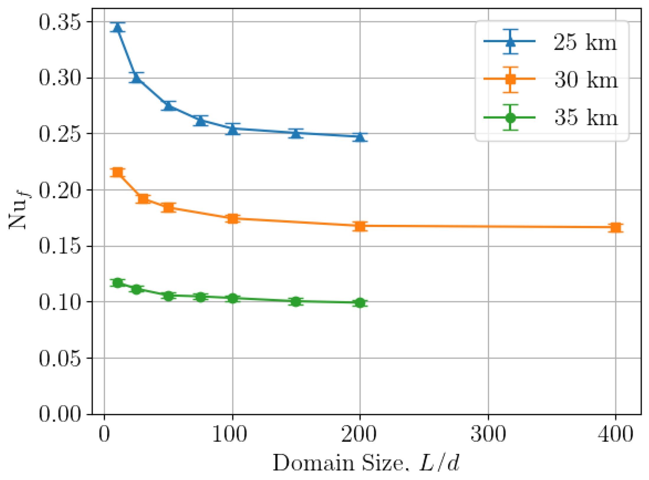
Figure 6.
Comparison of free-molecular theory and experimental data to DSMC results at various pressure values (Knudsen number values). Error bars indicate of the steady-state DSMC data. Dashed vertical lines indicate the approximate Knudsen number values that define the transition-regime.
Figure 6.
Comparison of free-molecular theory and experimental data to DSMC results at various pressure values (Knudsen number values). Error bars indicate of the steady-state DSMC data. Dashed vertical lines indicate the approximate Knudsen number values that define the transition-regime.

Figure 7.
Comparison of DSMC simulation results using two different gas mixtures and experimental data [6]. Error bars indicate of the steady-state DSMC data.
Figure 7.
Comparison of DSMC simulation results using two different gas mixtures and experimental data [6]. Error bars indicate of the steady-state DSMC data.

Figure 8.
Dependence of wire heat transfer on surface accommodation coefficient at different values of wire Knudsen number. Data shown correspond to m/s. Error bars indicate of the steady-state DSMC data.
Figure 8.
Dependence of wire heat transfer on surface accommodation coefficient at different values of wire Knudsen number. Data shown correspond to m/s. Error bars indicate of the steady-state DSMC data.

Figure 9.
Comparison between DSMC results and experimental data [6]. Error bars indicate of the steady-state DSMC data. Shaded regions are predicted uncertainty bounds in the DSMC results due to a ±10% uncertainty in surface accommodation coefficient .
Figure 9.
Comparison between DSMC results and experimental data [6]. Error bars indicate of the steady-state DSMC data. Shaded regions are predicted uncertainty bounds in the DSMC results due to a ±10% uncertainty in surface accommodation coefficient .
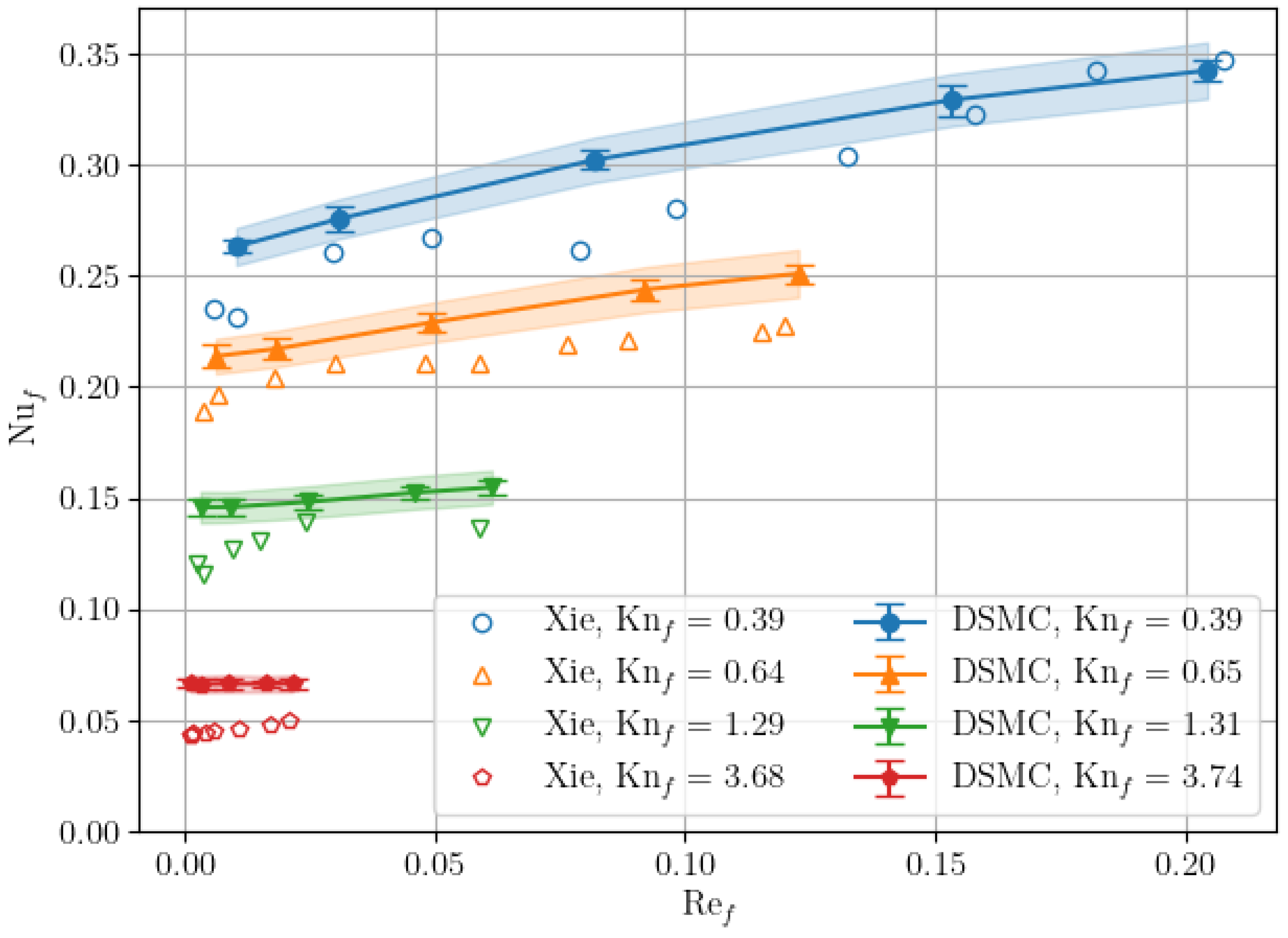
Figure 10.
Simulated wire heat transfer dependence on domain size for the Kn, Re case. Error bars indicate of the steady-state DSMC data. The experimental value from Xie et al. [6] for Kn, Re is also shown.
Figure 10.
Simulated wire heat transfer dependence on domain size for the Kn, Re case. Error bars indicate of the steady-state DSMC data. The experimental value from Xie et al. [6] for Kn, Re is also shown.


Table 1.
Parameters for the variable soft sphere collision model and the Larsen-Borgnakke model used in the current study. is the collision diameter, is the temperature exponent for viscosity, is the reference temperature, is the angular scattering parameter, is the number of rotational degrees of freedom, and is the rotational relaxation number.
| Gas Species | , m | , K | ||||
|---|---|---|---|---|---|---|
| Nitrogen, N | 4.07 | 0.74 | 273.15 | 1.6 | 2 | 0.2 |
| Oxygen, O | 3.96 | 0.77 | 273.15 | 1.4 | 2 | 0.2 |
Table 2.
Knudsen and Reynolds number values for the domain size simulations seen in Figure 5.
Table 2.
Knudsen and Reynolds number values for the domain size simulations seen in Figure 5.
| Altitude, km | Kn | Re |
|---|---|---|
| 25 | 0.50 | 0.0190 |
| 30 | 1.08 | 0.0130 |
| 35 | 2.33 | 0.0039 |
Table 3.
Average uncertainty in DSMC Nu due to a 10% uncertainty in for the four different Knudsen cases seen in Figure 9.
Table 3.
Average uncertainty in DSMC Nu due to a 10% uncertainty in for the four different Knudsen cases seen in Figure 9.
| Kn | |
|---|---|
| 0.39 | 3.4% |
| 0.65 | 4.0% |
| 1.31 | 4.8% |
| 3.74 | 5.7% |
Publisher’s Note: MDPI stays neutral with regard to jurisdictional claims in published maps and institutional affiliations. |
© 2021 by the authors. Licensee MDPI, Basel, Switzerland. This article is an open access article distributed under the terms and conditions of the Creative Commons Attribution (CC BY) license (http://creativecommons.org/licenses/by/4.0/).
Share and Cite
MDPI and ACS Style
Roseman, C.A.; Argrow, B.M. Low-Speed DSMC Simulations of Hotwire Anemometers at High-Altitude Conditions. Fluids 2021, 6, 20. https://doi.org/10.3390/fluids6010020
AMA Style
Roseman CA, Argrow BM. Low-Speed DSMC Simulations of Hotwire Anemometers at High-Altitude Conditions. Fluids. 2021; 6(1):20. https://doi.org/10.3390/fluids6010020
Chicago/Turabian StyleRoseman, Christopher A., and Brian M. Argrow. 2021. "Low-Speed DSMC Simulations of Hotwire Anemometers at High-Altitude Conditions" Fluids 6, no. 1: 20. https://doi.org/10.3390/fluids6010020