Lightning Solvers for Potential Flows


Department of Mathematics, Imperial College London, South Kensington Campus, London SW7 2AZ, UK
Fluids 2020, 5(4), 227; https://doi.org/10.3390/fluids5040227
Submission received: 9 October 2020
/
Revised: 18 November 2020
/
Accepted: 20 November 2020
/
Published: 30 November 2020
(This article belongs to the Special Issue Recent Advances in Fluid Mechanics: Feature Papers)
Abstract
:We present a method for computing potential flows in planar domains. Our approach is based on a new class of techniques, known as “lightning solvers”, which exploit rational function approximation theory in order to achieve excellent convergence rates. The method is particularly suitable for flows in domains with corners where traditional numerical methods fail. We outline the mathematical basis for the method and establish the connection with potential flow theory. In particular, we apply the new solver to a range of classical problems including steady potential flows, vortex dynamics, and free-streamline flows. The solution method is extremely rapid and usually takes just a fraction of a second to converge to a high degree of accuracy. Numerical evaluations of the solutions are performed in a matter of microseconds and can be compressed further with novel algorithms.
1. Introduction
This paper is concerned with the numerical solution of the planar Laplace equation
in contexts relevant to fluid dynamics. The domain D is assumed to be unbounded and simply connected (or periodic) and is the spatial co-ordinate. Laplace’s equation is sometimes considered the simplest two-dimensional (2-D) partial differential equation but, nevertheless, its numerical solution is challenging in many scenarios of practical interest. In particular, typical numerical methods struggle when the boundary of the flow domain is not smooth; for example, the solution of (1) admits a singularity where the boundary has sharp corners [1], which hinders traditional techniques such as finite element methods [2,3] and boundary element methods [4]. Although these approaches have been successfully adapted to account for corners (e.g., [5]), their implementation is complex and requires expert knowledge. Recently, a new method that makes use of rational function approximation theory has been proposed for solving Laplace’s equation in domains with corners [6,7]. Dubbed the “lightning solver” (due to the analogy of lightning striking a corner because of a singular electric potential there), this new solution technique is extremely fast, accurate, and straightforward to implement. Herein, we use the lightning method to devise new strategies for solving potential flow problems in domains with corners.
Potential flows are foundational to fluid mechanics. In the fluid mechanics pedagogy, the first problem that students encounter is often incompressible and irrotational flow past a cylinder. Equipped with the solution to this simple flow, students progress to more complicated geometries via conformal mappings such as the Joukowski map [8]. The ensuing solutions can usually be expressed in closed form and are, thus, highly interpretable. Much of classical aerodynamics was built on this approach [9,10,11] and the associated solutions continue to be relevant to modern aerodynamics studies today [12,13]. Idealised flow also commonly arises as an outer region problem in asymptotic analyses, and can then be matched to an inner boundary layer [14]. Another way to improve the physical fidelity of potential flows is by incorporating the effects of flow separation. The Brown–Michael equation [15] is a popular method for modelling point vortices shed from sharp corners [16,17,18] whereas contour dynamics models the shedding and roll-up of vortex sheets [19,20]. In Section 3.4, we shall see that the lightning approach of the present work can be used to rapidly compute point vortex trajectories in complicated domains. Free-streamline theory [21,22] provides an alternative approach to modelling flow separation; in Section 3.5, we shall use the lightning solver to calculate the idealised, separated flow past a flat plate.
The mathematically tractable structure of potential flows has inspired a rich mathematical theory rooted predominantly in complex analysis. The theory of conformal mappings [23,24,25] has enabled the study of potential flows in complicated domains beyond the aforementioned Joukowski map. Moreover, a theory for multiply connected flow domains has recently been expounded by Crowdy [26,27], and the present author adapted these studies to periodic domains [28]. Both of these approaches make use of the transcendental Schottky–Klein prime function [29]. The prime function also provides a closed-form expression for the Kirchhoff–Routh path function [30], which governs the trajectories of point vortices [31]. Riemann–Hilbert problems and singular integral equations are also relevant, and have previously been used to study flows through cascades [32], porous aerofoils [33], and dissolution and erosion [34].
Corners are obviously ubiquitous in real-life engineering applications and are often responsible for important physical behaviour; the local behaviour of flow past a sharp corner can have a significant impact on the global properties of the flow. For example, the Kutta condition implies that the flow at the sharp trailing edge of an aerofoil should depart the wing smoothly [35]. This specification determines the circulation around the wing and, thus, its lift [36]. At the leading edge of a wing, the leading-edge suction is critical in determining the thrust on unsteady bodies and has recently been proposed as a tool for modelling the onset of vortex shedding [37]. This approach has been coupled with real measurement data in order to account for absent physics via data assimilation to obtain a model that is simultaneously fast and physically faithful [38]. In summary, the flow behaviour at corners must be accurately modelled for physically relevant results.
The remainder of this article is arranged as follows. In Section 2, we explain the lightning solver framework and outline the mathematical details. We then apply this framework to a range of scenarios including potential flows, vortex dynamics, and free-streamline problems in Section 3. Finally, we present a discussion of the results in Section 4. Most of the results that are produced in this paper are computed using straightforward adaptations of the Matlab code laplace.m available at [39]. The reported solve times are based on computations performed on a 2015 MacBook Pro with a 2.9 GHz processor.
2. Method
We now present the main mathematical ideas behind the lightning method.
2.1. The Lightning Method
We are interested in solving Laplace’s equation in an unbounded 2-D domain D with corners on the boundary . Solutions of Laplace’s equation typically exhibit singularities with behaviour near corners; for example, represents the complex potential for flow around an infinite wedge with a corner of interior angle . The absence of viscosity and the infinite curvature of the boundary at the corner imply that the flow there either has infinite velocity or is stagnant. The presence of these singularities suggests that the recently developed lightning solvers can be an efficient and accurate method for computing potential flows.
The ideas behind the lightning method are based in rational approximation theory. A rational function is simply a ratio of two polynomials; we say that a rational function is type if the numerator is a polynomial of degree at most m and the denominator is a polynomial of degree at most n. A detailed discussion of rational approximation can be found in chapters 22 to 27 of [40]. A principal result of rational approximation is due to Newman [41], who showed that the absolute value function can be approximated on the interval with root-exponential accuracy. In mathematical language, there exist constants and type rational approximants such that
In contrast, a polynomial approximant can achieve, at best, algebraic convergence (i.e., the error decays in proportion to ). Motivated by this result, Gopal and Trefethen [6] proved that similar approximants exist for more general types of singularities of the form . Again, it is possible to attain root-exponential convergence when approximating with rational functions; there exist constants and type rational approximants , such that
where H represents the closed upper half of the unit disc. Theorem 2.3 of [6] extended this result to prove that solutions of Laplace’s equation in convex polygons can be represented as rational functions with root-exponential accuracy. Although the theoretical results of [6] were valid when the domain is the interior of a convex polygon, the numerical results of the present paper indicate that they also hold when the domain is the exterior of some bounded domain.
Crucially, the rational approximants in both (2) and (3) possess poles that are exponentially clustered near zero with exponentially decreasing residues. This observation, as well as the above theoretical results, inform a numerical scheme for Laplace’s equation by considering an ansatz with poles clustered exponentially close to the corners of the domain. Gopal and Trefethen [6] suggest an ansatz of the form
where is a point near the center of , is a prescribed set of poles and and are sets of unknown, complex constants. Equation (4) is simply a rational function in partial fraction form. Because rational functions are analytic away from the poles, if all of the poles are outside D then (4) is a solution to Laplace’s equation. The Runge part in (4) corresponds to the smooth part of the solution: it is a polynomial in . If is smooth then the Runge part is all that is necessary in the ansatz. Conversely, the Newman part takes the singularities on the corners into account.
A key feature of the lightning method is that the poles in the Newman part are clustered exponentially close to the corners in order to exploit the root-exponential convergence guaranteed by (3). In particular, there is evidence to suggest that the poles should follow a “tapered” distribution near the corners [42]. In this case, the poles that are clustered around a given corner should be of distance
from that corner. In our numerical results we use although is also a good choice.
By the linearity of Laplace’s equation, the coefficients and can be determined by fitting f to satisfy some prescribed linear boundary conditions. This is achieved by sampling the ansatz (4) at a number of points on the boundary and solving for and in the least-squares sense. The sample points should also be exponentially clustered near the corners in order to ensure that the poles exponentially near the corners are properly resolved. For example, if the boundary condition is collocated at m points then the coefficients are given by
where is the stacked vector of the real and imaginary parts of the unknown coefficients, represents the sampled boundary condition, and represents the sampled basis functions in (4). For example, suppose that the boundary condition is for some function d. Subsequently, for an vector of sample points , we have
where the blocks and correspond to the Runge and Newman parts respectively:
Thus, . It is important to note that the matrix is exponentially ill-conditioned since its columns are the real and imaginary parts of the columns of a Vandermonde matrix. To address this issue, the Vandermonde matrix is not formed explicitly: instead, we form an equivalent matrix with orthogonal columns via the Vandermonde with Arnoldi algorithm [43]. Using these matrix constructions, the least-squares problem (6) can be easily solved using, for example, the backslash operator in Matlab. Having obtained the coefficients and , the rational approximant f can be computed via (4). This completes the description of the lightning solver. Pseudocode describing the main steps is included in Algorithm 1 and we refer the reader to [6] for further details.
| Algorithm 1: Laplace lightning solver (Gopal and Trefethen, 2019 [6]). |
 |
The lightning solver belongs to a broader class of techniques known as Methods of Fundamental Solutions (MFS) [44,45,46]. In these methods, the solution is expanded as a distribution of free-space solutions whose coefficients are tuned to satisfy a given boundary condition. However, the lightning solver differs from typical MFS in two important ways. Firstly, the singularities are exponentially clustered near the corners, which is a new idea in MFS. Secondly, the fundamental solutions that are used here are dipoles (), whereas traditional MFS typically use point sources (). These two qualities are essential to the root-exponential convergence of solutions that we observe herein.
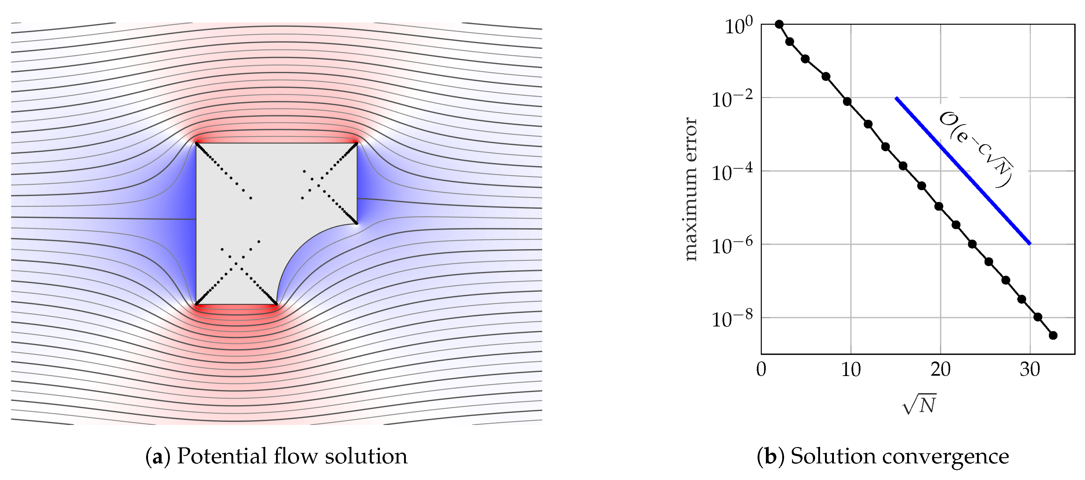
The main idea of this paper is to use the lightning solver to solve potential flow problems. We will apply this approach to a plethora of scenarios to showcase its versatility, but as a first example, consider uniform flow past a stationary boundary . If w represents the complex potential then the no-flux condition states that for and the far-field condition is as . Thus, we may write where f is the ansatz expressed in (4). After arranging the poles to cluster near the corners, the coefficients and are chosen in order to satisfy the no-flux condition. The resulting streamlines are plotted in Figure 1a for a square with a circular sector removed. The background color represents the horizontal perturbation velocity, which can be obtained by differentiating f. In Figure 1b, we plot the convergence of the solution as the number of degrees of freedom () is increased. The problem is solved to six digits of accuracy in 0.5 s. Evaluating the solution takes 20 microseconds for each point. The root-exponential convergence is clear, and the approximation is accurate throughout the entire boundary, including the corners.
2.2. Compression of Solutions
While the rational function representation (4) is very fast to evaluate, even faster evaluations are possible. In certain applications—such as the vortex dynamics example we shall encounter later—the solution f will be evaluated a large number of times and thus an inexpensive evaluation of f is desirable.
Recently, the AAA (adaptive Antoulas–Anderson) algorithm has emerged as a robust, flexible, and accurate tool for rational approximation and compression [47,48]. Given sets of sample points Z and function values , the AAA algorithm returns a rational function r that approximates f to some specified tolerance. One important feature of the AAA algorithm is that the rational function is expressed in barycentric form, i.e.,
The set of support points is a subset of the sample points and are known as the weights. Note that so r interpolates f at the support points. The AAA algorithm selects support points and weights by iteratively reducing the residual error. At each iteration, the next support point is chosen “greedily” as the one with the largest residual error between the approximant and function value. Subsequently, the weight is updated by solving a minimisation problem via a singular value decomposition (SVD). When a desired accuracy is reached then the algorithm terminates—(10) consists of m support points and thus m iterations. These features—the barycentric form, greedy selection of support points and least-squares minimisation via SVD—are all central to the success of the AAA algorithm. The algorithm is straightforward to implement and use: the original article [47] contained an implementation in 40 lines of Matlab code and a full implementation is available in Chebfun [49] (www.chebfun.org). The author has also developed a periodic version of the AAA algorithm, called AAAtrig [50]. The algorithm is built on the same principals as the original AAA algorithm, except the barycentric form (10) is replaced with its periodic analogue.
Let us return to the relevance of AAA to our compression problem. Suppose that we have computed a solution f of the form (4) to Laplace’s equation satisfying some boundary conditions. If we evaluate f at a number of points on the boundary and run these points through the AAA/AAAtrig algorithm then we obtain a new function r that approximates f on the boundary. If r contains no poles in D, then r also solves Laplace’s Equation (1). Moreover, AAA/AAAtrig usually selects an approximation that uses fewer poles than the original function and is, thus, faster to evaluate. Moreover, by the maximum value principle, is maximised on the boundary, so the error in D is guaranteed to be no larger than the approximation error on the boundary.
We illustrate the effects of compression in Figure 2. The problem is uniform flow around a rectangle with a reentrant corner. The lightning solver uses 617 poles to achieve eight digits of accuracy. Figure 2c indicates that the algorithm attains root-exponential convergence. After a sample of the boundary points have been passed through AAA, we obtain a rational approximant using only 412 poles. Thus, the new approximant r is faster to evaluate than the original solution f. Note that AAA has chosen a slightly different set of poles with which to represent the function; we believe that this alternative choice of poles is responsible for the enhanced compression. The idea of compressing harmonic functions using AAA originated in [51].
3. Results and Discussion
Having outlined the mathematical preliminaries of the lightning solver, we now consider a number of fluid dynamics problems.
3.1. Potential Flows
The examples presented in the previous section were for simple uniform flows. The inclusion of more complicated flows follows in an analogous manner. Suppose that a given flow—which may consist of a background flow and a distribution of singularities in D—has a free-space solution . Subsequently, we represent the complex potential as . Thus, is the correction term that is induced by the boundaries and can be found using the methods of Section 2. In order for the boundary to be a streamline, we enforce the boundary condition
For example, suppose that we wish to calculate the potential flow that is generated by a uniform flow of magnitude U at an angle with a distribution of N vortices of circulations at locations . The free-space solution for the complex potential is
The lightning method presented in Section 2 can used to find a harmonic function that satisfies the boundary condition (11). In Figure 3, we visualise the flow past a curved boundary embedded in a uniform flow with two point vortices by plotting a set of streamlines and the horizontal velocity perturbation.
The method is also valid when the boundary is not a streamline. For example, when the boundary is rotating about the point c with angular velocity , (11) is replaced by
3.2. Periodic Domains
Potential flows through periodic domains arise in a number of practical scenarios including turbomachinery flows [32], super-hydrophobic surfaces [53], and geological flows [54]. Recently, the author proposed a “calculus” for the analytical treatment of potential flows in general periodic domains with multiply connected period windows [28] thus extending the calculus of vortex dynamics proposed by Crowdy [27]. The analytical solutions in that work were based on the Schottky–Klein prime function [29]. The present lightning approach may be viewed as a complementary approach to those analytical solutions.
We now seek solutions of Laplace’s equation that are periodic so that for (solutions of different periods can easily be constructed by rescaling the domain). An analogous approach to that of Section 2 can be employed with the ansatz (4) replaced by
The connection between the periodic ansatz (14) and the original ansatz (4) is clarified by noting the partial fraction expansion of cotangent:
Thus, (14) is analogous to (4) when the poles in (4) are repeated with period . Similarly to the non-periodic case, the coefficients and are found by solving the least-squares problem.
In Figure 4 we plot the streamlines and horizontal velocity perturbation for uniform flow at angle past a periodic array of curved boundaries with embedded point vortices. The periodicity has a significant effect on the flow field and the vortices can be seen to deflect the flow angle. At present, this problem cannot be solved with conformal maps, because the form of the required (polycircular) maps has not yet been found. Indeed, the general form of periodic polygonal maps has only been found recently [55]. Accordingly, the lightning approach provides a new method for tackling flows in periodic domains that were previously inaccessible.
3.3. The Kutta Condition
In the lightning ansatz (4), the circulation around is necessarily zero. It is possible to give arbitrary circulation by replacing the ansatz (4) with
and solving for and subject to the relevant boundary condition. However, in most applications, the circulation is not prescribed, but must be found as part of the problem. One method for selecting the circulation is to apply the Kutta condition [35,36]. On , a corner is nominated as the downstream corner and the Kutta condition states that the fluid should leave smoothly. In our potential flow framework (for a stationary boundary), this is equivalent to specifying that the corner represents a stagnation point. In other words, the circulation must be such that the velocity vanishes at the nominated corner, i.e.,
where g is the free-space solution and the prime ′ indicates differentiation with respect to z. Practically, enforcing the Kutta condition simply involves supplementing the least-squares problem (6) with an extra row corresponding to the vectorised form of (17). Note that only one extra row is required as (17) is already satisfied in one direction by the no-flux condition.
In Figure 5, we illustrate the effect of the Kutta condition by computing the uniform flow past a bullet-shaped object with and without the Kutta condition applied. Applying the Kutta condition to the bottom right corner drastically increases the flow velocity in the vicinity of the boundary. It can be seen that the flow departs the selected corner smoothly, thus indicating that the Kutta condition is indeed satisfied.
3.4. Vortex Dynamics
The transport of vortical structures is an important phenomenon in fluid mechanics and is relevant to flow control, turbulence modelling, vortex shedding, and flow separation. A point vortex may be used in order to represent a discretised quantity of vorticity as an approximation to more complicated structures [56]. The dynamics of these point vortices—which has been described as “a classical mathematics playground” [57]—is another area that is amenable to these lightning methods.
The point vortex equation states that the velocity of a vortex is equal to the de-singularised velocity field at the vortex center [58]. Mathematically, if z is the position of a vortex of circulation , then the motion of the vortex is governed by
where w is the complex potential and is the complex velocity. In (18), the tilde indicates that the velocity field has been de-singularised, i.e.,
Accordingly, if we know the velocity field w when the vortex is at z then we can calculate the trajectory of the vortex. We could, in principle, use the lightning method of Section 3.1 to directly calculate w at each time step, but, since the vortices are moving, this approach would require solving a different Laplace problem at each time step, which would become prohibitively expensive. Nevertheless, we can still use the lightning framework to attack this problem.
Our approach is to use the lightning solver to conformally map the physical domain to a simple domain and then analytically construct w with the method of images. There are a number of techniques available that can be used to compute conformal mappings. The pre-eminent method is the Schwarz–Christoffel transformation [23,55,59] which provides analytical formulae for conformal maps to polygonal domains in terms of a number of accessory parameters that must generally be determined numerically. To circumvent this “parameter problem”, an approach for numerically computing conformal maps was suggested in [60]; we briefly review the approach here.
In the simply connected case, the natural domain to map into is the interior of the unit disc. We denote the unit disc coordinate as and the conformal map f, so that . Figure 6 illustrates an example of a mapping. The inverse map (from the physical domain to the circular domain) is written as , so that .
To compute the mappings we express the inverse map as
for analytic h. Taking the logarithm of both sides and evaluating on the boundary yields
where we have used the fact that the boundary maps to . Note that the logarithm on the left side is pure imaginary since we are evaluating it on the unit circle. This imaginary function is unknown as we do not know the image of each boundary point a priori; we only know that the boundary is mapped to the unit circle. Accordingly, to determine , we must find an analytic function who’s real part satisfies (21). In other words, we want to solve the Laplace problem
The last equation specifies a degree of freedom in the map and simplifies some of the ensuing formulae. This type of Laplace problem is amenable to the method that is presented in Section 2: we consider an ansatz in the form of a rational function (4) with poles clustered near the corners and then solve for the coefficients in the least-squares sense by collocating (23) on the boundary. Given h, we obtain by (20).
Now, we may compute the forward mapping f using the approach of [51]. By sampling at a number of points on the boundary , we are equipped with a set of sample points and a set of function values where . Subsequently we construct an approximant with the AAA algorithm using as function values and as sample points. Thus, provided a rich enough sample set is selected, the approximant produced by AAA maps the boundary to ; in other words, the new approximant computed by AAA approximates the forward mapping f. Moreover, by the maximum value principle, the accuracy of the approximation to the conformal map is bounded by the error on the boundary. Accordingly, we are now free to accurately and quickly map between the circular and physical domains using f and .
Armed with these numerical representations of the mappings, we now transform the point vortex Equation (18) into the circular domain . Carefully applying L’Hôpital’s rule to (18) yields
where is the complex potential in and is the de-singularised velocity field in :
The advantage of our approach is that the complex potential in the -plane can be constructed analytically. For example, the complex potential that is induced by an arrangement of N vortices of strengths located at positions embedded in a background uniform flow of strength U at angle of attack is given by
where is the residue of the simple pole of the map. In this case, the de-singularised velocity at is
Substituting (28) into the transformed point vortex equation (25) results in an autonomous dynamical system that can be integrated with standard numerical techniques such as the Euler method or Runge–Kutta methods. In Figure 7, the resulting trajectories are plotted for 30 vortices outside a curved domain. The vortices have strengths that are randomly distributed in the interval [−1, 1] and there is no background flow. A number of vortices are shot out to infinity, but a distinct structure emerges that traces out the boundary . This model could be used as, for example, an approximation for the motion of oceanic eddies [17] around a boundary. Alternatively, on use of the Blasius theorem, this model could provide estimates for the forces exerted on due to the transport of vorticity. The sound produced by such interactions could be also analysed with the vortex sound model of Howe [61].
This approach also applies to multiply connected domains—the analogous complex potential (27) can be constructed in a multiply connected circular domain using the formulae of Crowdy [26,27]. Additionally, this conformal mapping method can be applied to Kirchhoff–Routh theory to study the Hamiltonian dynamics of point vortices [58,62]. Again, analytic formulae for the multiply connected Kirchhoff–Routh path function are readily available [31]. A further consideration is that, in reality, a number of vortices will be shed from the sharp corners of the domain. The trajectories of these shed vortices could be modelled using the Brown–Michael equation [15] or the other approaches discussed in the introduction.
3.5. Free-Streamline Flows
Incompressible flow past a bluff body usually results in flow separation. This separation can generate a downstream wake or a cavity flow and can have a significant effect on estimates of the drag and lift coefficients. Free-streamline theory attempts to reconcile the physical reality of flow separation with the mathematical tractability of potential flows. In these problems, the boundaries of the domain are not known a priori—the boundary incorporates a “free streamline” whose shape must be found as part of the problem. Thus, we cannot use a direct conformal mapping approach as in Section 3.4. The typical approach for solving these problems is to construct mappings between auxiliary domains and then find the shape of the streamlines by considering the relationships between the auxiliary domains. Previous authors have presented numerical conformal mapping approaches in order to solve these problems [22,63,64]; we now demonstrate that the lightning approach can be leveraged in order to solve free-streamline problems.
We consider a rigid body immersed in a separated flow that is uniform in the far-field. The goal is to calculate the velocity field induced by the boundary and the shape of the separation region behind the body. As before, we define the complex potential as and the complex velocity as . In this situation, enforcing the Kutta condition specifies that the flow detaches from the solid body at the edges. We assume that the fluid inside the separation region is stagnant and it is therefore of constant pressure. The free streamlines are the curves that divide the moving fluid from the stagnant fluid; therefore, they represent an infinitesimal shear layer. Because there can be no pressure jump either side of shear layer, the pressure along the free streamline must be constant. Accordingly, Bernoulli’s theorem implies that (subject to a suitable scaling) the speed of fluid along the boundary of the wake is unity:
Furthermore, the no-flux condition specifies that, on the surface of the solid body, the fluid velocity must be tangent to the boundary:
where s is the arc length of the boundary.
The streamfunction is piecewise constant on both the rigid boundary and the free streamlines. We say ‘piecewise constant’ here, because there may be multiple free streamlines that correspond to different values of the streamfunction. Since both w and are analytic functions in simply connected domains, and assuming that they have a 1-to-1 relation, there exists a conformal map f between them:
We can now connect the physical coordinate z to the complex potential w and complex velocity by
The above maps a complex velocity value () to a physical coordinate (z). Thus, if f can be determined, then we know z and the corresponding velocity value there. The boundary conditions on f follow from (29) and (30), as
The precise constants that attains on the boundaries are application dependent.
The problem of finding an analytic function f subject to the boundary conditions (33) may be solved using the lightning method introduced in Section 2. The lightning method is very appropriate to this problem, because the domain typically contains corners even though the physical z domain does not. While conventional methods struggle to resolve the singularities at the corners, the lightning method achieves root-exponential convergence.
In Figure 8, we illustrate the procedure for the separated flow past a flat plate. The incoming flow is inclined at an angle of . Along the free streamline, the velocity has magnitude 1 and along the plate the flow has zero normal velocity. Accordingly, the flow domain in the domain is a semicircle. We use the lightning method to compute the mapping from the complex velocity () domain to the complex potential domain (w), such that the semicircle is a streamline and the point maps to infinity. Poles are clustered exponentially close to the corners of the semicircle in order to exploit the root-exponential convergence afforded by rational function approximation. In the complex potential domain, the boundaries are the upper and lower parts of the positive real axis. Having computed f, we may then use (32) to establish the relationship between the velocity and the spatial position z, which is plotted at the bottom of Figure 8. This problem can actually be solved analytically by appropriately placing image doublets in the domain, but the example is included here in order to illustrate the applicability of the lightning solver to free-streamline flows.
There are several methods available for improving the physical fidelity of free-streamline theory, the most conspicuous of which is the approach of Wu [21]. By allowing the pressure on the free streamline to increase monotonically, Wu [21] ensures that the free streamlines become asymptotically parallel to the background flow at infinity. This yields favourable comparisons for the lift and drag coefficients against experimental results. The simple example that we have presented does not allow the pressure on the free streamline to vary, but this effect could be incorporated to improve the realism of the model.
4. Conclusions
In this paper we have presented a new method for numerically solving potential flow problems. Our method is based on the lightning method introduced by Gopal and Trefethen [6,7], and exploits the approximation power of rational functions. We believe that the technique will be useful to researchers in fluid mechanics who wish to quickly compute solutions to potential flows with modest accuracy in domains that prohibit fully analytical solutions and traditional numerical methods. The technique is comparatively simple and does not require specialised knowledge of finite element methods or boundary element methods. We have demonstrated that the method is valuable for several physical problems, including steady potential flows, unsteady vortex dynamics, and free streamline flows. Periodic domains are not an issue and are handled with a slightly different ansatz. The solutions converge extremely fast (with root-exponential convergence) and are themselves very fast to evaluate. When the solution is to be evaluated a large number of times, such as in the vortex dynamics simulations presented in Section 3.4, the solutions can be compressed using the AAA or AAAtrig algorithms.
Potential flows are mathematically elegant but neglect important physical phenomena. We have suggested two approaches to ameliorate these effects by incorporating vortex dynamics (Section 3.4) and flow separation (Section 3.5). The approach has also been demonstrated to apply to the Helmholtz equation [7], which could prove useful for acoustics and aeroacoustics problems. Additionally, there is the exciting possibility of extending the lightning solver to 3-D; apart from the conformal mapping of Section 3.4, our approach did not use complex variables except as a convenient coordinate system. This is a topic to be pursued in future studies.
Funding
This research was supported by an EPSRC Doctoral Prize from Imperial College London.
Acknowledgments
The author acknowledges the 2019 Fluids Travel Award from MDPI that supported attendance at the 2019 APS DFD meeting where some of the ideas in this paper were generated.
Conflicts of Interest
The author declares no conflict of interest.
References
- Lehman, R. Developments at an analytic corner of solutions of elliptic partial differential equations. Indiana Univ. Math. J. 1959, 8, 727–760. [Google Scholar] [CrossRef]
- Arndt, D.; Bangerth, W.; Blais, B.; Clevenger, T.C.; Fehling, M.; Grayver, A.V.; Heister, T.; Heltai, L.; Kronbichler, M.; Maier, M.; et al. The deal.II library, Version 9.2. J. Numer. Math. 2020, 28, 131–146. [Google Scholar] [CrossRef]
- Logg, A.; Mardal, K.A.; Wells, G.N. Automated Solution of Differential Equations by the Finite Element Method; Lecture Notes in Computational Science and Engineering; Springer: Berlin/Heidelberg, Germany, 2012; Volume 84 LNCSE, pp. 1–736. [Google Scholar] [CrossRef]
- Aliabadi, M.H.; Wen, P.H. Boundary element methods in engineering course. Eng. Anal. 1984, 1, 61–62. [Google Scholar] [CrossRef]
- Serkh, K.; Rokhlin, V. On the solution of elliptic partial differential equations on regions with corners. J. Comput. Phys. 2016, 305, 150–171. [Google Scholar] [CrossRef] [Green Version]
- Gopal, A.; Trefethen, L.N. Solving Laplace problems with corner singularities via rational functions. SIAM J. Numer. Anal. 2019, 57, 2074–2094. [Google Scholar] [CrossRef]
- Gopal, A.; Trefethen, L.N. New Laplace and Helmholtz solvers. Proc. Natl. Acad. Sci. USA 2019, 116, 10223–10225. [Google Scholar] [CrossRef] [PubMed] [Green Version]
- Joukowski, N. Über die Konturen der Tragflächen der Drachenflieger. Z. Flugtech. Mot. 1910, 1, 281–284. [Google Scholar]
- Theodorsen, T. General Theory of Aerodynamic Instability and the Mechanism of Flutter; National Aeronautics and Space Administration: Washington, DC, USA, 1979; pp. 291–311.
- Sears, W.R. Some Aspects of Non-Stationary Airfoil Theory and Its Practical Application. J. Aeronaut. Sci. 1941, 8, 104–108. [Google Scholar] [CrossRef]
- Wu, T.Y.T. Swimming of a waving plate. J. Fluid Mech. 1961, 10, 321–344. [Google Scholar] [CrossRef]
- Cordes, U.; Kampers, G.; Meiner, T.; Tropea, C.; Peinke, J.; Hölling, M. Note on the limitations of the Theodorsen and Sears functions. J. Fluid Mech. 2017, 811, R11–R111. [Google Scholar] [CrossRef]
- Wei, N.J.; Kissing, J.; Wester, T.T.; Wegt, S.; Schiffmann, K.; Jakirlic, S.; Hölling, M.; Peinke, J.; Tropea, C. Insights into the periodic gust responseA ofA airfoils. J. Fluid Mech. 2019, 876, 237–263. [Google Scholar] [CrossRef] [Green Version]
- Van Dyke, M. Perturbation Methods in Fluid Mechanics; Academic Press: New York, NY, USA, 1964. [Google Scholar]
- Brown, C.E.; Michael, W.H. Effect of leading-edge separation on the lift of a delta wing. J. Aeronaut. Sci. 1954, 21, 690–694. [Google Scholar] [CrossRef]
- Michelin, S.; Llewellyn Smith, S.G. An unsteady point vortex method for coupled fluid-solid problems. Theor. Comput. Fluid Dyn. 2009, 23, 127–153. [Google Scholar] [CrossRef] [Green Version]
- Southwick, O.R.; Johnson, E.R.; McDonald, N.R. A point vortex model for the formation of ocean eddies by flow separation. Phys. Fluids 2015, 27, 16604. [Google Scholar] [CrossRef] [Green Version]
- Manela, A.; Halachmi, M. Mechanisms of sound amplification and sound reduction in the flapping flight of side-by-side airfoils. J. Sound. Vib. 2015, 346, 216–228. [Google Scholar] [CrossRef]
- Pullin, D. Contour Dynamics Methods. Annu. Rev. Fluid Mech. 1992, 24, 89–115. [Google Scholar] [CrossRef]
- Krasny, R. Desingularization of periodic vortex sheet roll-up. J. Comput. Phys. 1986, 65, 292–313. [Google Scholar] [CrossRef]
- Wu, T.Y.T. A wake model for free-streamline flow theory: Part 1. Fully and partially developed wake flows past an oblique flat plate. J. Fluid Mech. 1962, 13, 161–181. [Google Scholar] [CrossRef]
- Hassenpflug, W.C. Free-streamlines. Comput. Math. Appl. 1998, 36, 69–129. [Google Scholar] [CrossRef] [Green Version]
- Driscoll, T.A.; Trefethen, L.N. Schwarz-Christoffel Mapping; Cambridge University Press: Cambridge, UK, 2002. [Google Scholar]
- Crowdy, D.G.; Marshall, J. Conformal mappings between canonical multiply connected domains. Comput. Methods Funct. Theory 2006, 6, 59–76. [Google Scholar] [CrossRef]
- Nehari, Z. Conformal Mapping; McGraw-Hill: New York, NY, USA, 1952. [Google Scholar]
- Crowdy, D.G. Solving problems in multiply connected domains. In SIAM CBMS-NSF Regional Conference Series in Applied Mathematics; SIAM: Philadelphia, PA, USA, 2020. [Google Scholar]
- Crowdy, D.G. A new calculus for two-dimensional vortex dynamics. Theor. Comput. Fluid Dyn. 2010, 24, 9–24. [Google Scholar] [CrossRef]
- Baddoo, P.J.; Ayton, L.J. A calculus for flows in periodic domains. Theor. Comput. Fluid Dyn. 2020, arXiv:2001.00859. [Google Scholar] [CrossRef]
- Crowdy, D.G.; Kropf, E.H.; Green, C.C.; Nasser, M.M.S. The Schottky-Klein prime function: A theoretical and computational tool for applications. IMA J. Appl. Math. 2016, 81, 589–628. [Google Scholar] [CrossRef] [Green Version]
- Lin, C.C. On the motion of vortices in two dimensions: I. Existence of the Kirchhoff–Routh function. Proc. Natl. Acad. Sci. USA 1941, 27, 575–577. [Google Scholar] [CrossRef] [PubMed] [Green Version]
- Crowdy, D.G.; Marshall, J. Analytical formulae for the Kirchhoff-Routh path function in multiply connected domains. Proc. R. Soc. A Math. Phys. Eng. Sci. 2005, 461, 2477–2501. [Google Scholar] [CrossRef]
- Baddoo, P.J.; Ayton, L.J. Potential flow through a cascade of aerofoils: Direct and inverse problems. Proc. R. Soc. A Math. Phys. Eng. Sci. 2018, 474, 20180065. [Google Scholar] [CrossRef] [Green Version]
- Hajian, R.; Jaworski, J.W. The steady aerodynamics of aerofoils with porosity gradients. Proc. R. Soc. A Math. Phys. Eng. Sci. 2017, 473, 20170266. [Google Scholar] [CrossRef]
- Moore, M.N.J. Riemann–Hilbert problems for the shapes formed by bodies dissolving, melting, and eroding in fluid flows. Commun. Pure Appl. Math. 2017, 70, 1810–1831. [Google Scholar] [CrossRef]
- Crighton, D.G. The Kutta condition in unsteady flow. Annu. Rev. Fluid Mech. 1985, 17, 411–445. [Google Scholar] [CrossRef]
- Eldredge, J.D. Mathematical Modeling of Unsteady Inviscid Flows; Interdisciplinary Applied Mathematics; Springer International Publishing: New York, NY, USA, 2019; Volume 50, p. 461. [Google Scholar] [CrossRef]
- Ramesh, K.; Gopalarathnam, A.; Granlund, K.; Ol, M.V.; Edwards, J.R. Discrete-vortex method with novel shedding criterion for unsteady aerofoil flows with intermittent leading-edge vortex shedding. J. Fluid Mech. 2014, 751, 500–538. [Google Scholar] [CrossRef]
- Darakananda, D.; da Silva, A.F.d.C.; Colonius, T.; Eldredge, J.D. Data-assimilated low-order vortex modeling of separated flows. Phys. Rev. Fluids 2018, 3, 124701. [Google Scholar] [CrossRef]
- Trefethen, L.N. Lightning Laplace Software. 2020. Available online: https://people.maths.ox.ac.uk/trefethen/lightning (accessed on 21 November 2020).
- Trefethen, L.N. Approximation Theory and Approximation Practice, Extended Edition; SIAM: Philadelphia, PA, USA, 2019. [Google Scholar]
- Newman, D.J. Rational approximation to |x|. Mich. Math. J. 1964, 11, 11–14. [Google Scholar] [CrossRef]
- Trefethen, L.N.; Nakatsukasa, Y.; Weideman, J.A.C. Exponential Node Clustering at Singularities for Rational Approximation, Quadrature, and PDEs. Numer. Math. 2020, in press. [Google Scholar]
- Brubeck, P.D.; Nakatsukasa, Y.; Trefethen, L.N. Vandermonde with Arnoldi. SIAM Rev. 2020, in press. [Google Scholar]
- Fairweather, G.; Karageorghis, A. The method of fundamental solutions for elliptic boundary value problems. Adv. Comput. Math. 1998, 9, 69–95. [Google Scholar] [CrossRef]
- Mathon, R.; Johnston, R.L. The approximate solution of elliptic boundary-value problems by fundamental solutions. SIAM J. Numer. Anal. 1977, 14, 638–650. [Google Scholar] [CrossRef]
- Kupradze, V.D.; Aleksidze, M.A. The method of functional equations for the approximate solution of certain boundary value problems. USSR Comput. Math. Math. Phys. 1964, 4, 82–126. [Google Scholar] [CrossRef]
- Nakatsukasa, Y.; Sète, O.; Trefethen, L.N. The AAA algorithm for rational approximation. SIAM J. Sci. Comput. 2018, 40, A1494–A1522. [Google Scholar] [CrossRef]
- Nakatsukasa, Y.; Trefethen, L.N. An algorithm for real and complex rational minimax approximation. SIAM J. Sci. Comput. 2020, 42, A3157–A3179. [Google Scholar] [CrossRef]
- Driscoll, T.A.; Hale, N.; Trefethen, L.N. Chebfun Guide; Pafnuty Publications: Oxford, UK, 2014. [Google Scholar]
- Baddoo, P.J. The AAAtrig algorithm for rational approximation of periodic functions. arXiv 2020, arXiv:2008.05446. [Google Scholar]
- Gopal, A.; Trefethen, L.N. Representation of conformal maps by rational functions. Numer. Math. 2019, 142, 359–382. [Google Scholar] [CrossRef] [Green Version]
- Howell, L.H. Numerical conformal mapping of circular arc polygons. J. Comput. Appl. Math. 1993, 46, 7–28. [Google Scholar] [CrossRef] [Green Version]
- Crowdy, D.G. Effective slip lengths for immobilized superhydrophobic surfaces. J. Fluid Mech. 2017, 825, R2. [Google Scholar] [CrossRef] [Green Version]
- Vasconcelos, G.L. Multiple bubbles and fingers in a Hele-Shaw channel: Complete set of steady solutions. J. Fluid Mech. 2015, 780, 299–326. [Google Scholar] [CrossRef] [Green Version]
- Baddoo, P.J.; Crowdy, D.G. Periodic Schwarz–Christoffel mappings with multiple boundaries per period. Proc. R. Soc. A 2019, 475. [Google Scholar] [CrossRef] [Green Version]
- Llewellyn Smith, S.G. How do singularities move in potential flow? Phys. D Nonlinear Phenom. 2011, 240, 1644–1651. [Google Scholar] [CrossRef] [Green Version]
- Aref, H. Point vortex dynamics: A classical mathematics playground. J. Math. Phys. 2007, 48, 065401. [Google Scholar] [CrossRef] [Green Version]
- Saffman, P.G. Vortex Dynamics; Cambridge University Press: Cambridge, UK, 1993. [Google Scholar]
- Crowdy, D.G. The Schwarz–Christoffel mapping to bounded multiply connected polygonal domains. Proc. R. Soc. A Math. Phys. Eng. Sci. 2005, 461, 2653–2678. [Google Scholar] [CrossRef]
- Trefethen, L.N. Numerical conformal mapping with rational functions. Comput. Methods Funct. Theory 2020, 20, 369–387. [Google Scholar] [CrossRef]
- Howe, M.S. Theory of Vortex Sound; Cambridge University Press: Cambridge, UK, 2003; p. 216. [Google Scholar]
- Lin, C.C. On the Motion of Vortices in Two Dimensions: II. Some Further Investigations on the Kirchhoff-Routh Function. Proc. Natl. Acad. Sci. USA 1941, 27, 575–577. [Google Scholar] [CrossRef] [PubMed] [Green Version]
- Elcrat, A.R.; Trefethen, L.N. Classical free-streamline flow over a polygonal obstacle. J. Comput. Appl. Math. 1986, 14, 251–265. [Google Scholar] [CrossRef] [Green Version]
- Hureau, J.; Brunon, E.; Legallais, P. Ideal free streamline flow over a curved obstacle. J. Comput. Appl. Math. 1996, 72, 193–214. [Google Scholar] [CrossRef] [Green Version]
Figure 1.
Incompressible, irrotational (i.e., potential) flow past a square circular sector removed. The problem takes 0.5 s to solve to six digits of accuracy and 5 s for eight digits. In (a) the black dots represent the poles. The background colour in (a) represents the horizontal velocity of the perturbation to the flow from uniformity. Note that in (b) the y-axis is on a log scale whereas the x-axis is , so that a straight line indicates root-exponential convergence.

Figure 2.
An example of AAA compression for the flow past a rectangle with a reentrant corner. The black dots in (a) and (b) indicate the poles used to represent the full and compressed solutions respectively.
Figure 2.
An example of AAA compression for the flow past a rectangle with a reentrant corner. The black dots in (a) and (b) indicate the poles used to represent the full and compressed solutions respectively.

Figure 3.
Uniform flow past the polycircular domain from [52] with embedded point vortices. The lines are the streamlines and background color is the horizontal perturbation velocity. The black dots represent the prescribed poles of the rational function. The solution converges to five digits of accuracy in 0.8 s and 8 digits in 6 s.

Figure 4.
Uniform flow past a periodic array of boundaries with embedded point vortices. The black dots represent the prescribed poles of the rational function. The solution converges to 9 digits of accuracy in 0.8 s.
Figure 4.
Uniform flow past a periodic array of boundaries with embedded point vortices. The black dots represent the prescribed poles of the rational function. The solution converges to 9 digits of accuracy in 0.8 s.

Figure 5.
An illustration of the effects of the Kutta condition on the flow past a bullet-shaped object. The solutions are computed to 6 digits of accuracy; in (a) the solver takes 0.3 s and in (b) the solver takes 0.8 s. The color scale is the same in both figures.
Figure 5.
An illustration of the effects of the Kutta condition on the flow past a bullet-shaped object. The solutions are computed to 6 digits of accuracy; in (a) the solver takes 0.3 s and in (b) the solver takes 0.8 s. The color scale is the same in both figures.

Figure 6.
An example of a conformal map computed using the method of [60]. The red dots indicate the poles of the map and their size is proportional to their residue.
Figure 6.
An example of a conformal map computed using the method of [60]. The red dots indicate the poles of the map and their size is proportional to their residue.

Figure 7.
The trajectories of 30 vortices computed with the lightning method. The circulations of the vortices are randomly distributed in the interval . The initial positions of the vortices are equispaced on a circle, as indicated by the coloured dots. The background flow is set to .
Figure 7.
The trajectories of 30 vortices computed with the lightning method. The circulations of the vortices are randomly distributed in the interval . The initial positions of the vortices are equispaced on a circle, as indicated by the coloured dots. The background flow is set to .

Figure 8.
The separated flow past a flat plate at angle of attack . The lines are the streamlines and the colour represents the vertical velocity component.
Figure 8.
The separated flow past a flat plate at angle of attack . The lines are the streamlines and the colour represents the vertical velocity component.

Publisher’s Note: MDPI stays neutral with regard to jurisdictional claims in published maps and institutional affiliations. |
© 2020 by the author. Licensee MDPI, Basel, Switzerland. This article is an open access article distributed under the terms and conditions of the Creative Commons Attribution (CC BY) license (http://creativecommons.org/licenses/by/4.0/).
Share and Cite
MDPI and ACS Style
Baddoo, P.J. Lightning Solvers for Potential Flows. Fluids 2020, 5, 227. https://doi.org/10.3390/fluids5040227
AMA Style
Baddoo PJ. Lightning Solvers for Potential Flows. Fluids. 2020; 5(4):227. https://doi.org/10.3390/fluids5040227
Chicago/Turabian StyleBaddoo, Peter J. 2020. "Lightning Solvers for Potential Flows" Fluids 5, no. 4: 227. https://doi.org/10.3390/fluids5040227