Numerical Investigation of the Cavitation Effects on the Vortex Shedding from a Hydrofoil with Blunt Trailing Edge


Departament de Mecànica de Fluids, Universitat Politècnica de Catalunya, 08028 Barcelona, Spain
*
Author to whom correspondence should be addressed.
Fluids 2020, 5(4), 218; https://doi.org/10.3390/fluids5040218
Submission received: 20 October 2020
/
Revised: 18 November 2020
/
Accepted: 19 November 2020
/
Published: 21 November 2020
(This article belongs to the Special Issue Cavitating Flows)
Abstract
:Vortex cavitation can appear in the wake flow of hydrofoils, inducing unwanted consequences such as vibrations or unstable behaviors in hydraulic machinery and systems. To investigate the cavitation effects on hydrofoil vortex shedding, a numerical investigation of the flow around a 2D NACA0009 with a blunt trailing edge at free caviation conditions and at two degrees of cavitation developments has been carried out by means of the Zwart cavitation model and the LES WALE turbulence model which permits predicting the laminar to turbulent transition of the boundary layers. To analyze the dynamic behavior of the vortex shedding process and the coherent structures, two identification methods based on the Eulerian and Lagrangian reference frames have been applied to the simulated unsteady flow field. It is found that the cavitation occurrence in the wake significantly changes the main vortex shedding characteristics including the morphology of the vortices, the vortex formation length, the effective height of the near wake flow and the shedding frequency. The numerical results predict that the circular shape of the vortices changes to an elliptical one and that the vortex shedding frequency is significantly increased under cavitation conditions. The main reason for the frequency increase seems to be the reduction in the transverse separation between the upper and lower rows of vortices induced by the increase in the vortex formation length.
1. Introduction
In recent decades, the interaction effects between cavitation and vortical flow structures have attracted great attention in academic research and engineering practice. The high vorticity intensity in the center of a vortical flow generates a low-pressure region which is prone to cavitation inception [1,2]. Furthermore, this type of cavitation is affected by vorticity generation mechanisms [3]. Once a cavitation bubble is formed and develops inside the vortex core, the unsteady vortex dynamic behavior, e.g., vortex shedding frequency and vortex formation length, tend to change significantly [4]. As cavitation is further developed, it may give rise to vibrations, noise and material erosion which is an actual risk for the safe operation of hydraulic machinery and systems [1].
To distinguish vortical flow cavitation and the cavitation appearing in a shear flow induced by a high-speed submerged jet, so-called jet cavitation, the cavitation in the vortices generated in the wake of the flow around a bluff body wake is called wake cavitation [2]. Many experimental and numerical research works can be found treating wake vortices behind bluff bodies in single-phase flows, like behind a circular cylinder [5,6,7] and a 2D wedge [8,9], which permit explaining the alternate vortex shedding mechanism. Although some researchers have also paid attention to the cavitating flow behind a circular cylinder [10,11,12,13] and a 2D wedge [3,4,14,15,16,17,18], there is a lack of investigations devoted to understanding the cavitation effects on the dynamics of wake vortices, especially behind 2D symmetric hydrofoils.
Young and Holl [14] were the first to experimentally measure the vortex shedding frequency behind a 2D triangular wedge. They found that the vortex shedding frequency remains constant when cavitation appears at cavitation number σi, but as the cavitation number σ further decreases below σi and the cavitation size increases, the vortex shedding frequency suffers an abrupt rise near ½ of σi. After the vortex shedding frequency reaches this maximum value and σ is further decreased, the individual cavitation vortices grow until the point that they suffer a coalescence and it becomes impossible to measure any shedding frequency. Rao and Chandrasekhara [11] and Ramamurthy [12,15,19] also observed and confirmed similar results both in a circular cylinder and triangular wedge geometry under different area ratios of the model to the test section. Based on high-speed imaging results, Belahadji [4] found that cavitation cannot be considered as irrelevant for the flow around a 2D wedge since, as soon as cavitation happens, it can dramatically change the flow dynamics and lead to an increase in the vortex shedding frequency. However, this behavior is not often mentioned in research devoted to the observation and characterization of wake cavitation behind 2D symmetric hydrofoils. Ausoni et al. [20] conducted an experimental research to determine the cavitation effects on the flow behind a truncated NACA 0009 hydrofoil at high Reynolds numbers. With a high-speed camera and a laser vibrometer, they confirmed that the vortex shedding frequency increased gradually with the development of cavitation, although no mechanism for the phenomena was thoroughly described.
An important parameter that determines the vortex shedding frequency at the high Reynolds numbers is the vortex formation length as proposed by Gerrard [5]. In a single-phase flow, Gerrard insisted that the larger the vortex formation region, the lower the vortex shedding frequency. However, when cavitation occurs, the situation becomes more complex. For example, Kumar et al. [21] observed and confirmed similar results at subcritical Reynolds numbers on the cavitating flow over a circular cylinder employing high-speed imaging. In contrast, Ramamurthy et al. [12] observed an increase in the vortex formation length when σ decreased in both a 2D wedge and a circular cylinder. Despite those works, few studies can be found related to the vortex formation length behind hydrofoils. Ausoni et al. [20] provided measurements of the vortex formation length for different free stream velocities at cavitation free regimes. They concluded that the vortex shedding frequency is reduced as the vortex formation length increases both in the natural boundary layer transition and tripped transition setups, which agrees well with Gerrard [5]. Nevertheless, no measurements of the vortex formation length for cavitation conditions were reported in their study.
Some numerical investigations regarding the vortex shedding flow around hydrofoils without cavitation should be mentioned. Ausoni et al. [20] carried out a numerical investigation of the vortex shedding behind a NACA 0009 hydrofoil with a truncated trailing edge for several free stream velocities and high Reynolds numbers under no cavitation conditions. Their numerical results showed that the boundary layer transition from laminar to turbulent regimes predicted with the SST transition turbulence model provided more consistent results with the experimental measurements than the standard SST turbulence model. Lee et al. [22] and Chen et al. [23] used 2D LES and 3D LES turbulence models, respectively, to investigate the same hydrofoil geometry. They stated that the choice of a turbulent model with the capability of predicting the boundary layer laminar to turbulence transition is a key point to obtain an accurate prediction of the vortex shedding frequency.
Under cavitation conditions, the most commonly used cavitation model is the homogeneous mixture model, which is derived from the simplified Rayleigh–Plesset bubble dynamics equation. The coupling of the cavitation model with RANS and LES turbulence models has been found to capture with good accuracy the cavitating flow phenomena in the wake of bluff bodies. For example, Kim et al. [24] used a combination of URANS with a homogeneous mixture cavitation model to investigate the unsteady cavitating flow over a 2D triangular wedge. Further, Gnanaskandan et al. [13,17] applied the LES turbulence model coupled with a compressible homogeneous mixture cavitation model to investigate the cavitating wake flow over a circular cylinder and a 2D wedge. In summary, these numerical investigations confirmed the capability of the homogeneous mixture cavitation models to predict the vortex shedding frequency and the vortex dynamics behind a bluff body. Futhermore, their results demonstrated that the patterns and processes of vortex shedding were well captured for both geometries. More specifically, it was found that LES can offer a better performance in the prediction of the intermittent vortices compared with RANS. Thanks to the latest works of the research groups at the Swiss Federal Institute of Technology of Lausanne [25,26,27,28], the Technical University of Munich [29,30,31], the Chalmers University of Technology [32,33,34], the Delft University of Technology [35] and the University of London [36,37,38], great progress has been made in the simulation of cavitation in vortical flows with LES. These works have increased the understanding of the cavitation effects on vortices/eddies dynamic behavior, ranging from the large scales to the intermittent ones. Based on their findings, the LES WALE model has been applied in the present simulations for its demonstrated performance when predicting the laminar–turbulence boundary layer transition and the cavitating vortical flows.
Although there is no agreed definition of what is a “vortex” among the fluid mechanics community [39], a vortex may be derived from a snapshot of the velocity field and its gradient under the Eulerian frame of reference. The most used criteria for vortex tracking are the Q criterion [40], the vorticity magnitude [41] and the ∆ criterion [42], among others. All of these Eulerian vortex criteria have been widely applied in fundamental vortex dynamic research [39] as well as in industrial engineering applications [2,4,43]. On the other hand, a vortex is just one type of “coherent structure” in which the fluid particles share a common orbit axis from the Lagrangian point of view. The term “coherent structure” can be first traced back to Brown and Roshko [44]. In 1991, Robinson [45] gave a more precise meaning for the coherent structure as a “three-dimensional region of the flow over which at least one fundamental flow variable (velocity component, density, temperature, etc.) exhibits a significant correlation with itself or with another variable over a range of space and/or time that is significantly larger than the smallest local scales of the flow”. Under the Lagrangian frame of reference, the coherent structures can be identified by tracking the fluid parcel trajectories over a reasonable finite time. Based on this method, Haller [46,47] firstly used the finite-time Lyapunov exponent (FTLE) as a criterion for the identification of Lagrangian coherent structures (LCS). After the FTLE scalar field was established, the diagnostic and analysis of the vortex dynamics using LCS identification approaches became active, and they served in the studies of vortex ring pinch-off flow [48,49,50], the wake of pitching panels [51], circular cylinders [52], wings [53], vortex break downs [54], turbines draft tube vortexes [55], ocean current eddies [56] and hurricanes [57]. A comprehensive review and a rigorous assessment of the LCS diagnostic approaches and their application was conducted by Haller in 2014 [58].
Inspired by the success of LCS analysis in single-phase flows, some researchers have applied it to study two-phase cavitating flows. Tseng et al. [59] used LCS analysis to track the trajectories of the fluid particles in the cavitating flow around a hydrofoil. They discovered three different LCS groups on the hydrofoil surface and they enhanced the understanding of the interactions between the cavitation bubbles and the vortex region. Wang et al. [60] used LCS analysis to study the ventilated cavitation over a bluff body and established a correlation between the vortex shedding frequency and the vortex formation region. Hence, these works demonstrate that LCS analysis is a powerful tool to uncover the physics of the vortex structures in cavitating flows.
In this study, the Zwart homogeneous cavitation model [61] and the LES wall-adapting local eddy-viscosity turbulence model [62] are used to simulate the cavitating vortex shedding flow behind the truncated trailing edge of a 2D NACA 0009 hydrofoil. The numerical setup has been validated by comparison with existing experimental measurements. Based on the simulation results, it has been possible to find out the correlation between the degree of cavitation and the vortex shedding frequency and formation length. Eulerian and Lagrangian vortex identification criteria have been applied to the numerically predicted flow velocity field behind the trailing edge in order to analyze the evolution of the cavitating vortex shedding in comparison with the cavitation free conditions. As a result, the effects of the cavitation on the vortex shedding dynamic behavior have been identified and analyzed. The novelty of the present work lies in the fact that few attention has been given to investigate the cavitation effects on the Von Kármán vortex shedding dynamic behavior behind hydrofoils, which are widely used in hydraulic machinery. Moreover, it permits proving that the use of both Eulerian and Lagrangian vortex identification methods is a valuable tool to assess the dynamics and the morphology of the primary Von Kármán vortex shedding in cavitation conditions.
2. Methods
2.1. Experimental Setup Description
The experimental tests taken as a reference to validate our models were carried out at the EPFL high-speed cavitation tunnel inside a rectangular test section with the dimensions 150 × 150 × 750 mm with an NACA 0009 hydrofoil. The hydrofoil chord length, C, and the span, SP, were 100 and 150 mm, respectively. For additional details, see Ausoni’s thesis [20].
The hydrofoil was truncated at 90% of its original chord length and the resulting trailing edge thickness b was 3.22% of the new chord length, b = 3.22 mm. The hydrofoil was fixed at both sides and its span was equal to the width of the test section, 150 mm. Hydrofoil vibrations and flow velocity profiles were measured at different sections during the tests. The vortex-induced vibrations on the hydrofoil surface were measured with a laser vibrometer. The vibration signals permitted to determine hydrofoil natural frequencies and the vortex shedding frequency. The velocity profiles were measured using a laser Doppler velocimetry (LDV) technique. High-speed camera visualization techniques were used to show the cavitating flow characteristics. Further details of the experiments can be found in Ausoni [20].
2.2. Governing Equations
The numerical simulations were conducted with the commercial CFD solver code ANSYS CFX® version 18.1. The turbulence model selected to close the unsteady Navier–Stokes equations was the LES wall-adapting local eddy-viscosity (WALE) model [62] because it can eliminate the additional false eddy viscosity of the Smagorinsky model [63] in the laminar flow regions and give a more precise prediction of the laminar–turbulence transition.
The homogeneous multiphase model was used which neglects the velocity differences between the liquid and vapor media. Thus, the corresponding governing equations are given by
where ui is the velocity components and p is the pressure. The mixture density, ρm, and the mixture viscosity, µm, are expressed by
where ρ, µ and α are the density, viscosity and volume fraction, respectively, and subscripts l and g indicate liquid and gas, respectively.
Applying the implicit filtering operation on the unsteady Navier–Stokes equations, one can obtain
where is the filtered velocity components and τij is the sub-grid scale (SGS).
The Zwart–Gerber–Belamri cavitation mass transfer model [61] was used because of its better robustness and generalization. The corresponding transport equation of the vapor volume fraction, αg, is given by
where is the mass transfer rate between the water liquid and vapor; and pv is the saturated vapor pressure with a constant value of 2000 Pa. The constants in Equations (7) and (8) are given by the initial value of the bubble radius R = 1 µm, the nucleation site of the volume fraction αnuc = 5 × 10⁻⁴ and the empirical condensation and vaporization coefficients Cd = 0.01 and Cp = 50.0, respectively.
2.3. Mesh and Numerical Setup
A 2D computational domain, as shown in Figure 1a, was considered because it has been assumed that the span-wise effects are not significant for the present study. The inlet surface was defined as semicircular and located at 1.2C upstream the hydrofoil leading edge. The outlet was located at 3.0C downstream the trailing edge.
The grid of the fluid domain close to the hydrofoil is shown in Figure 1b. In order to find a mesh-independent solution, four (4) different meshes with different refinement levels and dimensions were tested. As indicated in Table 1, the number of elements and the mesh resolution were increased progressively from mesh MC to mesh MF_1 while keeping the same domain dimensions. Another mesh, named MF_2, was also checked with the outlet boundary wall located at a distance of 6C from the trailing edge that was double the other three (3) meshes. The meshes MC, MM and MF_1 have a first layer height equal to 1 × 10⁻⁶ m, corresponding to a maximum y+ of 2.8 and an average y+ lower than 1. Meanwhile, mesh MF_2 has a first layer height equal to 1 × 10⁻⁷ m, a maximum y+ of 0.38 and an average y+ lower than 0.1.
A uniform inflow at 20 m/s was set at the inlet according to Ausoni [20]. Moreover, constant pressure was applied at the outlet boundary based on the corresponding cavitation number, σ, where is the reference pressure, which is set to equal the pressure located at the outlet boundary. The cavitation number range, σ/σi, has been taken from 1.3 to 0.4, where σi denotes the inception cavitation number.
2.4. Vortex Identification Methods
In order to identify the vortices being shed in the wake flow of the hydrofoil both at free cavitation and cavitation conditions, two criteria were applied based on the Eulerian and Lagrangian frames of reference, respectively. The first one is the Eulerian Q criterion which was proposed by Hunt et al. [41] and applied by Rockwood et al. [52], who found that there are no significant differences with other Eulerian criteria such as the λ2 and Δ. So, the advantages of the Q criterion are its simplicity and its consistency with the rest of the Eulerian criteria. The second one is the finite-time Lyapunov exponent (FTLE) used by Haller [46,47]. The FTLE is a scalar derived from the fluid particle trajectories which measures the tendency of neighbor particles to separation over a finite time.
The Eulerian Q criterion is defined as the difference between the magnitude of the rotation rate, Ω, and of the strain tensor, S, given by
where Ω and S are derived from the velocity gradient tensor ∇u with and . Q can be proved to be Galilean invariant. Where Q > 0, a vortex can be identified indicating that Ω is larger than S. However, in practice, only the condition Q > 0 cannot identify with enough precision the vortex region. Unfortunately, a threshold value is required for the vortex identification which is somehow subjective.
The Lagrangian FTLE criterion can be obtained from the velocity field data obtained from numerical or experimental results over the domain of interest. The fluid particle trajectories, which are also called the flow map x(t;x0,t0), are generated from the velocity field u(x,t) via differential equations by
Then, considering an arbitrary point at the initial time t0, when being advected by the flow, the new position at the time t1 = t0 + T is denoted by
Further, considering the trajectory of the virtual flow particle at y and t0, denoted by y = x + δx(t0), and assuming that δx(t0)→ 0, this perturbation displacement after a time interval T is given by
The symmetry matrix ∆, called the Cauchy–Green deformation tensor, is defined as
Then, the maximum stretching ratio, , that occurs between points x and y is associated with the maximum eigenvalues of ∆:
where
which is aligned with the eigenvector associated with λmax(Δ), and represents the FTLE at and t0 with a finite integration time in which T can take both positive and negative values. When T is positive, the FTLE scalar is called forward-time FTLE and it represents the degree of repulsion of the flow particles at t0. When T is negative, the FTLE scalar is called backward-time FTLE and it represents the degree of attraction of the flow particles at t0. From the ridges of the backward- and forward-time FTLEs, the vortex boundary of the complex flow at t0 can be extracted. In fact, the computational cost to obtain the FTLE is much higher than to calculate the traditional Eulerian Q vortex criterion. However, FTLE does not require any threshold selection and the boundary of the vortex derived from the FTLE scalar field can objectively provide additional information of the vortex dynamics.
3. Results
3.1. Validation of the Numerical Simulation
In order to investigate the mesh independence, the lift and drag coefficients, CL and CD, of the truncated hydrofoil were calculated from the instantaneous lift and drag forces, Fy and Fx, acting on the hydrofoil with the following expressions:
where Vinlet is the free stream velocity with a value of 20 m/s, ρ is the water density with a value of 1000 kg/m3 and Aref is the reference area calculated as the hydrofoil chord length times the span length.
The four (4) meshes previously mentioned were tested and the calculated shedding frequencies and the corresponding Strouhal numbers are indicated in Table 1. The Strouhal number, St, was calculated as
where f is the vortex shedding frequency obtained with a fast Fourier transform (FFT) of the CL time history. The shedding frequency experimentally obtained by Ausoni [20] is about 1400 Hz, corresponding to an St equal to 0.225. The percent deviations between the numerical estimates and the experimental value demonstrate that mesh MF_1 is a good compromise to model vortex shedding.
The ratio between the average mesh resolution Δ and Taylor scales for mesh MF_1 is plotted in Figure 2. The calculation of Δ and the Taylor scale is based on
where Δx and Δy are the mesh sizes in x and y directions, respectively, Cµ is a constant value of 0.09, k is the turbulence kinetic energy and ε is the turbulence dissipation rate. The distributions of k and ε have been obtained from a steady-state simulation with mesh MF_1. Close to the hydrofoil surface and trailing edge area, the maximum ratio is less than 3, which suggests that the grid resolution has a similar order to the Taylor scales. Therefore, it is confirmed that mesh MF_1 with a resolution of 0.2 mm meets the adequate conditions required by the LES turbulence model.
The hydrofoil mean pressure coefficient, , was plotted along the chord as shown in Figure 3a where the dimensionless position x/L = 0 corresponds to the center of the hydrofoil chord line. The numerical results were compared with the results obtained with the vortex panel method by Bouziad [64] and they show a very good agreement around 90% of the chord length. Some discrepancy mainly lays on the trailing edge area which may result from the Kutta thickness trailing edge conditions involved in the vortex panel method. Figure 3b shows the good agreement between experimental measurements and the current numerical results of the mean normalized horizontal and vertical velocity profiles, ux,mean/Vinlet and uy,mean/Vinlet, along a vertical line located 2.0 mm downstream the trailing edge. The vertical locations were normalized by tmax which is the maximum thickness of the hydrofoil. For example, the maximum value of uy,mean/Vinlet predicted by the the simulation is 0.26 and the experimental one is 0.24 with a percent deviation of around 8%.
The time histories of CL and CD are shown in Figure 4 for one free cavitation condition at σ/σi = 1.3, and for two cavitation conditions at σ/σi = 0.6 and σ/σi = 0.4. As it has been marked in Figure 3a, all the signals present an irregular evolution at the beginning of the run until the Von Kármán vortex shedding street behind the trailing edge is fully developed. After 0.01 s, a regular oscillation is achieved for both quantities in all the cases. Hence, this time was used as a reference starting time to obtain the mean values of the physical quantities of interest, e.g., velocity and pressure, over 10 cycles.
To validate the unsteady simulation of the vortex shedding dynamic behavior, FFT was applied to identify the main vortex shedding frequency. Figure 5 shows the spectra of CL for all the simulated cases which permit identifying from the maximum frequency peak the corresponding shedding frequency. Under free cavitation conditions, the frequency is equal to 1450 Hz, but when cavitation occurs at σ/σi = 0.6, the frequency rises up to 1600 Hz and at σ/σi = 0.4, the frequency reaches a value of 1650 Hz.
Figure 6 permits comparing the current numerical simulation results with the experimental measurements in terms of St numbers. It can be confirmed that the numerical results are able to capture the linear increase in St as the cavitation grows in the wake flow with the reduction in the cavitation number.
3.2. Vortex Formation Length
The vortex formation length is a magnitude related to the vortex formation process at the near wake of the bluff body which is important for the overall evolution of the vortex shedding. There are several definitions of the vortex formation length and thorough notes about the definition methods are given by Griffin [65]. In the present work, the vortex formation length was found based on the maximum of the wake velocity fluctuation on the wake centerline, as proposed by Gerrard [5] for a bluff body wake at high Reynolds numbers. The same method has also been used in the works of Lee et al. [22] and Gnanaskandan et al. [13].
Figure 7 shows the root mean square value of the fluctuating velocity along the horizontal line behind the hydrofoil trailing edge normalized by the inlet flow velocity, , at free cavitation and cavitation conditions. When there is no cavitation for σ/σi = 1.3, the position of the peak value of is located at 1.8 mm downstream of the trailing edge and this value is almost the same as the one obtained by Ausoni [20]. As the cavitation number further decreases, the position of the maxima of increases gradually from 2.7 at σ/σi = 0.6 to 3.3 mm at σ/σi = 0.4. However, it is observed that the amplitude of is generally reduced as the cavitation number decreases, which suggests that the velocity fluctuations decay due to the cavitation development.
3.3. Vortex Shedding Morphology and Dynamic Behavior
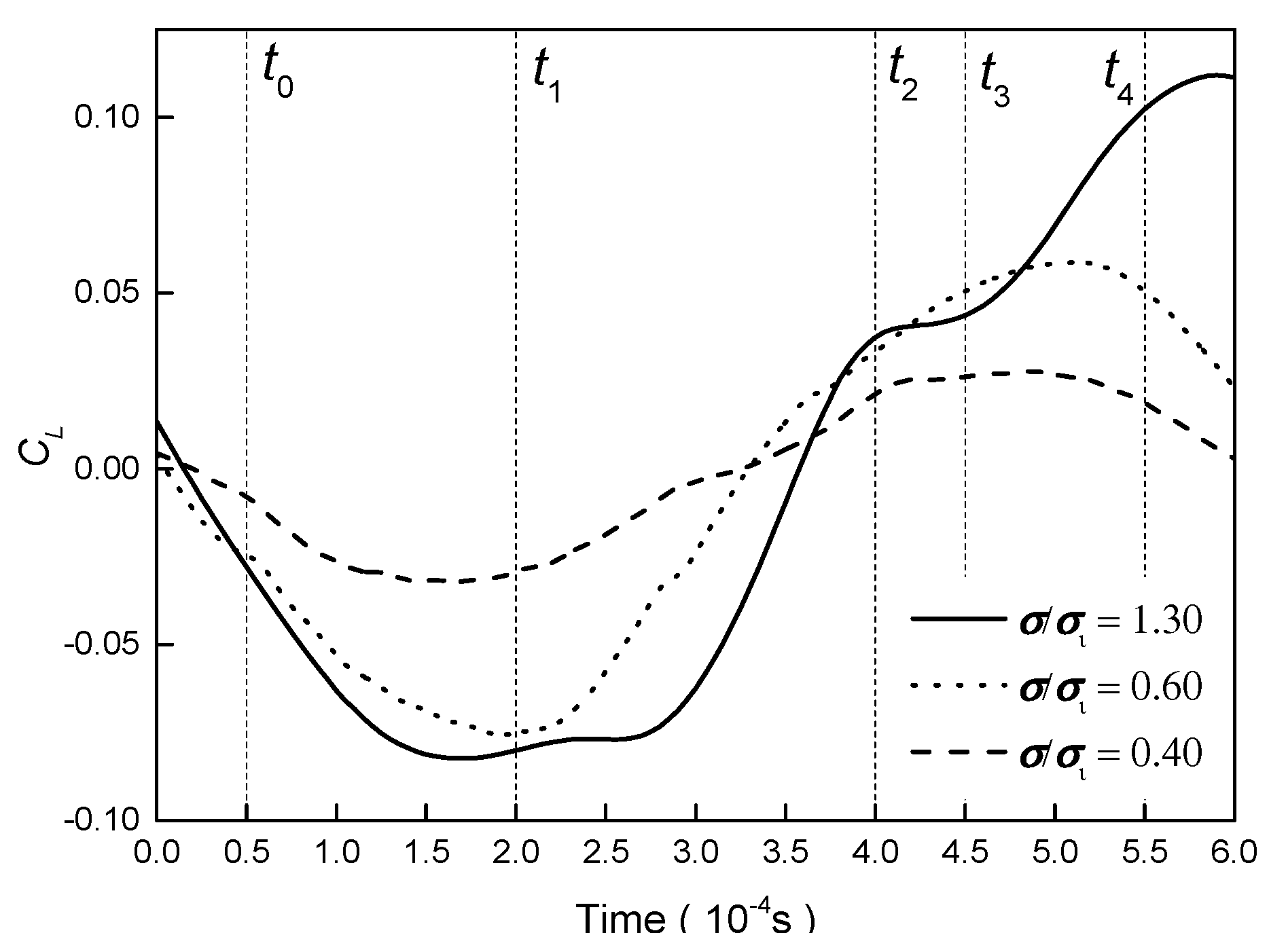
Figure 8 shows the time history of CL over 6 × 10⁻⁴ s for the different cavitation conditions. Five typical instants of time were marked (from t0 to t4) to compare the vortex shedding process among the three flow conditions. For each instance, the instantaneous Eulerian Q criterion was derived from a snapshot of the velocity field and its gradient. Moreover, the contour of the backward FTLE scalar was also calculated considering as the initial time the one corresponding to each of the selected time instants. It should be mentioned here that the finite integration time, T, was chosen equal to −0.0015 s, which corresponds to almost two periods of the vortex shedding process. In fact, no significant differences are found among the results if larger integration times are considered.
In Figure 9, both the evolution of the Eulerian Q criterion on the instantaneous velocity field and the backward FTLE scalar levels display the alternating vortex shedding cycle behind the trailing edge at free cavitation conditions. At instant t0, both the closer upper vortex to the trailing edge, marked with letter “A”, and the closer lower vortex, marked with letter “B”, are observed immediately behind the hydrofoil at the vortex formation region. At this time, vortex A has a larger size than vortex B. From t0 to t1, vortex B continues its growth and induces enough velocity to the wake flow so that the link between the upper boundary shear layer and vortex A is cut off. Thus, vortex A reaches its maximum size at instant t1. Then, the upper vortex A is shed from the vortex formation area, which corresponds to the minimum value of the lift coefficient. From t1 to t4, a new upper vortex appears, marked with the letter “C”, and it grows as it is fed by the upper boundary shear layer. When it reaches sufficient size to cut off the previous lower vortex B, the process already described for vortex A is repeated by vortex C. In general, all the shed vortices take a circular shape and the two rows of vortices are clearly separated in the transverse direction. All these observations of the vortex shedding evolution are in agreement with the results for a bluff body obtained by Wang et al. [60].
As cavitation occurs, the instantaneous contour of the vapor volume fraction, the instantaneous Eulerian Q criterion and the contours of the backward FTLE scalars are plotted in Figure 10 and Figure 11 for two degrees of cavitation.
At σ/σi = 0.60, the pressure inside the vortex center decreases to the vapor pressure, pv, and the vortices cavitate at their cores, as it can be seen in Figure 10a where the graphs show the evolution of the vapor volume fraction. Firstly, the upper cavitating vortex A is being formed at instant t0. Then, vortex A is stretched and reaches its maximum size at instant t1 when CL is minimum. From t1 to t2, the vapor also fills a long filament that connects the cavitating upper vortex A with the trailing edge region. After that moment, vortex A is completely detached from the trailing edge and the lower cavitating vortex B is still attached to the trailing edge and begins to be stretched. Further, a new upper cavitating vortex C begins to be formed. From t2 to t3, vortex B continues to be stretched and its size keeps increasing. Finally and just before instant t4, vortex B is cut off by vortex C and completely shed from the trailing edge area.
At σ/σi = 0.40, the instantaneous evolution of the vapor volume fraction presented in Figure 11a permits observing that the cavitating vortices are more stretched than at σ/σi = 0.60. From t1 to t2, it is observed that the upper cavitating vortex A is connected to the upper and lower cavitating vortices C and B, respectively, by a thin cavitation filament. Then, at t3, the lower cavitating vortex B separates from the upper vortex C, and vortex A is completely shed downstream. At t4, it can be seen how two vortices coexist in contact with the hydrofoil trailing edge which corresponds to vortex C and to the rear part of vortex B that occupies the very near wake and provokes the boundary layers coming from the extrados and the intrados to require a longer distance to create shed new vortices.
In Figure 10b or Figure 11b, the instantaneous contour plots of the Eulerian Q criterion show the evolution of the vortex shedding and the simultaneous velocity field under cavitation conditions. Compared with the free cavitation condition presented in Figure 9a, it is observed that the shedding vortex pattern and shapes of the vortices near the trailing edge are significantly affected by the occurrence of cavitation. For example, at instant t1, the dimensions of vortex B tend to increase as the cavitation number decreases. Moreover, the vortices are elongated in the main flow direction and they cannot be entirely cut off by the opposite vortex. Consequently, their rear part remains attached to the blunt trailing edge instead of being shed with the front part.
In Figure 10c or Figure 11c, the instantaneous contour plots of the backward FTLE scalar show the evolution of the vortex shedding from the Lagrangian viewpoint. The obtained results are in agreement with the previous observation and thus confirm that the morphology and shape of the vortices continue to be affected by the increasing level of cavitation as well as their formation length.
In summary, at the free cavitation condition, the two rows of vortices are well separated in the transverse direction and each vortex depicts a well-defined circular shape. However, under cavitation conditions, the tranverse distance between the two rows is significantly reduced and the vortices change their shape towards an elliptical one mainly elongated in the transverse direction. As cavitation increases, the sizes of the vortices decrease and they are almost in line with the horizontal axis of the hydrofoil. Therefore, all the results seem to indicate that the effective height of the near wake formation region is significantly reduced which explains the fact that the shedding frequency is increased if the Strouhal number is assumed to be invariant.
4. Conclusions
The characteristics of the cavitating wake flow of a 2D NACA0009 with a blunt trailing edge have been numerically investigated and compared with the free cavitation conditions by means of the LES WALE turbulence model and the Zwart cavitation model. The numerical setup has been validated in comparison with experimental observations. To understand the effects of cavitation on the vortex shedding process, two vortex identification criteria based on the Eulerian and Lagrangian frames of reference have been applied to the unsteady flow velocity field. The following conclusions have been obtained:
- Vortices shape: it has been observed that the circular shape of the vortices changes to an elliptical one as they are stretched in the streamwise direction with the development of cavitation.
- Vortices transverse separation: it has been observed that the transverse separation between the upper and lower rows of vortices is reduced with the development of cavitation.
- Vortex formation length: it has been numerically found that the vortex formation length increases by around 83% with the development and growth of cavitation in the wake flow in comparison with the free cavitation condition when the cavitation number is reduced to 40% of the incipient cavitation number.
- Vortex shedding frequency: it has been numerically found that the vortex shedding frequency increases by 14% with the development and growth of cavitation in the wake flow in comparison with the free cavitation condition when the cavitation number is reduced to 40% of the incipient cavitation number.
Author Contributions
Conceptualization, J.C. and X.E.; methodology, J.C.; validation, J.C. and L.G.; writing—original draft preparation, J.C.; writing—review and editing, J.C, L.G. and X.E.; supervision, X.E. All authors have read and agreed to the published version of the manuscript.
Funding
The present research work was financially supported China Scholarship Council (No 201808320237).
Conflicts of Interest
The authors declare no conflict of interest.
References
- Arndt, R.E. Cavitation in fluid machinery and hydraulic structures. Annu. Rev. Fluid Mech. 1981, 13, 273–326. [Google Scholar] [CrossRef]
- Franc, J.P.; Michel, J.M. Fundamentals of Cavitation; Springer Science & Business Media: Berlin, Germany, 2006; pp. 1–13, 247–262. [Google Scholar]
- Arndt, R.E. Cavitation in vortical flows. Annu. Rev. Fluid Mech. 2002, 34, 143–175. [Google Scholar] [CrossRef]
- Belahadji, B.; Franc, J.P.; Michel, J.M. Cavitation in the rotational structures of a turbulent wake. J. Fluid Mech. 1995, 287, 383–403. [Google Scholar] [CrossRef]
- Gerrard, J.H. The mechanics of the formation region of vortices behind bluff bodies. J. Fluid Mech. 1966, 25, 401–413. [Google Scholar] [CrossRef]
- Williamson, C.H. Vortex dynamics in the cylinder wake. Annu. Rev. Fluid Mech. 1996, 28, 477–539. [Google Scholar] [CrossRef]
- Kim, J.; Choi, H. Distributed forcing of flow over a circular cylinder. Phys. Fluids 2005, 17, 103–116. [Google Scholar] [CrossRef]
- Roshko, A. On the Drag and Shedding Frequency of Two-Dimensional Bluff Bodies; National Aeronautics and Space Administration: Washington, DC, USA, 1954.
- Farhadi, M.; Sedighi, K.; Korayem, A.M. Effect of wall proximity on forced convection in a plane channel with a built-in triangular cylinder. Int. J. Therm. Sci. 2010, 49, 1010–1018. [Google Scholar] [CrossRef]
- Varga, J.; Sebestyen, G.Y. Determination of the frequencies of wakes shedding from circular cylinders. Acta Tech. Acad. Sci. Hung. 1966, 53, 91–108. [Google Scholar]
- Syamala Rao, B.C.; Chandrasekhara, D.V. Some characteristics of cavity flow past cylindrical inducers in a Venturi. J. Fluids Eng. 1976, 98, 461–466. [Google Scholar] [CrossRef]
- Ramamurthy, A.S.; Balachandar, R. Characteristics of constrained cavitating bluff body wakes. J. Eng. Mech. 1991, 117, 513–531. [Google Scholar] [CrossRef]
- Gnanaskandan, A.; Mahesh, K. Numerical investigation of near-wake characteristics of cavitating flow over a circular cylinder. J. Fluid Mech. 2016, 790, 453–491. [Google Scholar] [CrossRef] [Green Version]
- Young, J.O.; Holl, J.W. Effects of cavitation on periodic wakes behind symmetric wedges. J. Fluids Eng. 1966, 88, 163–176. [Google Scholar] [CrossRef]
- Ramamurthy, A.S.; Bhaskaran, P. Constrained flow past cavitating bluff bodies. J. Fluids Eng. 1977, 99, 717–726. [Google Scholar] [CrossRef]
- Deijlen, L.; Bhatt, A.; Ganesh, H.; Wu, J.; Ceccio, S. Cavitation Dynamics in Wakes Behind Bluff Bodies. Bull. Am. Phys. Soc. 2018, 63. [Google Scholar] [CrossRef] [Green Version]
- Gnanaskandan, A.; Mahesh, K. Large eddy simulation of the transition from sheet to cloud cavitation over a wedge. Int. J. Multiph. Flow 2016, 83, 86–102. [Google Scholar] [CrossRef] [Green Version]
- Park, S.; Lee, H.; Choi, H.K.; Rhee, S.H.; Choe, Y.; Kim, H.; Kim, C.; Kim, J.H.; Ahn, B.K.; Kim, H.T. Cavity Dynamics Behind a 2-D Wedge Analyzed by Incompressible and Compressible Flow Solvers. In Proceedings of the 9th International Symposium on Cavitation, Lausanne, Switzerland, 6–10 December 2015. [Google Scholar]
- Balachandar, R.; Ramamurthy, A.S. Pressure distribution in cavitating circular cylinder wakes. J. Eng. Mech. 1999, 125, 356–358. [Google Scholar] [CrossRef]
- Ausoni, P. Turbulent Vortex Shedding from a Blunt Trailing Edge Hydrofoil. Ph.D. Thesis, EPFL, Lausanne, Switzerland, 2009. [Google Scholar]
- Kumar, P.; Chatterjee, D.; Bakshi, S. Experimental investigation of cavitating structures in the near wake of a cylinder. Int. J. Multiph. Flow 2017, 89, 207–217. [Google Scholar] [CrossRef]
- Lee, S.J.; Lee, J.H.; Suh, J.C. Further validation of the hybrid particle-mesh method for vortex shedding flow simulations. Int. J. Nav. Archit. Ocean Eng. 2015, 7, 1034–1043. [Google Scholar] [CrossRef] [Green Version]
- Chen, J.; Li, Y.J.; Liu, Z.Q. Large eddy simulation of boundary layer transition flow around NACA0009 blunt trailing edge hydrofoil at high Reynolds number. In Proceedings of the 29th IAHR’s Symposium on Hydraulic Machinery and Systems, Kyoto, Japan, 16–21 September 2018. [Google Scholar]
- Kim, J.H.; Jeong, S.W.; Ahn, B.K. Numerical and experimental study on unsteady behavior of cavitating flow around a two-dimensional wedge-shaped body. J. Mar. Sci. Technol. 2019, 24, 1256–1264. [Google Scholar] [CrossRef]
- Cheng, H.; Long, X.; Ji, B.; Peng, X.; Farhat, M. A new Euler-Lagrangian cavitation model for tip-vortex cavitation with the effect of non-condensable gas. Int. J. Multiph. Flow 2020, 11, 103–141. [Google Scholar]
- Cheng, H.Y.; Bai, X.R.; Long, X.P.; Ji, B.; Peng, X.X.; Farhat, M. Large eddy simulation of the tip-leakage cavitating flow with an insight on how cavitation influences vorticity and turbulence. Appl. Math. Model. 2020, 1, 788–809. [Google Scholar] [CrossRef]
- Arabnejad, M.H.; Amini, A.; Farhat, M.; Bensow, R.E. Numerical and experimental investigation of shedding mechanisms from leading-edge cavitation. Int. J. Multiph. Flow 2019, 1, 123–143. [Google Scholar] [CrossRef]
- Decaix, J.; Balarac, G.; Dreyer, M.; Farhat, M.; Münch, C. RANS and LES computations of the tip-leakage vortex for different gap widths. J. Turbul. 2015, 16, 309–341. [Google Scholar] [CrossRef]
- Trummler, T.; Schmidt, S.J.; Adams, N.A. Investigation of condensation shocks and re-entrant jet dynamics in a cavitating nozzle flow by Large-Eddy Simulation. Int. J. Multiph. Flow 2020, 1, 215–241. [Google Scholar] [CrossRef] [Green Version]
- Budich, B.; Schmidt, S.J.; Adams, N.A. Numerical simulation and analysis of condensation shocks in cavitating flow. J. Fluid Mech. 2018, 10, 759–791. [Google Scholar] [CrossRef]
- Chen, Z.; Adams, N.A. Mode interactions of a high-subsonic deep cavity. Phys. Fluids 2017, 29, 56–82. [Google Scholar] [CrossRef]
- Ghahramani, E.; Jahangir, S.; Neuhauser, M.; Bourgeois, S.; Poelma, C.; Bensow, R.E. Experimental and numerical study of cavitating flow around a surface mounted semi-circular cylinder. Int. J. Multiph. Flow 2020, 9, 191–223. [Google Scholar] [CrossRef]
- Asnaghi, A.; Svennberg, U.; Bensow, R.E. Large Eddy Simulations of cavitating tip vortex flows. Ocean. Eng. 2020, 195, 106–133. [Google Scholar] [CrossRef]
- Asnaghi, A.; Feymark, A.; Bensow, R.E. Numerical investigation of the impact of computational resolution on shedding cavity structures. Int. J. Multiph. Flow 2018, 10, 33–50. [Google Scholar] [CrossRef]
- Schenke, S.; van Terwisga, T. Simulating compressibility in cavitating flows with an incompressible mass transfer flow solver. In Proceedings of the Fifth International Symposium on Marine Propulsors, Espoo, Finland, 12–15 June 2017. [Google Scholar]
- Brunhart, M.; Soteriou, C.; Gavaises, M.; Karathanassis, I.; Koukouvinis, P.; Jahangir, S.; Poelma, C. Investigation of cavitation and vapor shedding mechanisms in a Venturi nozzle. Phys. Fluids. 2020, 32, 83–106. [Google Scholar] [CrossRef]
- Cristofaro, M.; Edelbauer, W.; Koukouvinis, P.; Gavaises, M. A numerical study on the effect of cavitation erosion in a diesel injector. Appl. Math. Model. 2020, 2, 200–216. [Google Scholar] [CrossRef]
- Mithun, M.G.; Koukouvinis, P.; Gavaises, M. Numerical simulation of cavitation and atomization using a fully compressible three-phase model. Phys. Rev. Fluids. 2018, 3, 64–87. [Google Scholar] [CrossRef] [Green Version]
- Epps, B. Review of vortex identification methods. In Proceedings of the 55th AIAA Aerospace Sciences Meeting, Grapevine, TX, USA, 9–13 January 2017. [Google Scholar]
- Saffman, P.G. Vortex Dynamics; Cambridge University Press: Cambridge, UK, 1992. [Google Scholar]
- Hunt, J.C.; Wray, A.A.; Moin, P. Eddies, streams, and convergence zones in turbulent flows. In Proceedings of the 1988 Summer Program, Standford, CA, USA, 1 December 1988. [Google Scholar]
- Chong, M.S.; Perry, A.E.; Cantwell, B.J. A general classification of three-dimensional flow fields. Phys. Fluids A Fluid Dyn. 1990, 2, 765–777. [Google Scholar] [CrossRef]
- Zhang, Y.; Liu, K.; Xian, H.; Du, X. A review of methods for vortex identification in hydroturbines. Renew. Sustain. Energy Rev. 2018, 81, 1269–1285. [Google Scholar] [CrossRef]
- Brown, G.L.; Roshko, A. On density effects and large structure in turbulent mixing layers. J. Fluid Mech. 1974, 64, 775–816. [Google Scholar] [CrossRef] [Green Version]
- Robinson, S.K. Coherent motions in the turbulent boundary layer. Annu. Rev. Fluid Mech. 1991, 23, 601–639. [Google Scholar] [CrossRef]
- Haller, G. Finding finite-time invariant manifolds in two-dimensional velocity fields. Chaos Interdiscip. J. Nonlinear Sci. 2000, 10, 99–108. [Google Scholar] [CrossRef]
- Haller, G. Distinguished material surfaces and coherent structures in three-dimensional fluid flows. Phys. D Nonlinear Phenom. 2001, 149, 248–277. [Google Scholar] [CrossRef] [Green Version]
- Shadden, S.C.; Dabiri, J.O.; Marsden, J.E. Lagrangian analysis of fluid transport in empirical vortex ring flows. Phys. Fluids 2006, 18, 047105. [Google Scholar] [CrossRef] [Green Version]
- O’Farrell, C.; Dabiri, J.O. A Lagrangian approach to identifying vortex pinch-off. Chaos Interdiscip. J. Nonlinear Sci. 2010, 20, 017513. [Google Scholar] [CrossRef] [Green Version]
- O’Farrell, C.; Dabiri, J.O. Pinch-off of non-axisymmetric vortex rings. J. Fluid Mech. 2014, 740, 61–96. [Google Scholar] [CrossRef] [Green Version]
- Green, M.A.; Rowley, C.W.; Smits, A.J. The unsteady three-dimensional wake produced by a trapezoidal pitching panel. J. Fluid Mech. 2011, 685, 117–145. [Google Scholar] [CrossRef] [Green Version]
- Rockwood, M.P.; Taira, K.; Green, M.A. Detecting vortex formation and shedding in cylinder wakes using Lagrangian coherent structures. AIAA J. 2017, 55, 15–23. [Google Scholar] [CrossRef]
- Eldredge, J.D.; Chong, K. Fluid transport and coherent structures of translating and flapping wings. Chaos Interdiscip. J. Nonlinear Sci. 2010, 20, 017509. [Google Scholar] [CrossRef] [PubMed]
- Rukes, L.; Sieber, M.; Oliver Pashereit, C.; Oberleithner, K. Methods for the extraction and analysis of the global mode in swirling jets undergoing vortex breakdown. J. Eng. Gas Turbines Power 2017, 139, 022604. [Google Scholar] [CrossRef]
- Sadlo, F.; Peikert, R. Visualizing lagrangian coherent structures and comparison to vector field topology. In Topology-Based Methods in Visualization II; Springer: Berlin/Heidelberg, Germany, 2009. [Google Scholar]
- Beron-Vera, F.J.; Olascoaga, M.J.; Goni, G.J. Oceanic mesoscale eddies as revealed by Lagrangian coherent structures. Geophys. Res. Lett. 2008, 35. [CrossRef]
- Du Toit, P.C.; Marsden, J.E. Horseshoes in hurricanes. J. Fixed Point Theory Appl. 2010, 7, 351–384. [Google Scholar] [CrossRef]
- Haller, G. Lagrangian coherent structures. Annu. Rev. Fluid Mech. 2015, 47, 137–162. [Google Scholar] [CrossRef] [Green Version]
- Tseng, C.C.; Liu, P.B. Dynamic behaviors of the turbulent cavitating flows based on the Eulerian and Lagrangian viewpoints. Int. J. Heat Mass Transf. 2016, 102, 479–500. [Google Scholar] [CrossRef]
- Wang, Z.; Huang, B.; Zhang, M.; Wang, G.; Ji, B. Numerical investigation of ventilated cavitating vortex shedding over a bluff body. Ocean Eng. 2018, 159, 129–138. [Google Scholar] [CrossRef]
- Zwart, P.J.; Gerber, G.; Belamri, T. A two-phase flow model for prediction cavitation dynamics. In Proceedings of the 5th International Conference Multiphase Flow (ICMF 2004), Yokohama, Japan, 30 May–4 June 2004. [Google Scholar]
- Nicoud, F.; Ducros, F. Subgrid-scale stress modelling based on the square of the velocity gradient tensor. Flow Turbul. Combust. 1999, 62, 183–200. [Google Scholar] [CrossRef]
- Smagorinsky, J. General circulation experiments with the primitive equations: I. The basic experiment. Mon. Weather. Rev. 1963, 91, 99–164. [Google Scholar] [CrossRef]
- Ait Bouziad, Y. Physical Modelling of Leading Edge Cavitation: Computational Methodologies and Application to Hydraulic Machinery. Ph.D. Thesis, EPFL, Lausanne, Switzerland, 2005. [Google Scholar]
- Griffin, O.M. A note on bluff body vortex formation. J. Fluid Mech. 1995, 284, 217–224. [Google Scholar] [CrossRef]
Figure 1.
Computational domain with dimensions (a) and mesh topology close to the hydrofoil surface and near wake region (b).
Figure 1.
Computational domain with dimensions (a) and mesh topology close to the hydrofoil surface and near wake region (b).

Figure 2.
Contour plot of the ratio between the mesh resolution, Δ, and the Taylor scales.

Figure 3.
Comparison of: (a) numerical mean pressure coefficient, Cp, with the vortex panel method as a function of the dimensionless position, x/L; (b) numerical mean normalized horizontal and vertical velocities, ux,mean/Vinlet and uy,mean/Vinlet respectively, with experimental results at different vertical dimensionless positions, y/tmax.

Figure 4.
Time history of the lift and drag coefficients, CL and CD, at: (a) free cavitation conditions (σ/σi = 1.3); (b) cavitation conditions (σ/σi = 0.6); and (c) cavitation conditions (σ/σi = 0.4).
Figure 4.
Time history of the lift and drag coefficients, CL and CD, at: (a) free cavitation conditions (σ/σi = 1.3); (b) cavitation conditions (σ/σi = 0.6); and (c) cavitation conditions (σ/σi = 0.4).

Figure 5.
Spectra of the time evolution of the lift coefficient at free cavitation conditions (σ/σi = 1.3) and at two cavitation conditions (σ/σi = 0.6 and 0.4).
Figure 5.
Spectra of the time evolution of the lift coefficient at free cavitation conditions (σ/σi = 1.3) and at two cavitation conditions (σ/σi = 0.6 and 0.4).

Figure 6.
Comparison of Strouhal, St, estimates between the numerical simulations and the experimental measurements at free cavitation conditions and at cavitation conditions.
Figure 6.
Comparison of Strouhal, St, estimates between the numerical simulations and the experimental measurements at free cavitation conditions and at cavitation conditions.

Figure 7.
Root mean square value of the fluctuating velocity normalized by the inlet flow velocity, , at different distances, x, from the trailing edge of the hydrofoil along a horizontal line for free cavitation and cavitation conditions.
Figure 7.
Root mean square value of the fluctuating velocity normalized by the inlet flow velocity, , at different distances, x, from the trailing edge of the hydrofoil along a horizontal line for free cavitation and cavitation conditions.

Figure 8.
Comparison of lift coefficient, CL, evolutions during less than one shedding period at different cavitation conditions.
Figure 8.
Comparison of lift coefficient, CL, evolutions during less than one shedding period at different cavitation conditions.

Figure 9.
Plot for free cavitation conditions (σ/σi = 1.3) at five correlative instants of time from top to bottom of: (a) the instantaneous Eulerian Q criterion superposed to the instantaneous velocity; (b) the backward finite-time Lyapunov exponent (FTLE).
Figure 9.
Plot for free cavitation conditions (σ/σi = 1.3) at five correlative instants of time from top to bottom of: (a) the instantaneous Eulerian Q criterion superposed to the instantaneous velocity; (b) the backward finite-time Lyapunov exponent (FTLE).


Figure 10.
Plot for cavitation conditions (σ/σi = 0.6) at five correlative instants of time from top to bottom of: (a) vapor volume fraction distribution; (b) the instantaneous Eulerian Q criterion superposed to the instantaneous velocity; and (c) the backward finite-time Lyapunov exponent (FTLE).
Figure 10.
Plot for cavitation conditions (σ/σi = 0.6) at five correlative instants of time from top to bottom of: (a) vapor volume fraction distribution; (b) the instantaneous Eulerian Q criterion superposed to the instantaneous velocity; and (c) the backward finite-time Lyapunov exponent (FTLE).

Figure 11.
Plot for cavitation conditions (σ/σi = 0.4) at five correlative instants of time from top to bottom of: (a) vapor volume fraction distribution; (b) the instantaneous Eulerian Q criterion superposed to the instantaneous velocity; and (c) the backward finite-time Lyapunov exponent (FTLE).
Figure 11.
Plot for cavitation conditions (σ/σi = 0.4) at five correlative instants of time from top to bottom of: (a) vapor volume fraction distribution; (b) the instantaneous Eulerian Q criterion superposed to the instantaneous velocity; and (c) the backward finite-time Lyapunov exponent (FTLE).


Table 1.
Details of the checked meshes and results obtained for the mesh independency study.
| Name | Number of Elements | Max y+ [–] | Resolution in Near Wake [mm] | Outlet Boundary Location | Shedding Frequency [Hz] | St [–] | Deviation [%] |
|---|---|---|---|---|---|---|---|
| MC | 29525 | 3.5 | 0.6 | 3C | 1550 | 0.250 | 10.7 |
| MM | 49420 | 2.8 | 0.4 | 3C | 1500 | 0.242 | 7.1 |
| MF_1 | 71200 | 2.8 | 0.2 | 3C | 1450 | 0.233 | 3.6 |
| MF_2 | 313790 | 0.38 | 0.2 | 6C | 1450 | 0.233 | 3.6 |
Publisher’s Note: MDPI stays neutral with regard to jurisdictional claims in published maps and institutional affiliations. |
© 2020 by the authors. Licensee MDPI, Basel, Switzerland. This article is an open access article distributed under the terms and conditions of the Creative Commons Attribution (CC BY) license (http://creativecommons.org/licenses/by/4.0/).
Share and Cite
MDPI and ACS Style
Chen, J.; Geng, L.; Escaler, X. Numerical Investigation of the Cavitation Effects on the Vortex Shedding from a Hydrofoil with Blunt Trailing Edge. Fluids 2020, 5, 218. https://doi.org/10.3390/fluids5040218
AMA Style
Chen J, Geng L, Escaler X. Numerical Investigation of the Cavitation Effects on the Vortex Shedding from a Hydrofoil with Blunt Trailing Edge. Fluids. 2020; 5(4):218. https://doi.org/10.3390/fluids5040218
Chicago/Turabian StyleChen, Jian, Linlin Geng, and Xavier Escaler. 2020. "Numerical Investigation of the Cavitation Effects on the Vortex Shedding from a Hydrofoil with Blunt Trailing Edge" Fluids 5, no. 4: 218. https://doi.org/10.3390/fluids5040218