Hydrodynamic Responses of a 6 MW Spar-Type Floating Offshore Wind Turbine in Regular Waves and Uniform Current


1
College of Shipbuilding Engineering, Harbin Engineering University, Harbin 150001, China
2
Technology Centre for Offshore and Marine, Singapore (TCOMS), Singapore 118411, Singapore
3
School of Naval Architecture, Ocean & Civil Engineering, Shanghai Jiao Tong University, Shanghai 200240, China
4
Department of Mechanical Engineering, Technical University of Denmark, 2800 Lyngby, Denmark
*
Author to whom correspondence should be addressed.
Fluids 2020, 5(4), 187; https://doi.org/10.3390/fluids5040187
Submission received: 16 September 2020
/
Revised: 15 October 2020
/
Accepted: 17 October 2020
/
Published: 21 October 2020
(This article belongs to the Special Issue Wind and Wave Renewable Energy Systems)
Abstract
:In order to improve the understanding of hydrodynamic performances of spar-type Floating Offshore Wind Turbines (FOWTs), in particular the effect of wave-current-structure interaction, a moored 6MW spar-type FOWT in regular waves and uniform current is considered. The wind loads are not considered at this stage. We apply the potential-flow theory and perturbation method to solve the weakly-nonlinear problem up to the second order. Unlike the conventional formulations in the inertial frame of reference, which involve higher derivatives on the body surface, the present method based on the perturbation method in the non-inertial body-fixed coordinate system can potentially avoid theoretical inconsistency at sharp edges and associated numerical difficulties. A cubic Boundary Element Method (BEM) is employed to solve the resulting boundary-value problems (BVPs) in the time domain. The convective terms in the free-surface conditions are dealt with using a newly developed conditionally stable explicit scheme, which is an approximation of the implicit Crank–Nicolson scheme. The numerical model is firstly verified against three reference cases, where benchmark results are available, showing excellent agreement. Numerical results are also compared with a recent model test, with a fairly good agreement though differences are witnessed. Drag loads based on Morison’s equation and relative velocities are also applied to quantify the influence of the viscous loads. To account for nonlinear restoring forces from the mooring system, a catenary line model is implemented and coupled with the time-domain hydrodynamic solver. For the considered spar-type FOWT in regular-wave and current conditions, the current has non-negligible effects on the motions at low frequencies, and a strong influence on the mean wave-drift forces. The second-order sum-frequency responses are found to be negligibly small compared with their corresponding linear components. The viscous drag loads do not show a strong influence on the motions responses, while their contribution to the wave-drift forces being notable, which increases with increasing wave steepness.
1. Introduction
As abundant reserves of renewable wind energy resources are available at offshore sites where water depths are not small, different concepts of Floating Offshore Wind Turbines (FOWTs) have been proposed as cost-efficient alternatives to bottom-mounted wind turbines that are being commonly used in the shallow water regions. Significant progress has been made in the preliminary design and verification of FOWTs in recent years [1,2,3,4,5,6,7]. Inspired by the experiences and practice of offshore engineering, different floating support platforms have been proposed for the offshore-wind industry, including: the semisubmersibles, Tension Leg Platforms (TLPs), and spar buoys. Among others, FOWTs that have been widely studied experimentally or theoretically include OC4-DeepCwind semisubmersible platform [3,8,9], UMaine TLP [10,11], OC3-Hywind spar buoy, [5,12,13,14,15], etc.
FOWT is a complex coupled system involving aerodynamics, hydrodynamics, structural elasticity, and the control system. For the hydrodynamic loads, experiences from offshore engineering show that the 2nd-order hydrodynamic effects usually play an important role in analyzing the dynamic responses of marine structures [16,17]. The 2nd-order wave loads consist of an average component, i.e., mean-drift force, as well as sum-frequency (SF) and difference-frequency (DF) loads. The latter two components may excite the resonant responses of the structures since the oscillatory frequencies of these 2nd-order components may be close to certain natural frequencies of the structures, even though the natural frequencies are intentionally designed to be away from the wave frequencies where significant wave energy exists. Examples are slow-drift motions of compliant floating structures excited by the DF wave loads, and springing of TLPs excited by the SF wave loads. The significance of 2nd-order SF and DF wave loads on the dynamic response of FOWTs has been reported and discussed in the literature for spar-type FOWTs [5,18,19], semisubmersible FOWTs [20,21,22], and TLP FOWTs [18,23,24,25].
Even though the spar-type FOWT concept has its own limitations, for instance, it cannot be used at small water depths due to its deep draft, it has excellent stability and hydrodynamic properties. In general, a spar-type FOWT has smaller heave motions in contrast to semi-submersibles owing to their deep draft and reduced vertical wave excitation forces. Compared with TLPs, it has preferable stability due to a low gravity center.
The effects of 2nd-order wave excitation loads on the dynamic responses of spar-type FOWTs have been investigated in previous studies. Close to the natural frequencies of the OC3-Spar FOWT, Browning et al. [5] noticed that the second harmonics of the dynamic response observed in model tests are larger than the numerical results of a FAST model [26], which only includes the linear wave loads through the hydrodynamic coefficients calculated in its HydroDyn module. FAST is one of the commonly-used time-domain simulation tools for coupled dynamic analysis of wind turbines, developed by NREL. Roald et al. [18] used WAMIT to calculate the linear and 2nd-order hydrodynamic coefficients, and FAST to simulate the dynamic responses of OC3-Hywind Spar in the time domain. Both Newman’s approximation and the full Quadratic Transfer function (QTF) method have been applied. It was found that resonant motions are excited by the 2nd-order wave loads, especially for the heave motion even though the 2nd-order excitation loads are significantly small. From a practical point of view, it is convenient to use such a model in design of FOWTs, where the 2nd-order wave-load effects cannot be neglected [22,27]. The time-domain model in FAST is based on a Cummins-type of equations used for retardation functions so that the memory effects are also included. In addition, extra damping (e.g., viscous damping) or restoring forces from, for instance, the mooring system, can be included through the time-domain motion equations. However, the limitation of this type of hybrid method, combining a frequency-domain code (e.g., WAMIT or similar) and a time-domain tool like FAST, is obvious as well. It is not straightforward to include the viscous effects in a frequency-domain analysis, in particular when the calculated hydrodynamic coefficients will be used as inputs to the time-domain models to simulate the dynamic responses of FOWTs in irregular waves. A frequency-domain model without appropriate modeling of viscous effects may produce non-physically large resonant motions, and thus yields wrong QTFs for the 2nd-order wave loads. If an equivalent linear damping is introduced in the frequency-domain analysis to represent the nonlinear damping through e.g., the drag forces, seastate-dependent damping should be considered, using for instance stochastic linearization [28,29,30], which, however, also needs careful calibration towards the models tests.
Solving the hydrodynamic boundary-value problems (BVPs) directly in the time domain offers the possibility to simultaneously compute the potential-flow induced wave loads and the viscous loads through empirical formulae, e.g., drag term in the Morison-type of equations, without having to make equivalent linearization. Such direct time-domain models have already been developed up to the 2nd order with success. Examples are Shao [31] using a cubic BEM based on piece-wise shape functions, Bai and Teng [32] using a spline-based BEM and Duan et al. [33] using a Taylor-expanded BEM.
The majority of direct time-domain 2nd-order models reported in the literature ignore the forward speed or current effects. However, the current speeds at the offshore sites may not be negligible, in particular for FOWT applications where the characteristic cross-section dimensions are small. As it will be shown later, the radius-based Froude number may reach 0.2 for the considered 6MW spar-type FOWT foundation using a typical current speed of around 1.4 m/s. Therefore, it is of great interest to look into the wave–current–structure interaction and investigate the current effects.
To the best of the authors’ knowledge in the available literature, there are very few attempts to consistently take account of the forward speed or current effects in the 2nd-order models. Based on body-fixed coordinate system, an alternative formulation of the seakeeping problem has been developed by Shao and Faltinsen [34,35,36] up to the 2nd order with the consideration of forward speed. This formulation does not involve any higher derivatives on the body surface. It also mathematically avoids the inconsistencies that a traditional formulation in an earth-fixed coordinate system has. To overcome the difficulties of the traditional formulation when the expansion parameter is not small, Teng et al. [37] proposed a twice-expansion method to study the wave–structure interaction problems, allowing for large horizontal motions of the structures.
In the present study, the complete 2nd-order time-domain model of Shao and Faltinsen [34,35,36] is extended to study moored floating structures in waves and current. To the best of our knowledge, it is the first time in the literature that a complete and consistent 2nd-order model is used for FOWT applications. Furthermore, a conditionally stable explicit time-integration scheme, recently proposed by Shao [38] for advection equations, is employed to stabilize the solution and reduce the computational costs. The scheme is obtained through an approximation of the unconditionally stable implicit Crank–Nicolson scheme. To avoid drifting of the structures, a catenary line model is implemented and coupled with the time-domain hydrodynamic solver.
Theoretically, the present model is more advanced than the existing state-of-the-art open-source or commercial hydrodynamic solvers based on perturbation schemes, for example, the WASIM solver from DNVGL SESAM software package or others alike. WASIM is a popularly used commercial time-domain seakeeping code with forward speed effect. However, it does not solve a 2nd-order wave–structure interaction problem. In other words, it does not provide complete 2nd-order SF and DF wave loads. Other hybrid time-domain solvers, e.g., the SIMO solver in SESAM, which takes frequency-domain linear and 2nd-order transfer functions as inputs, do not however consistently consider the wave–current–structure interaction. On the contrary, the present model is a complete 2nd-order wave–structure model, consistently taking into account the current or forward speed effect. Since we use a potential-flow approach, the drag loads can only be approximated empirically through e.g., the drag term in Morison’s equation, as it will be presented later in Section 3.3. In principle, a wind-load model based on e.g., blade element method, could also be included, which will be considered in our future studies.
The hydrodynamic performance of a 6 MW spar-type FOWT in waves and current is studied after the verification of the numerical model. The rest of the paper is organized as follows: Section 2 presents the theoretical formulation, followed by the description of the numerical model in Section 3. The numerical model will be verified in Section 4. In Section 5, we present the numerical studies on the 6 MW spar-type FOWT. Finally, conclusions will be summarized in Section 6 together with future perspectives.
2. Theoretical Description
2.1. Definition and Governing Equation
It is assumed that the fluid is inviscid and incompressible, and flow is irrotational so that a velocity potential exists. Then, the motion of fluid particle can be described by the velocity potential, which satisfies the governing equation, i.e., the Laplace equation:
To describe the BVPs in the presence of a steady forward speed or a uniform current in this section, three right-handed Cartesian coordinate systems are defined, as shown in Figure 1. The three reference frames consist of two inertial coordinate systems: an Earth-fixed coordinate system , an inertial coordinate moving with the body at steady or slowly-varying velocities, and a non-inertial body-fixed coordinate system . The coordinate system moves with not only the steady velocities but also the unsteady wave-frequency rigid-body motions of the body in six degrees of freedom (DOFs). has its plane at the still water level and the axis positive upwards. The plane coincides with the plane and the axis is parallel to the axis. An incident wave angle of is defined to be parallel to indicating the orientation of the axis. In addition, all the three coordinate systems coincide with each other when the body is at its initial static-equilibrium position. It should be noted that and are crucial in formulating the BVPs in the presence of steady or slowly-varying velocities in the body-fixed reference frame, while is mainly utilized for the description of incident wave characteristics.
For a floating body undergoing unsteady motions in 6 DOFs, attached to the body instantly moves from the equilibrium position of the structure, and the translatory and angular deviation between and can be expressed by a transformation matrix. Following the rotation in sequence of Z-, X-, Y-axes, the transformation can be expressed as:
where subscripts ‘b’ and ‘i’ represent the body-fixed reference frame and the inertial reference frame , respectively. C and S denote the sine and cosine functions, respectively, and ‘4’, ‘5’, and ‘6’ indicate the angle of rotation about x-, y-, and z-axes, respectively. Two explanations are given for Equation (2) according to Ogilvie [16]. One is that it describes the coordinate transformation from the reference frame to . The other explanation depicts change of one vector into another in the same reference frame. If we consider the inverse coordinate transformation, i.e., , the coordinate transformation can be obtained following .
By assuming that the unsteady wave-frequency motions of the body are asymptotically small compared to the characteristic dimensions of the structure, the perturbation method can be applied to body motions. Therefore, the transformation matrix in Equation (2) consists of several components in different orders as follows:
where is an identity matrix, representing the zero-order quantity. The superscripts ‘’ and ‘’ indicate the 1st- and 2nd-order quantities, respectively. and are given by
and
In the traditional method formulating BVPs in the reference frame, perturbation expansion and Taylor expansion are introduced to derive the boundary conditions on the mean free surface and the mean body surface. A defect of the traditional method that should be noted anyhow is that the introduction of perturbation expansion assumes that the free-surface elevation and body motions are asymptotically small relative to the wave steepness . However, this assumption does not hold in some occasions, for example: large resonant slow-drift motions may be significantly larger than the 1st-order unsteady wave-frequency motions of the body. To resolve this issue, BVPs formulated and solved in the body-fixed coordinate system were proposed by Shao and Faltinsen [34,35,36] and have been successfully applied in the 2nd-order hydrodynamic problems. In terms of computational efficiency, the formulation in the body-fixed coordinate system shares the same merit as the traditional perturbation method. It means that the resulting influence matrices need only to be set up and factorized for once, since the computational boundaries do not change with time, which can greatly save computational time.
2.2. Formulation in a Body-Fixed Coordinate System
The BVPs formulated in the body-fixed coordinate system are now considered. According to Faltinsen and Timokha [39], the fully-nonlinear kinematic and dynamic free-surface conditions in the presence of a forward speed are
where , with U, V, as the steady or slowly-varying surge, sway and yaw velocities in the horizontal plane, respectively. and are the translatory and angular velocities of dynamic body motions, defined as and , respectively. is the position vector of a point on free surface. ∇ and are the gradient operators, defined as , and , respectively. is the gravitational potential of a point on the instantaneous free surface described in the body-fixed coordinate system. Note that all vectors in Equations (6) and (7) are defined in the reference frame .
In addition, with the application of the body-fixed reference frame, the total free-surface elevation observed in the body-fixed coordinate system can be decomposed into two components for the convenience of numerical implementation: directly solved from time-domain BVPs and due to the unsteady wave frequency motions of the body. The sketch of the free-surface elevation is presented in Figure 2 and the total free-surface elevation can be expressed as
The fully-nonlinear free-surface conditions (6) and (7) can be approximated to the 2nd order through perturbation expansion and Taylor expansion with respect to plane in the body-fixed coordinate system . Thus, the kinematic and dynamic free-surface conditions become:
and
where the superscript denotes the solution order. The free-surface boundary conditions at each order now only depend on the forcing terms and in Equations (9) and (10):
where is the steady forward speed or current observed on a horizontal plane and is the k-th order component induced by the coordinate transformation of according to . with is the velocity representation of any point on the mean free surface induced by the rigid-body motions in the body-fixed coordinate system, which can be written as
where an overdot means the time differentiation. Here, is a point on the -plane. The free-surface conditions are time-integrated to update the velocity potential and free-surface elevation at each time step. Detailed derivation of Equations (9)–(14) can be referred to Shao [40].
The impermeable body-boundary condition requires
where is the instantaneous body surface. is the normal vector on , defined as positive pointing out of the fluid domain. All vectors are defined in .
Different from a formulation in the Earth-fixed coordinate system, no Taylor expansion is needed when satisfying the body boundary conditions in a body-fixed coordinate system, and thus the 1st- and 2nd-order body boundary conditions do not contain any higher derivatives. They are expressed as
and
where denotes the mean wetted body surface.
In this study, the 0-th order solution is obtained by considering a so-called double body flow module, thus a rigid-wall free surface condition is assumed for 0-th order solution.
Higher derivatives of velocity potential and free-surface elevation are still needed for calculation in Equations (11)–(14), which is a non-trivial task if high accuracy is pursued. Thus, a 12-node cubic BEM will be employed in the calculation of these higher-order derivatives. A higher-order method is normally preferred in this regard, as it requires less unknowns to achieve the same accuracy compared with a low-order method.
3. Numerical Model
3.1. Cubic Elements and Calculation of Spatial Derivatives
In the present study, a 12-node cubic boundary element method is adopted for the spatial discretization of the boundaries of the fluid domain. An example of 12-node cubic patch is exhibited in Figure 3, illustrating its representation in both the physical plane and parametric plane. With the adoption of 12-node patches, the geometry of the boundaries and physical parameters, for instance, the velocity potential, its normal derivatives, etc., can be obtained via the interpolation of values on the 12 nodes on the patch
where with are the cubic shape functions. The first and second derivatives can be approximated with the assistance of the cubic shape functions as
Here, a single subscript means the first derivative, while double subscripts indicate second derivatives. The matrix is given as
3.2. Catenary Mooring Line Model
A mooring system is normally required to provide sufficient restoring loads to avoid large-amplitude horizontal motions so that the floating structures can remain in an acceptable position when encountering ocean waves and current. Generally, larger motions are observed for the spar platforms in surge and sway, compared with other modes, which means the design of the mooring system is mainly about the station-keeping of the spar-type FOWTs in the horizontal plane. To account for the restoring of the mooring system, we will use a highly simplified quasi-static approach, namely the catenary mooring line model. Therefore, among others, the following assumptions as summarized in Feng et al. [41] are implied: (1) The mooring line moves very slowly such that the drag forces and inertial forces are negligible; (2) The environmental loads on the mooring line are insignificant and can be excluded in the model; (3) The anchor point does not move in any directions. (4) The mooring line is lying on a horizontal seabed so that the sloping seabed effects are neglected.
For a floating structure moored by catenary lines, the catenary equations can be expressed as
and
Here, is the horizontal tension on the catenary mooring line. w is the catenary weight per unit length in water. a is catenary parameter given by . X and h denote the horizontal and vertical distances between the anchor and the fairlead, where X can be expressed as . l and are the length of the mooring line from the fairlead to the anchor point and from the fairlead to the touchdown point, respectively. x is the horizontal distance between the fairlead and the touchdown point.
With extensional stiffness considered, can be explicitly expressed as
with and representing the extensional stiffness and vertical tension of the mooring line, respectively.
A sketch of a catenary mooring line model in two dimensions is presented in Figure 4 for better illustration. Detailed discussion on the catenary model can be found in Faltinsen [42]. The restoring forces and moments through will be applied on the right-hand side of the motion equations, as a component of the forces acting on the structure.
3.3. Viscous Drag Loads
To investigate the importance of the viscous effects on the spar-type FOWT, we will also include the drag loads through Morison’s equation. The inertia term in the Morison’s equation is not used, as its effect has been modeled more accurately through the hydrodynamic solver. Assuming a small variation of the wetted body surface due to body motions and waves, the viscous drag forces and moments acting on the spar platform based on Morison’s equation can be approximated as
where i, with , denotes the mode of the unsteady motion. z and are the vertical position on the spar buoy and center of gravity, respectively. is the water density. is the cross-sectional diameter of the spar platform at different vertical position. the viscous-drag coefficient, which in principal depends on multiple factors, including the Reynolds number, number, and surface roughness. As a rough approximation, will be applied in this work. and are the ambient-flow velocity and rigid-body velocity. , , is the horizontal component of the ambient flow velocity. , , is the horizontal component of the rigid-body velocity. is the relative wave elevation at the waterline, contributed by the incident wave and rigid-body motion.
The first terms in Equations (27) and (28) are 2nd order in wave steepness. The second terms are 3rd order, obtained as a consequence of a Taylor expansion from mean waterline to instantaneous incident-wave free surface. Since the scatter wave elevation is ignored in Equations (27) and (28), they are more applicable for longer waves where the spar-type FOWT has weak wave scattering effects. It should be noted that we will only apply the quadratic terms in Equations (27) and (28) when solving the body motions, as they are leading-order terms in the drag loads. However, the 3rd-order terms should also be used in the evaluation of the drag-included mean-drift forces.
3.4. Potential-Flow Induced Forces/Moments
A near-field method based on direct pressure integration over the wetted body surface is employed for the calculation of potential-flow induced wave loads. To formulate Bernoulli’s equation in a body-fixed coordinate system, the Eulerian time derivative should be replaced using the following relationship:
where is the rigid-body velocity at a point on the body surface. The pressure on the body surface in body-fixed coordinate system is written as
where is the vertical displacement due to rigid-body motions.
By introducing series expansion in Equation (30) and collecting terms at same order, we can obtain the pressure , and as follows:
Since no aerodynamics loads on the wind turbine are considered in the present study, only the following four load components are included: the potential-flow hydrodynamic loads and hydrostatic restoring loads, the restoring forces supplied by the catenary mooring lines and the viscous-drag forces:
where the subscripts denote different components of the total force acting on the structure. Detailed expressions of the potential-flow hydrodynamic loads are included in Appendix A. For the linear and 2nd-order motions, separate motions of equations based on Newton’s 2nd law will be solved.
3.5. Time Integration of Free-Surface Boundary Conditions
In the presence of forward speed or current, the free-surface conditions will involve advection terms, for instance, and in Equations (9) and (10), respectively. For an advection equation, it is well known that an explicit Euler scheme is unconditionally unstable if a central difference scheme is applied. On the other hand, an implicit scheme, which is unconditionally stable, requires the solution of extra matrix equations involving the unknowns on the free surface. If the amplitude or the direction of the advection velocity varies with time, e.g., in case of slow-drift motion of a floater or maneuvering of ships, an implicit scheme is very costly as it requires solving such extra matrix equations at each time step.
To address such difficulty, Shao [38] has proposed a new set of conditionally stable explicit schemes, which are approximated from implicit schemes, e.g., 1st-order implicit Euler and 2nd-order Crank–Nicolson schemes. In this paper, we will apply the new explicit scheme approximated from the Crank–Nicolson scheme, in order to achieve a balance between accuracy and stability. Let’s take the one-dimensional (1D) advection equation to briefly explain the scheme
where is a physical quantity, e.g., velocity potential or wave elevation, which is advected by a velocity u. The details of the derivation of the approximated implicit Euler scheme can be found in Shao [38] and also in Appendix B of this paper. The derivation for the approximated Crank–Nicolson scheme is similar, with the final scheme taking the following form:
where is the time increment. is the sparse-matrix operator for the spatial derivative, such that
Here, is a vector containing the values on all the discrete mesh points. is the vector at the n-th time step. is the number of truncated terms. When , the scheme becomes the same as the explicit Euler scheme. When , the scheme is exactly the same as the Crank–Nicolson scheme. In practice, it is found that to 5 is sufficient to provide stable solutions. This has been demonstrated in [38] by stability analyses.
The explicit scheme in Equation (37) only needs to apply the operator for times, which is expected to be much more efficient than the corresponding implicit Crank–Nicolson scheme. Note that Equation (37) is also valid for two and three dimensions, even though we have used the 1D advection equation for illustration purpose. Taking the dynamic free-surface condition in Equation (9) as an example, is a spatial-derivative operator such that
3.6. Low-Pass Filter Close to the Waterline
In either regular-wave or irregular-wave simulations where short-wave components exist, one may anticipate weak saw-tooth instability on the water surface in particular near the waterline. This weak instability is different from a strong instability when an inappropriate time-integration scheme has been applied. It is a common issue that a similar time-domain model has to deal with, which fortunately is not very difficult. It is noteworthy that a fine-enough mesh can theoretically overcome the saw-tooth instability, but the computational cost will be significantly high. The very fine mesh also means sufficiently small time increment, as we normally need to keep the Courant–Friedrichs–Lewy (CFL) number smaller than 1.0 when using an explicit time-integration scheme. If a fixed mesh resolution is to be applied in different analyses, which is the case in the present and many other practical applications, the use of a weak low-pass filter on the free-surface elements will be helpful [31,43].
A good low-pass filter is able to suppress the growth of saw-tooth waves, which have wavelengths twice that of the local grid size. On the other hand, it should have negligible influences on the wave components that are of practical interest. In general, the low-pass filter on the free surface can be defined in the following convolution form:
where is the strength of the low-pass filter. and represent the original and the filtered data, respectively. The filter can be applied on both the velocity potential and wave elevation. is the value on the j-th neighboring points of the point of interest. is the weight coefficient, which in this study is obtained through a least-square fitting of data on the points (N neighboring points plus the point where filter will be applied ) into a weighted sum of polynomials of different orders. The number of polynomials should be smaller than in order to get an over-determined system, thus be able to act as a low-pass filter. In this paper, three layers of neighboring points and polynomials up to 5th order will be used. This procedure may be considered as an extension of the 1D filters of Savitzky and Golay [44], also known as Savitzky–Golay filters in the literature. The 5th order polynomials used in the construction of the filters are expected to have negligible effects on waves that a given mesh can resolve, as they have much higher spatial accuracy than the 3rd polynomials in the cubic boundary elements. In practice, when a current speed is considered, this mild low-pass filter will be applied no matter if the mesh is too coarse or not to resolve the short wave components.
4. Verification Cases
Three cases are considered to verify the present numerical model, including free decay of a truncated vertical cylinder, freely-floating deep-draught spar in regular waves and freely-surging vertical cylinder with a small forward speed.
4.1. Free Decay of a Truncated Vertical Cylinder
In this case, two tests including an initial displacement or velocity in the vertical direction specified for a freely floating truncated vertical cylinder are investigated. The draught is , with R the radius of the cylinder. The water depth is . The amplitude A for the specified initial displacement and velocity are both .
Only a linear radiation problem is solved. In the present time domain simulation, the equations of motion are solved simultaneously after the boundary conditions updated and BVPs solved each time step. Hydrodynamic responses including time histories of 1st-order vertical motion and force acting on the cylinder are depicted in Figure 5 and Figure 6, respectively. Note that the solutions of body motion and hydrodynamic force are normalized by the initial motion amplitude A and , respectively. Here, g is the gravity acceleration.
Figure 5 shows good agreements of vertical displacement in comparison with the analytical solution given by Newman [45] and numerical results by Bai and Teng [32]. It can be observed that the vertical motion of the cylinder gradually damps out with time. This can be attributed to the conversion of energy from body motion to the radiation waves propagating outwards from the body. This phenomenon can also be seen in the time process of the vertical hydrodynamic force on the cylinder in Figure 6. Furthermore, a phase lag of hydrodynamic force relative to the corresponding vertical motion can be found in each studied case, comparing results in Figure 5a and Figure 6a, Figure 5b and Figure 6b, respectively, which can be explained by the harmonic characteristics of the body motions.
4.2. Deep Draught Spar in Regular Waves
Since the substructure of the 6MW spar-type floating platform we are going to study has a deep draught and relatively strong coupling in surge and pitch motion, another resembling spar exposed to linear regular waves and free to surge and pitch is investigated herein to verify the calculation of the motion responses and mean-drift forces.
This spar has a uniform radius R of m and draught d of 200 m, located in water depth m. The centers of gravity and buoyancy are 95 m and 100 m above the base, respectively. In addition, the radius of gyration about its center of gravity is about m, with internal flood water and ballast, etc. all considered. Detailed information can be referred to Drake [46].
In this case, the linear problem is solved for the spar without using the soft mooring system, and horizontal mean-drift force induced by the 1st-order solutions are also obtained.
Figure 7 shows the normalized lateral displacement at still waterline and the base, with fairly good agreement with the analytical solution and a frequency-domain numerical result, both digitalized from Drake [46]. The horizontal mean-drift force on the spar platform is presented in Figure 8 for different , where k denotes the wavenumber. The present numerical results agree reasonably well with the analytical solution by Drake [46].
4.3. Freely Floating Vertical Cylinder with a Small Forward Speed
The problem of a vertical cylinder subjected to incident wave and moving with a constant forward speed is studied to verify the accuracy and robustness of the present model with small forward speed or current. The 1st-order problem is solved in the time domain following the numerical procedure presented in the previous sections. The cylinder has a radius R. The draft and water depth are both equal to R. The cylinder is free to move only in the surge direction. Two typical Froude numbers for and are considered, where the Froude number is defined as , with U the forward speed of the structure.
Figure 9 shows the 1st-order surge motion of the cylinder with a small forward speed at different normalized wavenumbers . It can be seen that good agreement has been achieved between the present results and semi-analytical results presented by Malenica et al. [47]. It can be found that the 1st-order surge motion of the cylinder excited by the horizontal wave loads slightly decreases by a small negative forward speed compared to the surge motion of the cylinder advancing at zero or a positive forward speed.
5. Numerical Studies on a 6 MW Spar-Type FOWT
A 6MW spar-type FOWT, free to surge, heave and pitch in regular waves is considered. This section is arranged as follows: Firstly, the parameters of the spar-type FOWT and mooring system will be introduced. Under regular wave excitation, the motion responses of the FOWT will be studied and compared with existing model-test results. To this end, the effect of uniform current on hydrodynamic loads will be investigated.
5.1. Model Description of the 6 MW Spar-Type FOWT
The 6 MW spar-type FOWT considered is a three-bladed, variable-speed, variable-blade turbine and is designed for intermediate water depth. Detailed design parameters for the wind turbine, tower etc., can be found in [19]. Since the focus of the present study is placed on the hydrodynamics characteristics of the FOWT, the wind forces acting on the FOWT is not considered. However, the inertial effects of the tower, wind turbine, along with the substructure are included in the overall mass matrix. The dimensions of the spar platform and the principle design parameters are presented in Figure 10 and Table 1, respectively. Note the center of gravity in Table 1 is defined in the Earth-fixed coordinate system when the spar is placed at its equilibrium position. In addition, it should be noted for Equations (6) and (7) that the interaction between the wave and current are not modeled, thus the problem of a body undergoing a positive forward speed in waves is considered as equivalent to the problem of a body in waves and a negative current. The designed mooring system includes three mooring lines whose fairleads attached 21 m below the still waterline and at a radius of 8 m from the centerline of the spar. The main parameters are given in Table 2. A sketch of the present mooring system is also illustrated in Figure 11.
5.2. Experiment Setup
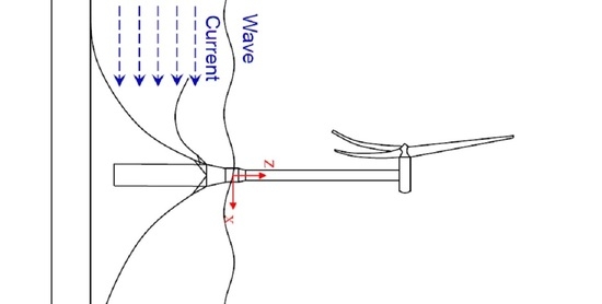
A regular wave test for the 6MW spar-type FOWT was performed in the State Key Laboratory of Ocean Engineering (SKLOE) at Shanghai Jiao Tong University. The wave tank is of length 50 m and width 4 m, respectively. In addition, a 1: 65.3 scale model of the 6 MW spar-type FOWT was built and tested without considering current or forward speed effects. The general layout for the experiment set up is shown in Figure 12. The wave parameters at full scale and model scale are presented in Table 3.
5.3. Validation against Model Test in a Regular Wave
Numerical analysis has been carried out up to the 2nd order using the same spar geometry, loading condition, and the wave conditions described previously in Section 5.1 and Section 5.2. The numerical results will be compared with that of the model test in Yao et al. [48]. The hydrodynamic mesh model of the full-scale 6 MW spar-type FOWT generated from GMSH [49] is shown in Figure 13. A free-surface mesh with a radius of 1200 m is used, where a damping zone starting from 400 meters is applied to absorb the diffracted and radiated waves. It means that we are using a ring-type damping zone layer with a width of 800 m, which has been shown to be sufficient to absorb most of the energy of the outgoing scatter waves. There are 21 patches along the vertical direction of the body surface. In addition, 32 and 41 patches are used along the circumferential and radial directions respectively to assure enough resolution for both free surface and body surface. In addition, finer meshes are adopted near the waterline both on the free surface and body surface. Furthermore, at least 30 patches along the radial direction per wave length in the near field are modeled. To this end, the final mesh model contains 1932 cubic patches and 9703 nodes.
For simplicity in numerical modeling while keeping the spar-type FOWT in an acceptable position, the catenary mooring line theory described in Section 3.2 is applied. Therefore, mooring dynamics are not modeled, whose effects will be investigated in future studies. When it is relevant, drag loads based on Morison’s equation and relative velocities are also included as part of the hydrodynamic loads. See the description in Section 3.3.
In order to examine the importance of the mooring and drag loads, three cases summarized in Table 4 will be studied. The first case does not apply any mooring or viscous drag loads. A long ramp period has been used to gradually start the simulation, in order to minimize the horizontal drifting of the FOWT. The second case includes a catenary mooring model, but without any viscous drag loads. In the third case, catenary mooring and viscous drag loads (on the spar-type FOWT but not the mooring lines) are both included. The quadratic terms in Equations (27) and (28) have been included in the calculation of hydrodynamic responses of the FOWT.
The surge, heave, and pitch motion results are presented in Figure 14. The figures on the left are the 1st-order or total results in comparison with experimental measurements. The corresponding 2nd-order components of the numerical results are presented in the figures in the right column. In the figures, the results for the three cases are denoted by ‘Method 1’, ‘Method 2’, and ‘Method 3’, respectively. To make better comparisons, we have shifted the linear numerical results for Method 2 and Method 3 by a phase angle of relative to that of Method 1. For the same reason, the 2nd-order results have also been shifted by for those two cases.
As seen from Figure 14, results for Method 2 and Method 3 show very little differences, indicating that the viscous drag loads are less important. However, one should note that the viscous drag may be important for the accurate approximation of the hydrodynamic response of the FOWTs if much larger waves are considered.
It can also be seen from the heave motion in Figure 14 that the calculations by these three methods all agree well with the experiment results. Some non-negligible influences of the mooring system for surge motion are seen. In fact, when no mooring restoring is included, our numerical results agree fairly well with the experimental results, while the results with mooring unexpectedly deviate more from the experiment. The numerical results by the time-domain coupled simulation tool FAST presented in [48] also showed the same tendency. It was mentioned by Yao et al. [48] that the cable bundle that powered the turbine in the experiment may have had non-negligible effects. Furthermore, the amplitude of the 2nd-order sum-frequency responses seem to be small compared to the corresponding linear components.
In Figure 15, the linear Response Amplitude Operators (RAOs) for waves from shorter to longer waves lengths are presented. They are obtained as the 1st harmonics from the time series. For Method 3, the drag loads have been calculated by assuming a wave steepness . In general, the viscous drag loads have very little influence for the considered FOWTs and wave conditions. For long waves, the mooring system is seen to have some non-negligible effect on surge motions.
The non-dimensional mean-drift force are compared in Figure 16, where results for Method 2 and Method 3 with and are included. The 3rd-order terms in Equations (27) and (28) are included in the calculation of the mean-drift forces. Since the mean-drift force is normalized by , the non-dimensional total mean-drift forces are dependent on . For small wave steepness , the results are very close to that of Method 2 (no viscous drag at all), while clear increases of mean-drift force are seen for due to the viscous-drag contribution.
5.4. Current Effect
Based on the understanding from the three models in Section 5.3, we will use Method 2 to carry out further numerical analyses to investigate the current effect on the 6 MW spar-type FOWT foundation. The same mesh model and numerical method (see Section 3.3) are employed for the present study. Uniform current with is considered, where m is the radius of the circular water-plane. It corresponds to current speed of m/s, which is not considered as excessively large on typical offshore sites. Here, as a definition, a positive number means that the current is in the opposite direction as the wave propagation direction. A non-uniform current cannot be modeled in the present potential-flow model, as a circulation must have been created due to a non-uniform current, leading to a rotational flow. In fact, ocean currents are ubiquitous in real sea and usually generated by winds, tides, or thermal gradients.
The solutions of 1st-order motions and horizontal mean-drift force of the spar platform in the time domain can be transformed into RAOs and quadratic transform functions (QTFs) in the frequency domain, respectively. The motion RAOs and the inline mean-drift force QTF are presented in Figure 17 and Figure 18, respectively.
The RAOs shown in Figure 17 demonstrate the decrease of motions in surge, heave, and pitch modes with the increase of for the spar platform for cases with zero forward speed or under current speeds. An increase of the response was captured in long waves for the three motion modes when the current speed is in the opposite direction of the wave propagation, i.e., . In this case, the encounter frequency is smaller than the wave frequency, and thus are closer to the resonant frequencies. According to the experimental results in Yao et al. [48], the surge, heave and pitch natural periods of the considered spar-type FOWT are s, s and s, respectively.
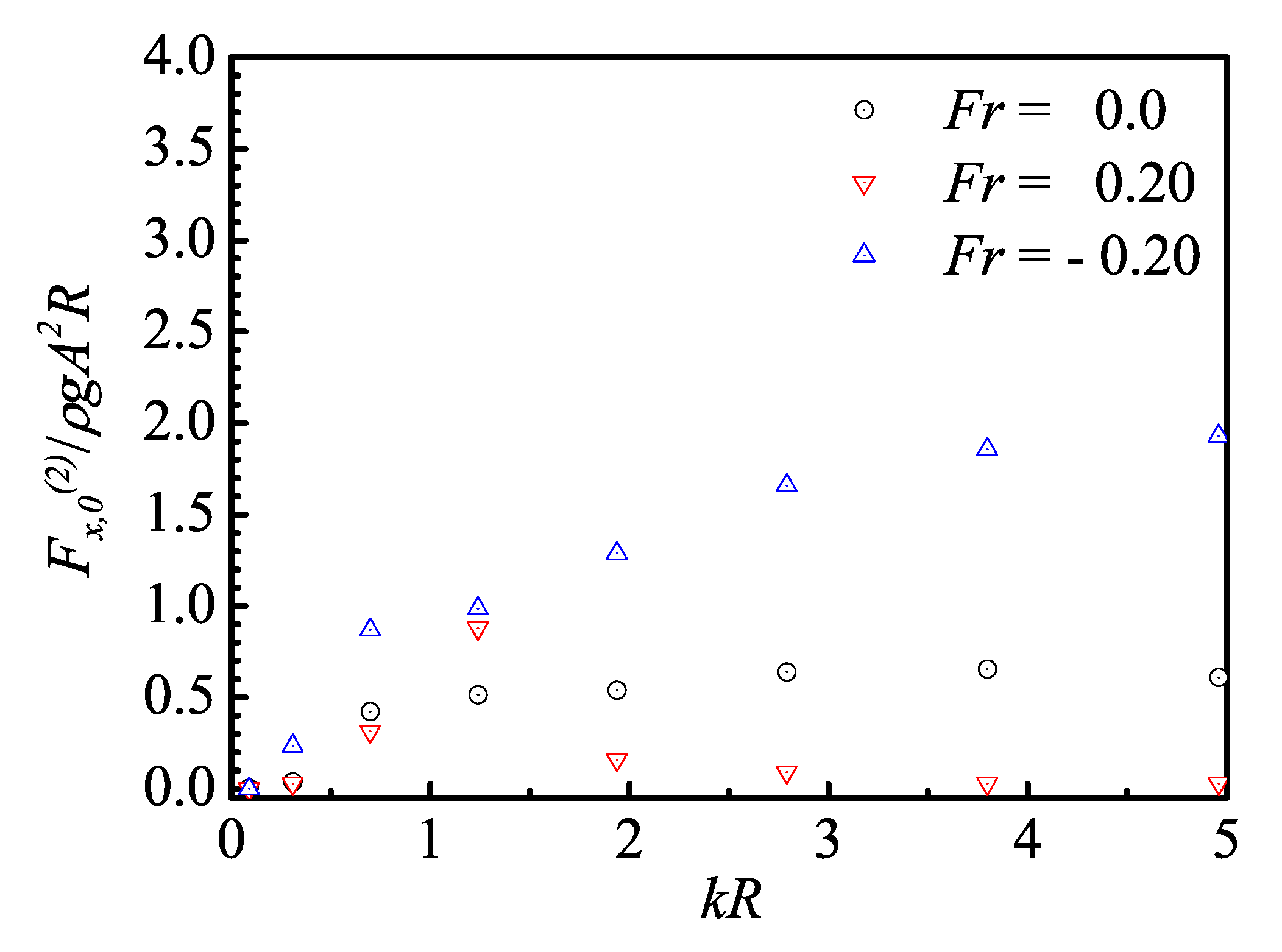
The inline horizontal mean-drift forces of the 6MW spar-type FOWT are presented in Figure 18. In general, the inline mean-drift force is larger when the wave propagates in the same direction as the current. The current effect is in general significant. Since the mean-drift force is a special case of the difference-frequency force, the results indicate that it may be important to include the current effects in the evaluation of the slowly-varying wave loads and the slow-drift motions.
6. Conclusions and Future Work
A complete 2nd-order wave–current–structure interaction model has been presented. The numerical model is firstly verified against reference cases with benchmark results available in the literature. Then, the model is applied to study the hydrodynamic characteristics of a 6 WM spar-type FOWT. The wind loads are not included in the present stage. Quasi-static mooring loads are modeled via the catenary line theory, and drag loads are empirically accounted for by the Morison’s equation. For the considered 6 MW spar-type FOWT, the model is validated against model tests under a regular wave excitation with a wave period of 15 s and wave height of 10 m. The complete 2nd-order problems were solved and satisfactory agreement has been achieved between numerical results and experiments. The 2nd-order sum-frequency effects were found to be inconsequential for the FOWT motion responses under the considered wave conditions, and the viscous-drag loads as well. However, the 3rd order viscous drag clearly increases the mean-drift forces with an increasing wave steepness. Furthermore, the hydrodynamics responses of this FOWT in the presence of either a small positive or a reverse uniform current are numerically investigated. The influence of the current on 1st-order RAOs is mainly embodied at low frequencies, whereas the mean-drift forces are strongly affected by the magnitude and direction of the uniform current.
In future studies, a more accurate mooring dynamics model will be adopted to replace the catenary line model. The present complete 2nd-order time-domain model will also be extended to simulate the dynamic responses of the FOWTs in irregular waves. The wind loads should also be included in order to render the numerical simulations more realistic.
Author Contributions
Conceptualization, Y.S.; methodology, Y.S. and Z.Z.; software, Y.S., Z.Z., and J.C. validation, Y.S. and Z.Z.; formal analysis, H.L. and Y.Z.; investigation, Y.S., Z.Z., and Y.Z.; writing-original draft preparation, Z.Z.; writing-review and editing, Y.S., H.L., and J.C.; supervision, Y.S. and J.C.; project administration, J.C. All authors have approved the contents of the submitted manuscript.
Funding
J.C. acknowledges the financial support from the National Science Foundation of China (Grant No. 51709064).
Conflicts of Interest
The authors declare no conflict of interests.
Appendix A
The hydrodynamic forces and moments acting on the body surface at specific-order can be approximated based on the method of direct pressure integration:
where and , are the forces and moments of k-th order by applying Taylor expansion method. is the position vector of a point on the body surface. with is the free-surface elevation at the specific order. denotes the still waterline and the integral on the still waterline is due to the small variation of the instantaneous body surface and mean body surface induced by the body motions and free-surface elevation. is the normal vector of a point on the body surface and is given as . are the normal vectors due to coordinate transformation and are in magnitude of and , respectively.
Appendix B
Applying the standard implicit Euler method, one can discretize Equation (36) as
where the advection term is discretized using the solution at the current time step, i.e., . N is the total number of grid points. is the operator for the spatial differentiation , based on standard finite difference schemes or any other velocity reconstruction methods using stencil points around the grid points of interest. is dependent on the size of meshes, thus we introduce a characteristic mesh size and rewrite Equation (A7) as
where
and
Here, r is propositional to the number. The scaled operator has less dependence on grid size than the un-scaled operator .
After considering proper boundary conditions at two ends of the domain, we can formally set up a matrix equation for the solution at -th time step
Here, is identity matrix. is a sparse matrix whose bandwidth is equal to the size of local stencil points. The standard way of solving Equation (A11) is to solve the sparse-matrix equation iteratively, which may be computationally costly as the matrix on the left-hand side is not diagonal-dominant. Considering r as a small parameter, e.g., , we can approximate the inverse of by series expansion in r
Here, the matrix with are independent on r. To determine , we take the product of and :
Requiring each term in Equation (A14) to vanish leads to a simple solution for . Therefore, an explicit approximation for can be obtained as
where we have truncated the infinite series summation to terms. To this end, we can approximate the implicit Euler scheme as
which is an explicit scheme and conditionally stable as it is shown in Shao [38] in the stability analysis.
A similar procedure can be followed to approximate other implicit schemes. The results for the 2nd-order Crank–Nicolson scheme is shown in Equation (37), which is used throughout this study.
References
- Fulton, G.; Malcolm, D.; Moroz, E. Design of a semi-submersible platform for a 5MW wind turbine. In Proceedings of the 44th AIAA Aerospace Sciences Meeting and Exhibit, Reno, NV, USA, 9–12 January 2006; p. 997. [Google Scholar]
- Butterfield, S.; Musial, W.; Jonkman, J.; Sclavounos, P. Engineering Challenges for Floating Offshore Wind Turbines; Technical Report; National Renewable Energy Lab. (NREL): Golden, CO, USA, 2007.
- Robertson, A.N.; Jonkman, J.M.; Goupee, A.J.; Coulling, A.J.; Prowell, I.; Browning, J.; Masciola, M.D.; Molta, P. Summary of conclusions and recommendations drawn from the DeepCwind scaled floating offshore wind system test campaign. Int. Conf. Offshore Mech. Arct. Eng. Am. Soc. Mech. Eng. 2013, 55423, V008T09A053. [Google Scholar]
- Coulling, A.J.; Goupee, A.J.; Robertson, A.N.; Jonkman, J.M.; Dagher, H.J. Validation of a FAST semi-submersible floating wind turbine numerical model with DeepCwind test data. J. Renew. Sustain. Energy 2013, 5, 023116. [Google Scholar] [CrossRef]
- Browning, J.; Jonkman, J.; Robertson, A.; Goupee, A. Calibration and validation of a spar-type floating offshore wind turbine model using the FAST dynamic simulation tool. In Journal of Physics: Conference Series; IOP Publishing: Bristol, UK, 2014; Volume 555, p. 012015. [Google Scholar]
- Driscoll, F.; Jonkman, J.; Robertson, A.; Sirnivas, S.; Skaare, B.; Nielsen, F.G. Validation of a FAST model of the statoil-hywind demo floating wind turbine. Energy Procedia 2016, 94, 3–19. [Google Scholar] [CrossRef] [Green Version]
- Utsonomiya, T.; Sato, T.; Matsukuma, H.; Yago, K. Experimental validation for motion of a spar- type floating offshorewind turbine using 1/22.5 scale model. In International Conference on Ocean, Offshore and Arctic Engineering (OMAE2020) International Conference on Ocean, Offshore and Arctic Engineering; American Society of Mechanical Engineers: New York, NY, USA, 2009. [Google Scholar]
- Robertson, A.; Jonkman, J.; Masciola, M.; Song, H.; Goupee, A.; Coulling, A.; Luan, C. Definition of the Semisubmersible Floating System for Phase II of OC4; Technical Report; National Renewable Energy Lab. (NREL): Golden, CO, USA, 2014.
- Benitz, M.A.; Schmidt, D.P.; Lackner, M.A.; Stewart, G.M.; Jonkman, J.; Robertson, A. Validation of hydrodynamic load models using CFD for the OC4-DeepCwind semisubmersible. In International Conference on Offshore Mechanics and Arctic Engineering; American Society of Mechanical Engineers: New York, NY, USA, 2015; Volume 56574, p. V009T09A037. [Google Scholar]
- Robertson, A.N.; Jonkman, J.M. Loads analysis of several offshore floating wind turbine concepts. In Proceedings of the Twenty-First, International Offshore and Polar Engineering Conference, Maui, HI, USA, 19–24 June 2011. [Google Scholar]
- Goupee, A.J.; Koo, B.; Lambrakos, K.; Kimball, R. Model tests for three floating wind turbine concepts. In Proceedings of the Offshore Technology Conference, Houston, TX, USA, 30 April–3 May 2012. [Google Scholar]
- Jonkman, J. Definition of the Floating System for Phase IV of OC3; Technical Report; National Renewable Energy Lab. (NREL): Golden, CO, USA, 2010.
- Tomasicchio, G.R.; Armenio, E.; D’Alessandro, F.; Fonseca, N.; Mavrakos, S.A.; Penchev, V.; Jensen, P. Design of a 3D physical and numerical experiment on floating off-shore wind turbines. Coast. Eng. Proc. 2012, 1, 67. [Google Scholar] [CrossRef]
- Tomasicchio, G.R.; D’Alessandro, F.; Avossa, A.M.; Riefolo, L.; Musci, E.; Ricciardelli, F.; Vicinanza, D. Experimental modelling of the dynamic behaviour of a spar buoy wind turbine. Renew. Energy 2018, 127, 412–432. [Google Scholar] [CrossRef]
- Shin, H. Model test of the OC3-Hywind floating offshore wind turbine. In Proceedings of the Twenty-first International Offshore and Polar Engineering Conference, Maui, HI, USA, 19–24 June 2011. [Google Scholar]
- Ogilvie, T.F. Second-order hydrodynamic effects on ocean platforms. In Proceedings of the International Workshop on Ship and Platform Motions, Berkeley, CA, USA, 26–28 October 1983; pp. 205–265. [Google Scholar]
- Newman, J. The second-order wave force on a vertical cylinder. J. Fluid Mech. 1996, 320, 417–443. [Google Scholar] [CrossRef]
- Roald, L.; Jonkman, J.; Robertson, A.; Chokani, N. The effect of second-order hydrodynamics on floating offshore wind turbines. Energy Procedia 2013, 35, 253–264. [Google Scholar] [CrossRef] [Green Version]
- Meng, L.; He, Y.; Zhou, T.; Zhao, Y.; Liu, Y. Research on Dynamic Response Characteristics of 6MW Spar-Type Floating Offshore Wind Turbine. J. Shanghai Jiaotong Univ. (Sci.) 2018, 23, 505–514. [Google Scholar] [CrossRef]
- Coulling, A.J.; Goupee, A.J.; Robertson, A.N.; Jonkman, J.M. Importance of second-order difference-frequency wave-diffraction forces in the validation of a fast semi-submersible floating wind turbine model. In International Conference on Offshore Mechanics and Arctic Engineering; American Society of Mechanical Engineers: New York, NY, USA, 2013; Volume 55423, p. V008T09A019. [Google Scholar]
- Gueydon, S.; Duarte, T.; Jonkman, J. Comparison of second-order loads on a semisubmersible floating wind turbine. In International Conference on Offshore Mechanics and Arctic Engineering; American Society of Mechanical Engineers: New York, NY, USA, 2014; Volume 45530, p. V09AT09A024. [Google Scholar]
- Zhang, L.; Shi, W.; Karimirad, M.; Michailides, C.; Jiang, Z. Second-order hydrodynamic effects on the response of three semisubmersible floating offshore wind turbines. Ocean Eng. 2020, 207, 107371. [Google Scholar] [CrossRef]
- Bae, Y.; Kim, M. Rotor-floater-tether coupled dynamics including second-order sum–frequency wave loads for a mono-column-TLP-type FOWT (floating offshore wind turbine). Ocean Eng. 2013, 61, 109–122. [Google Scholar] [CrossRef]
- Gueydon, S.; Jonkman, J. Update on the Comparison of Second-Order Loads on a Tension Leg Platform for Wind Turbines; Technical Report; National Renewable Energy Lab. (NREL): Golden, CO, USA, 2016.
- Li, Y.; Tang, Y.; Zhu, Q.; Qu, X.; Wang, B.; Zhang, R. Effects of second-order wave forces and aerodynamic forces on dynamic responses of a TLP-type floating offshore wind turbine considering the set-down motion. J. Renew. Sustain. Energy 2017, 9, 063302. [Google Scholar] [CrossRef]
- Jonkman, J.M. Dynamics Modeling and Loads Analysis of an Offshore Floating Wind Turbine; Technical Report; National Renewable Energy Lab. (NREL): Golden, CO, USA, 2007.
- Bayati, I.; Jonkman, J.; Robertson, A.; Platt, A. The effects of second-order hydrodynamics on a semisubmersible floating offshore wind turbine. In Journal of Physics: Conference Series; IOP Publishing: Bristol, UK, 2014; Volume 524, pp. 1–10. [Google Scholar]
- Wolfram, J. On alternative approaches to linearization and Morison’s equation for wave forces. Proc. R. Soc. Lond. A 1999, 157, 2957–2974. [Google Scholar] [CrossRef]
- Shao, Y.; You, J.; Glomnes, E.B. Stochastic linearization and its application in motion analysis of cylindrical floating structure with bilge boxes. In Proceedings of the 35th International Conference on Ocean, Offshore and Arctic Engineering, Busan, Korea, 19–24 June 2016. [Google Scholar]
- Lin, Y.; El Chahal, G.; Shao, Y. Caisson Breakwater for LNG & Bulk Terminals: A Study on Limiting Wave Conditions for Caisson Installation. In Proceedings of the 39th International Conference on Ocean, Offshore and Arctic Engineering (OMAE2020), Fort Lauderdale, FL, USA, 28 June–3 July 2020. [Google Scholar]
- Shao, Y.; Faltinsen, O.M. Use of body-fixed coordinate system in analysis of weakly nonlinear wave–body problems. Appl. Ocean Res. 2010, 32, 20–33. [Google Scholar] [CrossRef]
- Bai, W.; Teng, B. Simulation of second-order wave interaction with fixed and floating structures in time domain. Ocean Eng. 2013, 74, 168–177. [Google Scholar] [CrossRef]
- Duan, W.; Chen, J.; Zhao, B. Second-order Taylor expansion boundary element method for the second-order wave radiation problem. Appl. Ocean Res. 2015, 52, 12–26. [Google Scholar] [CrossRef]
- Shao, Y.; Faltinsen, O. Numerical Study on the Second-Order Radiation/Diffraction of Floating Bodies with/without Forward Speed. In Proceedings of the 25th International Workshop on Water Waves and Floating Bodies (IWWWFB 2010), Harbin, China, 9–12 May 2010. [Google Scholar]
- Shao, Y.L.; Faltinsen, O.M. Second-order diffraction and radiation of a floating body with small forward speed. J. Offshore Mech. Arct. Eng. 2013, 135, 011301. [Google Scholar] [CrossRef]
- Shao, Y.; Faltinsen, O.M. A numerical study of the second-order wave excitation of ship springing by a higher-order boundary element method. Int. J. Nav. Archit. Ocean Eng. 2014, 4, 1000–1013. [Google Scholar] [CrossRef] [Green Version]
- Teng, B.; Jin, R.; Cong, L. A twice expansion analysis method in the time-domain for wave action on a floater translating with a large amplitude. Ocean Eng. 2016, 118, 138–151. [Google Scholar] [CrossRef]
- Shao, Y. On a new explicit time-integration method for advection equation and its application in hydrodynamics. In Proceedings of the 35th International Workshop on Water Waves and Floating Bodies (IWWWFB 2020), Seoul, Korea, 24–28 August 2020. [Google Scholar]
- Faltinsen, O.M.; Timokha, A.N. Sloshing; Cambridge University Press: Cambridge, UK, 2009; Volume 577. [Google Scholar]
- Shao, Y. Numerical Potential-Flow Studies on Weakly-Nonlinear Wave-Body Interactions with/without Small Forward Speeds. Ph.D. Thesis, Norwegian University of Science and Technology, Trondheim, Norway, 2010. [Google Scholar]
- Feng, A.; Kang, H.S.; Zhao, B.; Jiang, Z. Two-Dimensional Numerical Modelling of a Moored Floating Body under Sloping Seabed Conditions. J. Mar. Sci. Eng. 2020, 8, 389. [Google Scholar] [CrossRef]
- Faltinsen, O.M. Sea Loads on Ships and Offshore Structures; Cambridge University Press: Cambridge, UK, 1990. [Google Scholar]
- Kring, D. Time Domain Ship Motions by a Three-Dimensional Rankine Panel Method. Ph.D. Thesis, Massachusetts Institute of Technology, Cambridge, MA, USA, 1994. [Google Scholar]
- Savitzky, A.; Golay, M.J.E. Smoothing and differentiation of data by simplified least squares procedures. Anal. Chem. 1964, 36, 1627–1639. [Google Scholar] [CrossRef]
- Newman, J.N. Transient axisymmetric motion of a floating cylinder. J. Fluid Mech. 1985, 157, 17–33. [Google Scholar] [CrossRef]
- Drake, K.R. An analytical approximation for the horizontal drift force acting on a deep draught spar in regular waves. Ocean Eng. 2011, 38, 810–814. [Google Scholar] [CrossRef]
- Malenica, S.; Clark, P.J.; Molin, B. Wave and current forces on a vertical cylinder free to surge and sway. Appl. Ocean Res. 1995, 17, 79–90. [Google Scholar] [CrossRef]
- Yao, T.C.; Zhao, Y.S.; He, Y.P.; Shao, Y.L.; Han, Z.L.; Duan, L. CFD-based Analysis of a 6MW Spar-type Floating Wind Turbine with Focus on Nonlinear Wave Loads. In Proceedings of the 30th International Ocean and Polar Engineering Conference, Shanghai, China, 11–16 October 2020. [Google Scholar]
- Geuzaine, C.; Remacle, J.-F. R. Gmsh: A 3D finite element mesh generator with built-in pre-and post-processing facilities. Int. J. Numer. Methods Eng. 2009, 79, 1309–1331. [Google Scholar] [CrossRef]
Figure 1.
Definition of three coordinate systems: , and .
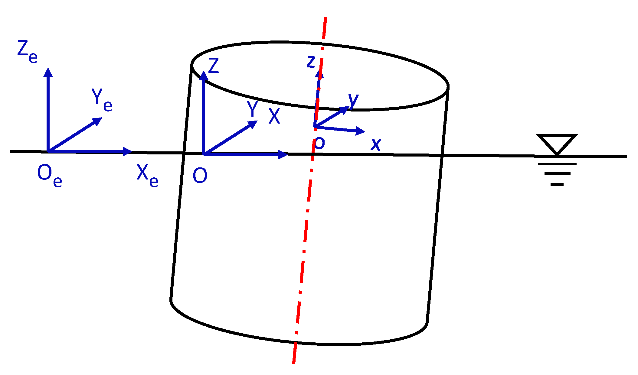
Figure 2.
Definition of the free-surface elevations observed in OXYZ and oxyz systems.

Figure 3.
Representation of 12-node cubic patch in physical plane and parametric plane.
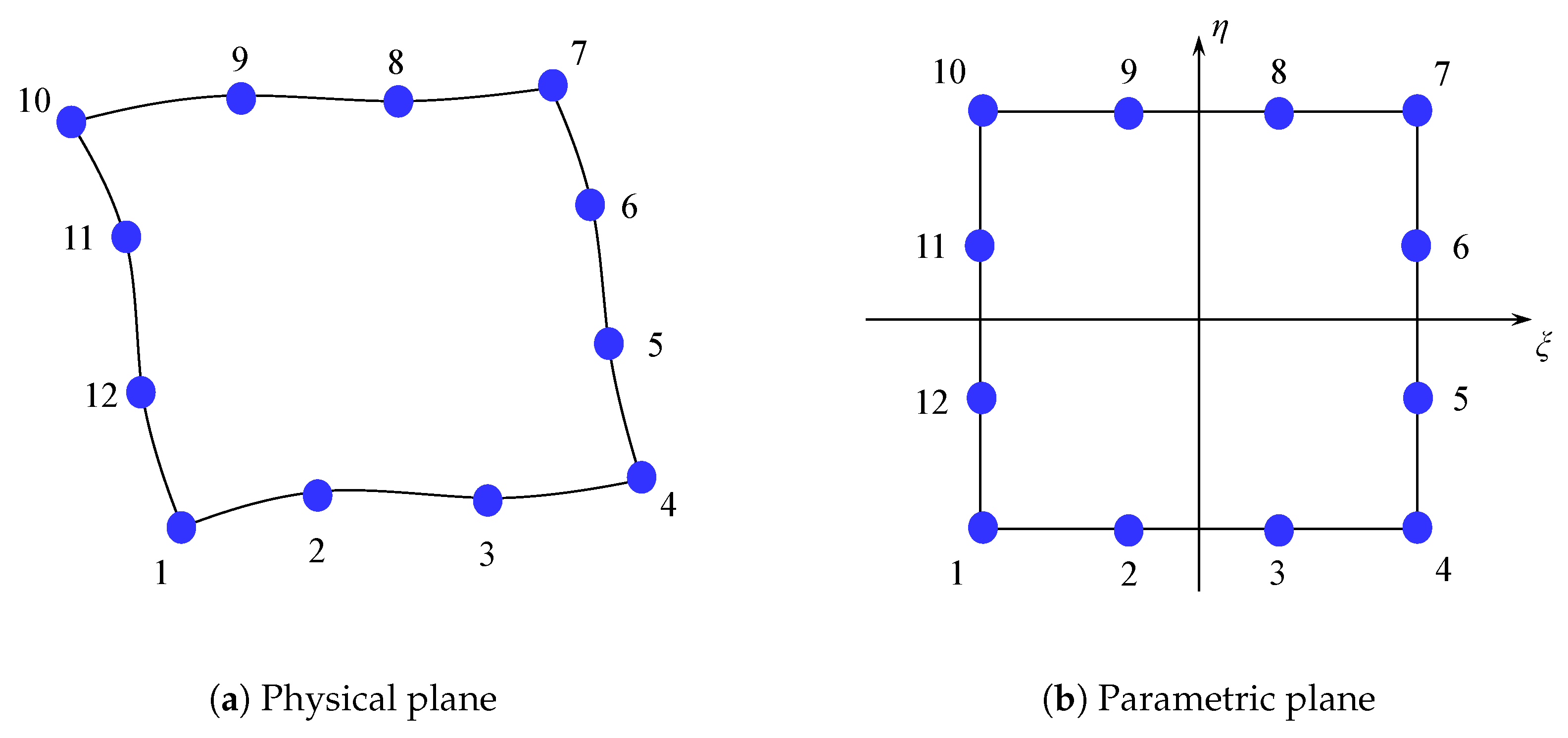
Figure 4.
Sketch of catenary mooring line model in the 2D plane.
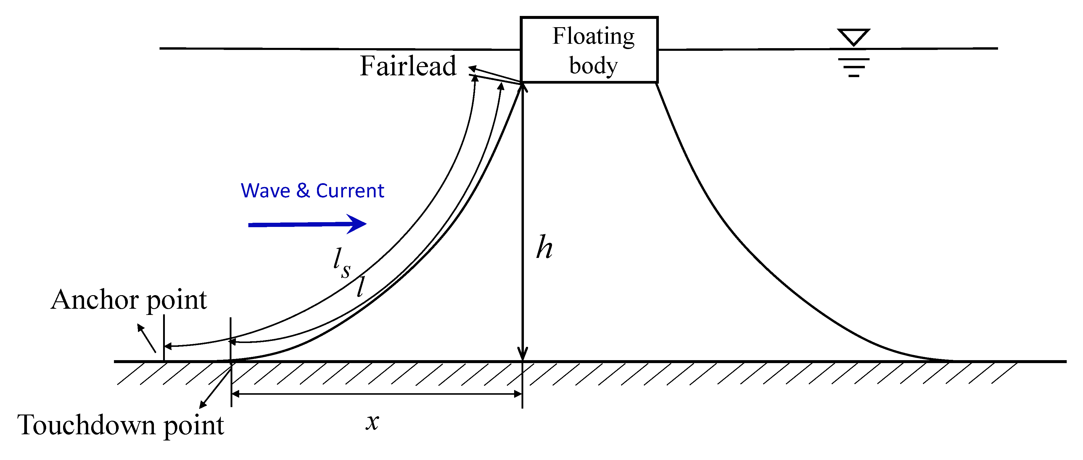
Figure 5.
Time history of vertical displacement of a freely floating truncated vertical cylinder specifying initial motion.
Figure 5.
Time history of vertical displacement of a freely floating truncated vertical cylinder specifying initial motion.
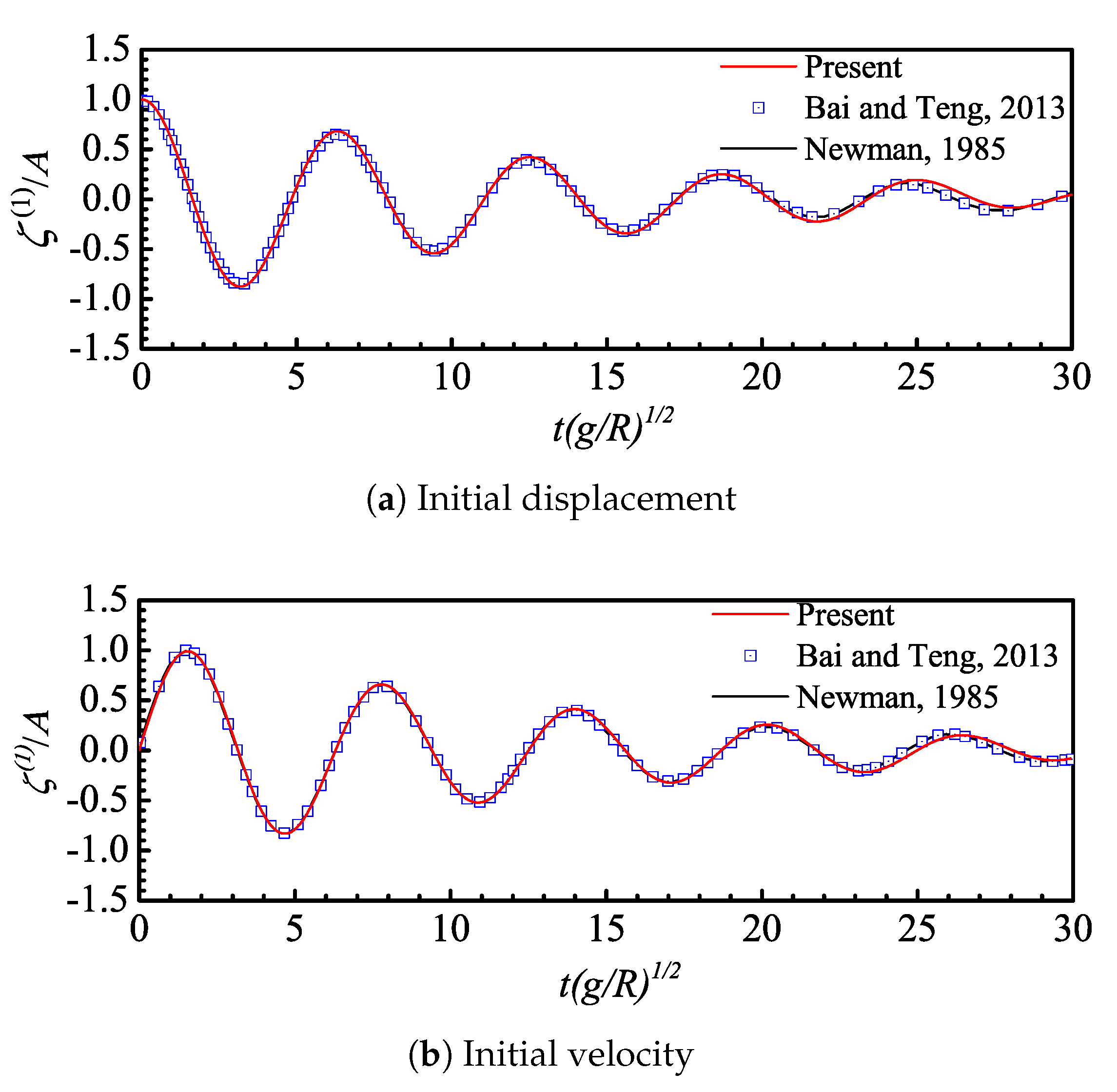
Figure 6.
Time history of hydrodynamic force on a freely floating truncated vertical cylinder specifying initial motion.
Figure 6.
Time history of hydrodynamic force on a freely floating truncated vertical cylinder specifying initial motion.
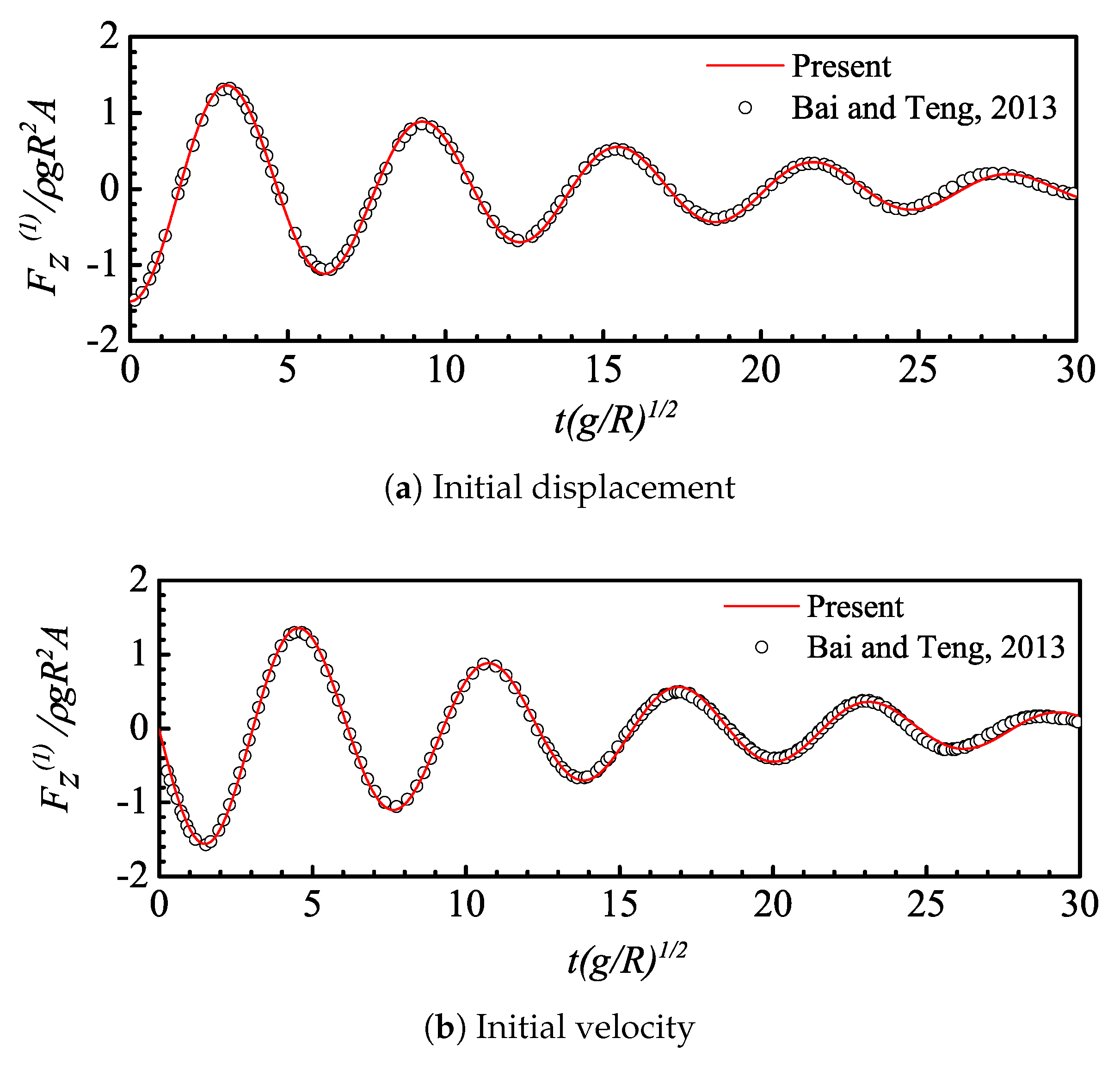
Figure 7.
Lateral displacement of spar at still waterline and the base: upper line and symbols for still waterline; lower line and symbols for the base.
Figure 7.
Lateral displacement of spar at still waterline and the base: upper line and symbols for still waterline; lower line and symbols for the base.
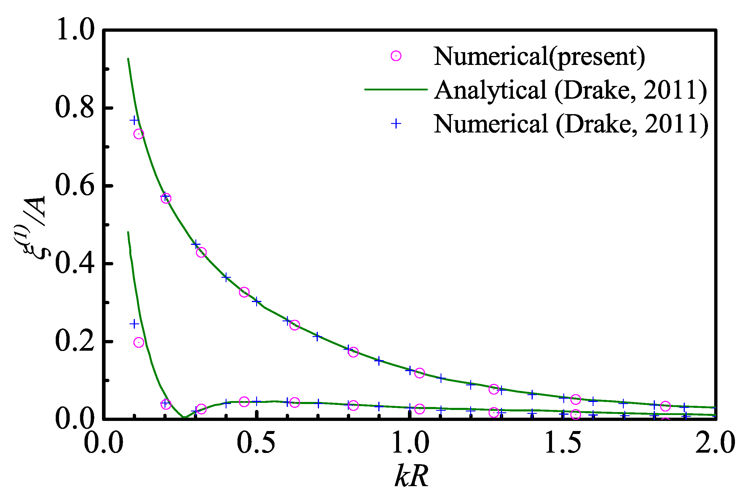
Figure 8.
Horizontal wave-drift forces acting on the cylinder.

Figure 9.
The 1st-order surge motion amplitude of the vertical cylinder at a forward speed.

Figure 10.
Spar platform of the 6MW spar-type FOWT.
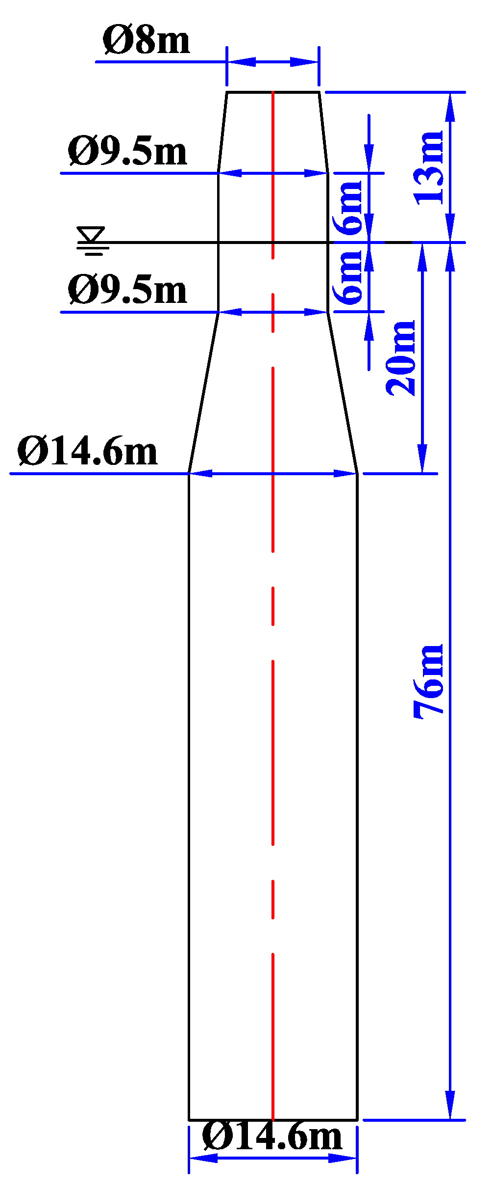
Figure 11.
Sketch of catenary mooring system of the 6 MW spar-type FOWT.
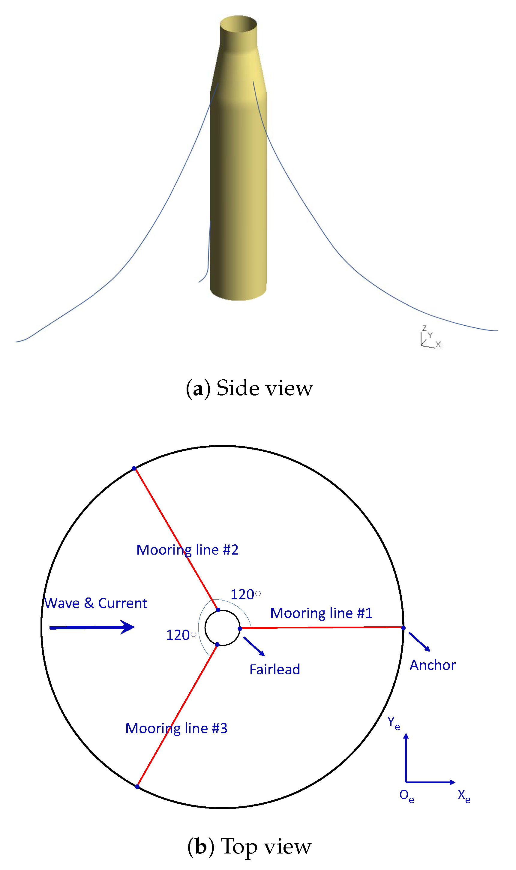
Figure 12.
General layout for the experiment test.
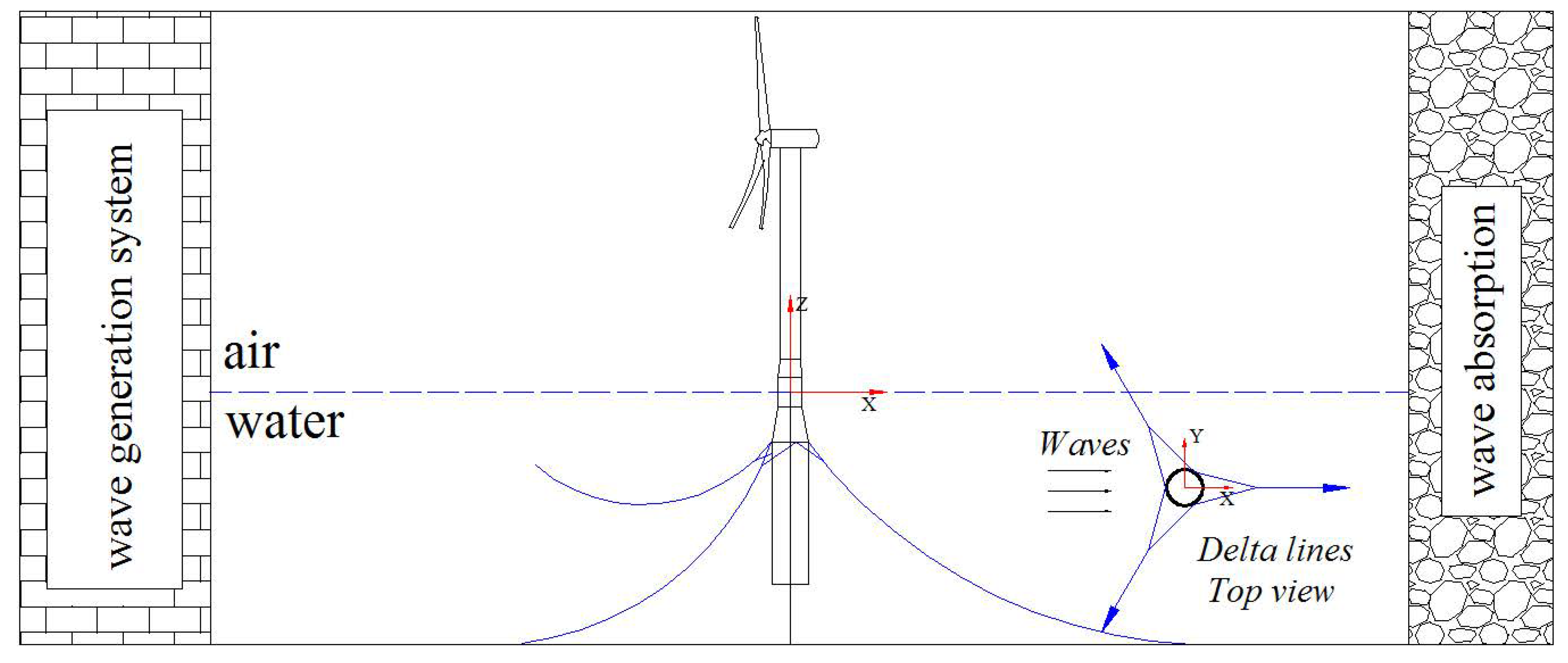
Figure 13.
Example of mesh models on the free surface and the substructure of the 6 MW spar-type FOWT.
Figure 13.
Example of mesh models on the free surface and the substructure of the 6 MW spar-type FOWT.

Figure 14.
The 1st- and 2nd-order time series of the responses of the 6MW spar-type FOWT. The (left) column exhibits the comparison between the present results and experiments from [48]. Here, legends of figures only represent different methods. In addition, the solid lines () are drawn for 1st-order results while the dotted lines () are for results with the 2nd-order components included. The (right) column only displays the 2nd-order results determined by different methods.
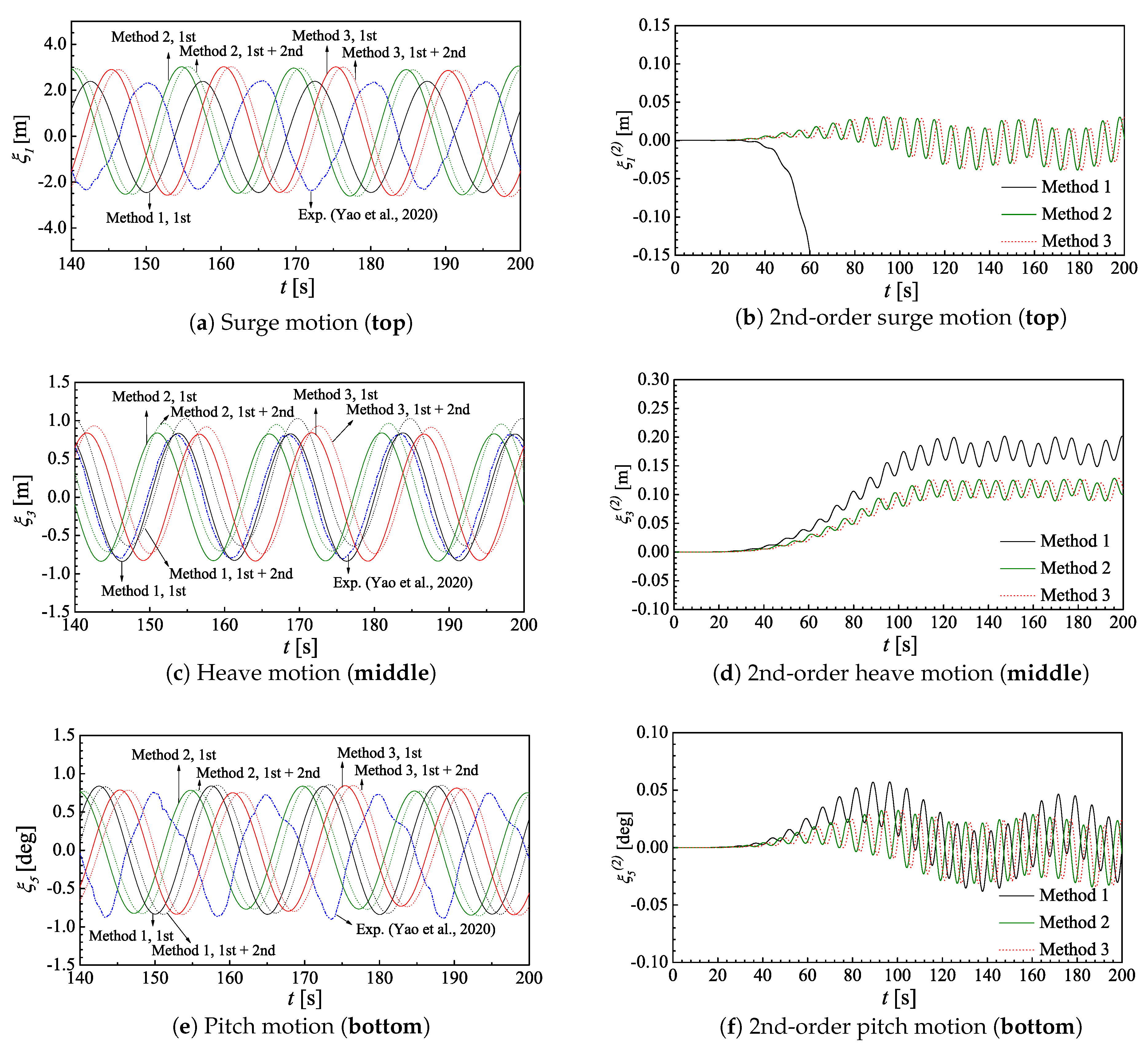
Figure 15.
The 1st-order surge, heave and pitch motion RAOs of the 6MW spar-type FOWT by different methods.
Figure 15.
The 1st-order surge, heave and pitch motion RAOs of the 6MW spar-type FOWT by different methods.
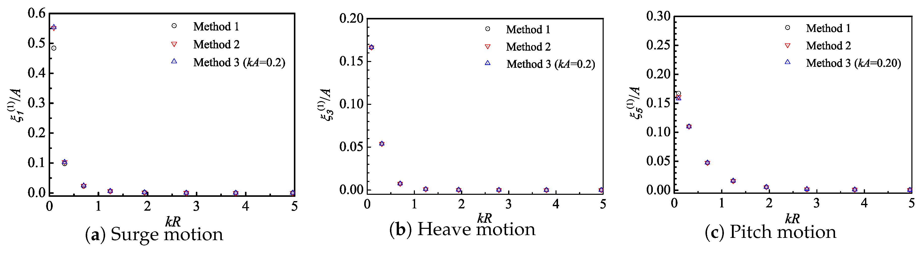
Figure 16.
Horizontal mean-drift force of the 6MW spar-type FOWT.
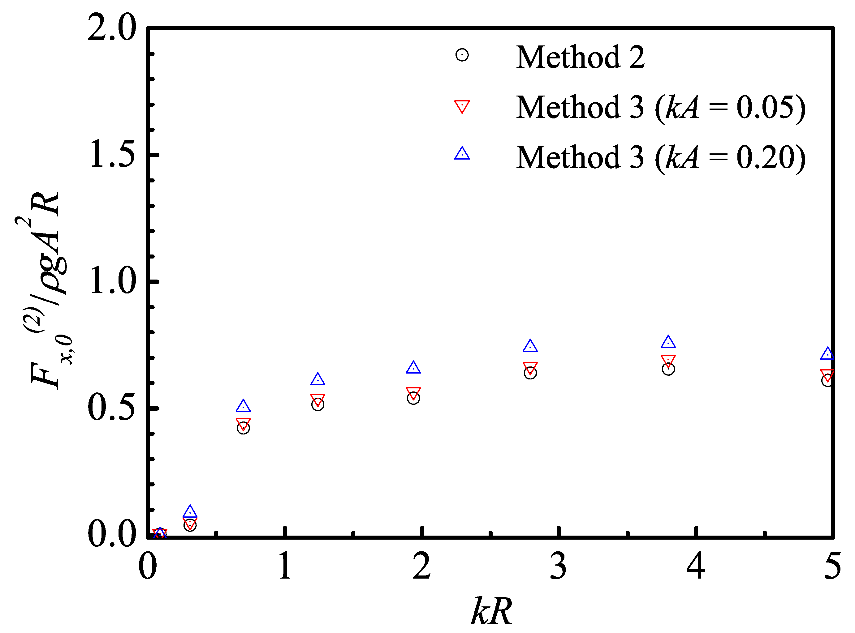
Figure 17.
The 1st-order motion RAOs of the 6MW spar-type FOWT at different Froude numbers. Note that the problem of a body undergoing a positive forward speed in waves is equivalent to the problem of a body in waves and negative current by neglecting the interaction between the wave and current.
Figure 17.
The 1st-order motion RAOs of the 6MW spar-type FOWT at different Froude numbers. Note that the problem of a body undergoing a positive forward speed in waves is equivalent to the problem of a body in waves and negative current by neglecting the interaction between the wave and current.
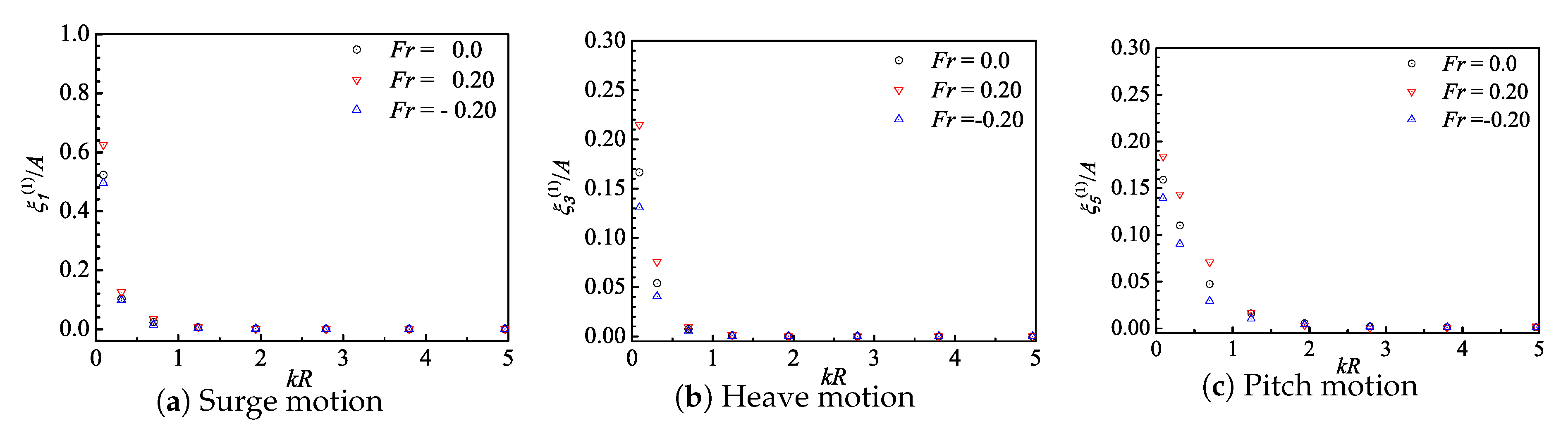
Figure 18.
Horizontal mean-drift force of the 6MW spar-type FOWT for , and .

Table 1.
Main parameters of the spar platform of a 6MW spar-type FOWT in full scale.
| Water depth [m] | 100 |
| Draft [m] | 76 |
| Mass [t] | 11,137 |
| Displacement [m3] | 11,420 |
| Center of gravity [m] | −49 |
| Moment of inertia(roll, pitch) [kg m2] | 4.20 × |
Table 2.
Main properties of the mooring lines.
| Number of mooring lines | 3 |
| Angle between mooring lines [deg] | 120 |
| Unstretched mooring line length [m] | 400 |
| Radius of fairleads to centerline [m] | 8 |
| Radius of anchors to centerline [m] | 393.5 |
| Depth of fairleads [m] | 21 |
| Depth of anchors [m] | 100 |
| Extensional stiffness(EA) [N/m] | 8.0 × |
| Mass per unit length [kg m−1] | 370 |
Table 3.
Regular wave parameters for model-scale and full-scale models.
| Water Depth [m] | Wave Height [m] | Wave Period [s] | Wave Length [m] | |
|---|---|---|---|---|
| Full scale | 100 | 10 | 15 | 338 |
| Model scale (1:65.3) | 1.53 | 0.153 | 1.856 | 5.171 |
Table 4.
Load cases and setup.
| Cases | Case Setup |
|---|---|
| Method 1 | Ramp periods = 8T |
| Method 2 | Catenary mooring |
| Method 3 | Catenary mooring + Viscous drag |
Publisher’s Note: MDPI stays neutral with regard to jurisdictional claims in published maps and institutional affiliations. |
© 2020 by the authors. Licensee MDPI, Basel, Switzerland. This article is an open access article distributed under the terms and conditions of the Creative Commons Attribution (CC BY) license (http://creativecommons.org/licenses/by/4.0/).
Share and Cite
MDPI and ACS Style
Zheng, Z.; Chen, J.; Liang, H.; Zhao, Y.; Shao, Y. Hydrodynamic Responses of a 6 MW Spar-Type Floating Offshore Wind Turbine in Regular Waves and Uniform Current. Fluids 2020, 5, 187. https://doi.org/10.3390/fluids5040187
AMA Style
Zheng Z, Chen J, Liang H, Zhao Y, Shao Y. Hydrodynamic Responses of a 6 MW Spar-Type Floating Offshore Wind Turbine in Regular Waves and Uniform Current. Fluids. 2020; 5(4):187. https://doi.org/10.3390/fluids5040187
Chicago/Turabian StyleZheng, Zhiping, Jikang Chen, Hui Liang, Yongsheng Zhao, and Yanlin Shao. 2020. "Hydrodynamic Responses of a 6 MW Spar-Type Floating Offshore Wind Turbine in Regular Waves and Uniform Current" Fluids 5, no. 4: 187. https://doi.org/10.3390/fluids5040187