Assessment of Cavitation Models for Compressible Flows Inside a Nozzle


Department of Mechanical Engineering and Aeronautics, University of London, Northampton Square, London EC1V 0HB, UK
*
Author to whom correspondence should be addressed.
Fluids 2020, 5(3), 134; https://doi.org/10.3390/fluids5030134
Submission received: 6 July 2020
/
Revised: 31 July 2020
/
Accepted: 6 August 2020
/
Published: 13 August 2020
(This article belongs to the Special Issue Cavitating Flows)
Abstract
:This study assessed two cavitation models for compressible cavitating flows within a single hole nozzle. The models evaluated were SS (Schnerr and Sauer) and ZGB (Zwart-Gerber-Belamri) using realizable k-epsilon turbulent model, which was found to be the most appropriate model to use for this flow. The liquid compressibility was modeled using the Tait equation, and the vapor compressibility was modeled using the ideal gas law. Compressible flow simulation results showed that the SS model failed to capture the flow physics with a weak agreement with experimental data, while the ZGB model predicted the flow much better. Modeling vapor compressibility improved the distribution of the cavitating vapor across the nozzle with an increase in vapor volume compared to that of the incompressible assumption, particularly in the core region which resulted in a much better quantitative and qualitative agreement with the experimental data. The results also showed the prediction of a normal shockwave downstream of the cavitation region where the local flow transforms from supersonic to subsonic because of an increase in the local pressure.
Keywords:
cavitation; single nozzle; compressible flow; CFD; cavitation model; predictions; model validation; shockwave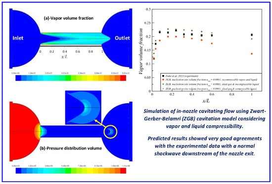
1. Introduction
Cavitation in confined flows is a highly complex phenomenon observed in many applications and can affect their performance considerably; the occurrence of cavitation in fuel supply systems of aircraft and automobiles, cryogenic pipelines and pipelines of nuclear power plants can lead to unexpected degradation in the system performance and damage to the components. The bubbly cavitating fluid behaves like a compressible fluid and has an unusual characteristic; the presence of even a small fraction of gas/vapor can considerably reduce the local sonic speed of liquid–gas mixture compared to the sonic speed within its constituents [1,2,3,4]. This unusual phenomenon occurs because the mixture phase is easily compressed owing to the compressibility of gas bubbles, however, it remains dense due to the dominant mass of the liquid [5]. Therefore, the bubbly flows in nozzles frequently become locally supersonic which leads to choking and the development of local shockwaves that impairs the performance [6]. Hence, because of the importance of an understanding of internal flows in nozzle design, several studies were conducted on flow inside the orifice which revealed complex bubbly flow behavior as described above. Typical nozzle geometries were sharp-edged entrance orifices [6,7,8], converging-diverging nozzles [9,10,11], and I-Channel [12]. Besides, many theoretical studies have been conducted to realize this phenomenon. Dorofeeva et al. [13] proposed a 1D barotropic model for cavitation prediction in the converging–diverging nozzle. The model assumed the fluid to be a homogenous mixture of liquid and cavitation vapor; the liquid was considered to be incompressible and the cavitation vapor to be an ideal gas. The model predicted a sharp rise in pressure or “shock” just downstream of the cavitation clouds where vapor transforms to liquid because of higher local pressure. The prediction of Battistoni et al. [14] also showed cavitation shock downstream of the cavitation cloud in a submerged nozzle. They used two different cavitation models with different multiphase modeling approaches to simulate the flow condition as described in [15]. The first cavitation model [16] was based on the homogeneous relaxation model (HRM) [17] and was used with Eulerian mixture model [18,19], the second cavitation model [20] was based on Rayleigh equation [21] and was used with Eulerian multi-fluid model [22]. The cavitation vapor was assumed to be an ideal gas, and the liquid was considered to be incompressible in both cases. Their comparison showed that the Rayleigh-Plesset equation-based cavitation model with Eulerian-Eulerian multi-fluid multi-phase model matched total void fraction more accurately than HRM cavitation model with Eulerian homogeneous equilibrium mixture model. However, they changed many variables at the time for the same operating condition. Hence reliable conclusions cannot be drawn from these comparisons. Cristofaro et al. [23] used I-Channel geometry as the test case for cavitation simulations with the objective of predicting cavitation erosion. For cavitation modeling, they used Grogger et al. [24] model with a sub-grid scale turbulence model based on coherent structures [25]. They assumed liquid to be compressible, but the vapor phase density was constant. They identified areas prone to erosion by the magnitude of predicted pressure peaks.
The objective of this work is to evaluate cavitation models for cavitating flows where compressibility plays a significant role. This study assesses two Rayleigh equation-based cavitation models to simulate the cavitating flow condition in the submerged orifice. The CFD simulations are evaluated by comparison of simulation results with the experimental data of Duke et al. [15] which contains both quantitative as well as qualitative information of void fraction, hence presents an excellent test case for CFD model evaluation. The models evaluated are SS [26] and ZGB [27] and according to the author’s knowledge, it is for the first time such simulations are evaluated assuming both phases to be compressible for the current nozzle geometry. The cavitation process is supposed to be isothermal, therefore, the liquid density is modeled using the Tait equation [28]. The Tait equation is a well-known EOS (equation of state) used to relate liquid density to pressure. It is an isentropic equation, based on two experimentally determined parameters. This equation has advantages that it can handle both high and very low pressures [29]. The vapor compressibility is modeled using the ideal gas law. The cavitation models are used with a multi-phase mixture model [18,19] which is recommended by [26] for cavitating flows. As per the present test case, the Reynolds number is around 15,800, the flow is wall-bounded and did not exhibit unsteadiness [15], thus, steady-state RANS (Reynolds Averaged Navier-Stokes) approach appeared to be the most desirable and consequently selected for this study due to its ability to predict such flows efficiently with sufficient accuracy [30]. The test case nozzle geometry was axis-symmetric which justifies our use of 2D axis-symmetric flow domain and mesh in which Navier-Stokes equations were solved in cylindrical form as this approach provides satisfactorily accurate results with the substantially lower computational cost and shorter computation time [31]. The turbulence models assessed are the Standard k-epsilon [32], Realizable k-epsilon [33], Launder and Sharma Low-Re k-epsilon [34], and SST k-omega [35].
Overall, the aim of the present work is to assess and analyze different cavitation and turbulence models quantitatively and qualitatively to select an appropriate model that can describe the cavitating flow within a nozzle accurately. Also, the outcome of this study is intended to help engineers and designers to further improve the designs of cavitating machines like fuel injectors and fuel supply systems of aircraft and automobiles by providing appropriate tools for calculating the cavitating flows accurately. The following section provides details of the flow geometry, which is followed by full details of the methodology. The results are presented and discussed in the subsequent section and the report ends with a summary of the main findings.
2. Flow Configuration
Duke et al. [15] performed X-ray radiography of a model single-hole nozzle to measure the cavitation vapor distribution. The test geometry was a polycarbonate nozzle with a throat diameter of D = 0.5 mm, a length/diameter ratio (L/D) of 5, and inlet to nozzle diameter ratio of 5 as shown in Figure 1. The working fluid was commercial surrogate gasoline with a density equal to 777.97 , the viscosity of 8.48 and the vapor pressure of 580 at 25 °C. The working fluid was delivered via a piston accumulator system pressurized with an inert gas. The fluid temperature and pressure were monitored immediately upstream, and downstream of the nozzle and a turbine flow meter was used to monitor the flow rate. The injection pressure and back pressure were varied independently to obtain the desired flow rate. Operating condition of the experiment is listed in Table 1, and the same operating condition was used for the CFD simulations in this study.
During the X-ray radiography experiment, the 7-BM beamline of the advanced photon source was with the focused beam acting as a microprobe, allowing the void fraction to be probed on the small area along the line of sight. They passed the nozzle through the fixed beam in a raster pattern at 100 transverse positions (y) and 19 streamwise positions (x), the raster scan grid can be seen in Figure 2a. The time-averaged values were interpolated onto a series of contour plots, as shown in Figure 2b which shows cavitation originating near the sharp entrance of the nozzle. At half of the nozzle length, the vapor layer attached to the wall begins to collapse while a considerable void cloud was recorded at the core of the nozzle which then extends to the nozzle outlet. It was argued [15] that the presence of void at the centerline is more likely due to convection of vapor from the wall because of negatively inward pressure gradient than due to isolated nucleation events as described by Bauer et al. [36]. Nonetheless, the time-averaged measurements of vapor quantity achieved an uncertainty of 2% implying a steady flow regime. Duke [15] has also performed imaging using conventional X-ray, the result of which is shown in Figure 2c which is a time-averaged X-ray image of the nozzle inlet which also described the above-stated phenomenon. For more details about the experimental work, please refer to the original work [15].
3. Methodology
3.1. Mixture Model
The mixture model solves one set of conservation equation for mass, momentum, and energy and the volume fraction equation for the second phase with the addition of the turbulence closure model. The model assumes that velocity, temperature, and pressure between the phases are equal. This assumption is based on the idea that the difference between three potential variables would facilitate mass, momentum, and energy transfer between phases so fast that equilibrium would be achieved within an extremely small time scale (almost instantly). Therefore, the resulting equations resemble a pseudo-fluid with mixture properties and the equation of state which links phases, so mixture thermodynamics properties are obtained [18,19].
The steady-state version of the model equations are presented here. The following formulation is used to calculate mixture density:
where is the volume fraction of the phase . Since in the present study, the multiphase system is comprised of two phases, hence, the mixture density is computed using the following equation:
Since,
Hence, Equation (2) becomes:
Similarly, the viscosity of the mixture can also be calculated as:
where is the molecular viscosity of liquid and is the molecular viscosity of the vapor.
3.2. Cavitation Models
3.2.1. Schnerr and Sauer (SS) Model
The SS model [23] treats the bubbly flow as a homogeneous vapor-liquid mixture. The model assumes the vapor phase to consist of numerous mini spherical bubbles. The model uses the Rayleigh relation [21] for the description of bubble growth and collapse.
where is the radius of the bubble, is the saturation vapor pressure, and is the far-field pressure, however for the practical purpose is taken to be the same cell center pressure [26].
The model defines the vapor volume fraction using the following equation:
where is defined as the bubble number density per unit volume of pure liquid. Using Equation (8), the following equation is derived for the bubble radius:
The transport equation for the vapor fraction is:
where is the net phase change rate.
The phase transfer rate terms are as follows:
When , evaporation (cavitation)
When , condensation
The vapor volume fraction is dependent on the which is a constant and assuming no change in the nucleation site per unit volume of pure liquid. The originally recommended value of is which is used in this study in initial simulations, voften is required to be adjusted to match the experimental data as shown by Yuan et al. [37].
3.2.2. Zwart, Gerber, and Belamri (ZGB)
The ZGB model [27] also assumes the fluid to be a homogeneous liquid–vapor mixture, and the model similarly assumes vapor to consist of tiny spherical bubbles. The ZGB model also uses the Rayleigh relation (Equation (8) for the description of bubbles growth and collapse in vapor production (cavitation) and destruction (condensation) terms [27]. The following equation defines the vapor volume fraction:
where is again the bubble radius, is the bubble concentration per unit volume of the fluid mixture. The transport equation for the vapor fraction is formerly identical to the SS model as:
where R is again the net phase change rate and is defined using the following equation:
The phase transfer rate terms are as follows:
When , evaporation
When , condensation
Zwart et al. [27] reported that the model works well for condensation but produces physically incorrect results (and numerically unstable) when employed for cavitation. This is because the model assumes no interaction between the cavitation bubbles, which is only possible in the early stages of cavitation when cavitation bubbles grow from a nucleation site. However, they argued that when the vapor volume increases, the nucleation site density must decrease accordingly. Hence, Zwart et al. proposed to replace with in the evaporation term , where is the nucleation site volume fraction. Hence, final forms of rate equations are:
When , evaporation
When , condensation
The values of model constants are, , and .
3.3. Liquid and Vapor Compressibility Models
3.3.1. Tait Equation
Tait establishes a nonlinear relationship between the density of the liquid and its pressure under isothermal conditions. The Tait equation can be expressed in terms of pressure and density using the following relationship:
where and are coefficients which can be defined by assuming that bulk modulus is a linear function of pressure, the values of and are based on the reference state values of pressure, density, and bulk modulus. is known as density exponent, having a similar role as a ratio of specific heats [38].
The simplified Tait equation as implemented in the ANSYS Fluent platform has the following form [39]:
where
and
where is the reference liquid pressure, is the reference liquid density which is the density at the reference pressure , is density exponent, for which the value 7.15 is used which corresponds to weakly compressible materials such as liquids [38], is the reference bulk modulus at the reference pressure , is the liquid pressure (absolute), is the liquid density at the pressure , and is the bulk modulus at the pressure . The reference values that are considered in this study are of gasoline at the average temperature of 25 °C [40] and listed in Table 2.
The speed of sound in the liquid phase is calculated using the following equation:
3.3.2. Ideal Gas Law
The vapor density is modeled using the ideal gas law which has the following form:
where is the universal gas constant, is the molecular weight, and is the temperature. The speed of sound in the gas phase is calculated using the following equation:
where is the specific heat ratio, and it is defined by the following equation:
where is the specific gas constant , is the specific heat capacity at the constant pressure, and is the specific heat capacity at the constant volume.
3.4. Sonic Speed in Mixture Phase Model
Wallis Sonic Speed in the Two-Phase System
The speed of sound in the mixture phase is computed using the Wallis Model [41], the model assumes local thermodynamic equilibrium between phases and has been implemented in the following form in ANSYS Fluent [42]:
where is the speed of sound in the liquid–vapor mixture. The readers can find the complete derivation of Equation (29) in [43].
4. Numerical Methods
The governing equations are solved using commercial CFD solver ANSYS Fluent v14.5 which uses the finite volume method [30]. Acknowledging that the flow regime is steady [15], steady-state simulations have been performed, and for pressure-velocity coupling, the SIMPLE algorithm is employed. Since the nozzle geometry is axis-symmetrical, a 2D axis-symmetrical flow domain (as shown in Figure 3) has been chosen for the CFD simulations and cylindrical form of governing equations (Equations (6), (7), and (11)) are solved. The 2D grid contained quad type elements. The operating boundary conditions used to simulate the flow are the same as those used in the experiment as specified in Table 1. The grids of the main flow region (the red box shown in Figure 3) were locally refined as shown in Figure 4. The influence of the number of cells in grids was checked by comparing predicted vapor volume fraction and velocity as shown in Figure 5a,b, respectively. The first grid comprised 89,189 cells or an approximate average cell size of 16.87 microns, the second grid contained 121,526 cells and hence had an average cell size of about 14.45 microns, and the third grid had 273,563 cells with average cell size was approx.10.06 microns. The cell ratio between the first grid and the second grid was 1.16 and between the second and third grid was 1.43. The authors achieved a good compromise between second and third grids in terms of results of mean axial velocity and vapor volume fraction, as shown in Figure 5. However, after the third refinement, the authors did not achieve y+ < 1 which is required to run low-Re turbulence models [30]. Hence grids were refined only in the near-wall region to ensure y+ < 1 was achieved. Hence, there is not much difference between the third grid and the final grid in terms of the cell quantity.
In the grid independence test high Reynolds number standard k-epsilon model [32] was used, and near-wall turbulence was simulated using the EWT (enhanced wall treatment method), which is a near-wall modeling approach that blends linear (laminar) and logarithmic (turbulent) laws-of-the-wall using a joining function [44]. For cavitation modeling, the ZGB cavitation model has been used with a mixture multiphase model. The operating condition and physical properties of the working fluid are listed in Table 1 and Table 2. The effect of convergence was checked by changing the convergence criteria of continuity, momentum, k, and epsilon from 1 × 10⁻⁴ to 1 × 10⁻⁶ which showed no observable changes on the solution.
5. Results and Discussion
5.1. Influence of Turbulence Modelling
In this section, impacts of four different turbulence models on cavitation vapor predictions are assessed. Turbulence models evaluated here are the Standard k-epsilon, Realizable k-epsilon, Launder and Sharma k-epsilon, and SST k-omega. The density of both vapor and liquid phases are assumed to be constant. This assumption is only justified if the volume fraction is low [4], but has advantages as it allows the volume fraction transport equation (see Equations (10) and (15)) to become just a volume conservation equation. Thus it helps solutions to become more numerically stable, and therefore enables researchers to assess models in the early stages of assessments, and hence, it has been used by many researchers like [27,39,45,46,47]. Rigorous evaluations were carried out to select an appropriate turbulence model for this study with full details given by [48], and a summary of some of these simulation tests with comparison to experimental data is given below in Figure 6 and Figure 7.
The total quantity of vapor integrated over the nozzle cross-section at different axial locations (x/L) for different models has been compared with experiment and is represented in Figure 6. Before discussing the quantitative comparison, it would be useful to know how the vapor is distributed within the nozzle. Observing the experimental X-ray radiography image, Figure 7a, shows that vapor is generated at the sharp entrance of the nozzle orifice, as expected. The vapor then disperses from near the wall and mixes with the flow as it travels further downstream. Also, the accumulation of vapor along the nozzle axis downstream of the entrance can be seen clearly. It was argued [15] that the observed asymmetric vapor distribution has been attributed to small machining defects which may have provided additional nucleation sites to the nozzle.
On comparison of the predicted results using for different turbulence models shown in Figure 6, it is clear that the realizable k-epsilon and standard k-epsilon models outperformed the other two models, and that the realizable k-epsilon model predictions give closer agreement with the experimental data than the standard k-epsilon model, especially toward the exit of the nozzle. The results show the realizable k-epsilon model overpredicts the vapor fraction near the entrance and becomes similar as x/L increases, while the standard k-epsilon model underpredicts in the beginning of the nozzle and the difference becomes much wider with downstream distance. This can be correlated with the larger recirculation zone predicted using the realizable k-epsilon model at the beginning of the nozzle (x/L = 0.0167) as shown fully in [48] from the mean axial velocity profiles; the larger recirculation zone corresponds to higher flow acceleration into the nozzle, which in turn reduces the pressure more (or more saturated pressure as shown in [48]), and hence more cavitation leading to the larger prediction of vapor volume.
In addition, the qualitative comparison of the vapor fraction predictions with experiment, Figure 7, confirms the conclusion made in Figure 6 that the realizable k-epsilon and standard k-epsilon models outperform the other two models; the graphs for other two models are not plotted here but can be found in [48]. However, the conclusion drawn between the realizable k-epsilon and standard k-epsilon models is not as clear as that of Figure 6. The comparison of the results in Figure 7a–c, indicate a slightly better agreement between the experiment and the standard k epsilon model than the realizable k epsilon model. The CFD results suggest that vapor is generated at the sharp entrance of the nozzle orifice for both models. However, the generated vapor with the standard k-epsilon models is dispersing from the vicinity of the wall toward axis and mixing with the liquid as the flow is converted downstream, but the cavitation structure disappears at the orifice exit, Figure 7b. Although similar dispersion of the vapor can be seen with realizable k-epsilon model, the vapor never reaches the nozzle axis, and that the cavitation structure extends beyond the exit of the nozzle, Figure 7c. These features are further confirmed when the cavitation contours for both models are plotted outside the orifice by [48], where the results clearly show the extension of cavitation into the circular expansion region of the orifice for the realizable k-epsilon model, while it terminates at the exit of the orifice for the standard k-epsilon model. It is also clear from Figure 7 that the intensity of the cavitation is higher with the realizable k-epsilon model in line with the results obtained in Figure 6.
The observed difference in the behavior of standard k-epsilon and realizable k-epsilon models can be attributed to the turbulent variable used in the realizable k-epsilon model while it is treated as a constant in the standard k-epsilon model. Further analysis made by Kumar [48] showed clearly that the had a direct influence on the turbulent viscosity and the whole flow field so that a lower turbulent viscosity is predicted using the realizable k-epsilon model than the standard k-epsilon. Therefore, the predicted larger recirculation region, mentioned above, with the realizable k-epsilon at the orifice entrance can be attributed to the lower turbulent viscosity that resulted in more saturated pressure region, and thus more intense cavitation. On the other hand, the higher turbulent viscosity predicted with the standard k-epsilon model has resulted in more diffusion between phases, see Figure 7a,b. Therefore, from these analyses, it can be stated that the different turbulent viscosity formulation in the realizable k-epsilon model has resulted in a more accurate prediction of the recirculation region and flow reattachment and led to a more accurate prediction of vapor volume fraction in the present case.
In general, the full analysis given in [48] showed that the volume fraction has been underpredicted using the Launder and Sharma low-Re k-epsilon turbulence model because it has the same transport equations as the standard k-epsilon model, as well as the same turbulent viscosity formulation. However, this model has additional source terms in the transport equations for k-epsilon as well as damping functions that are active only close to the wall allowing the model to predict k-epsilon in the viscous sublayer, hence, the model does not use wall functions. Nevertheless, the results indicate that the model’s low-Re approach has failed to completely capture the flow regime for the present case. The model has predicted a smaller recirculation region at the axial position x/L = 0.0167 near the entrance of the nozzle, which resulted in the smaller low-pressure region and therefore lesser cavitation; the analysis also showed that as the fluid moves downstream the cavitation is largely seen to stay in the vicinity of the wall and collapses well before the nozzle exit; around two-third of the orifice length.
The SST k-omega model uses features of the standard k-epsilon in the far-field region and the standard k-omega model [30] in the near-wall region; the k-omega terms are integrated throughout the viscous sublayer hence the model does not require wall functions. In addition, the model also has a different formulation for turbulent viscosity than the k-epsilon family of models. The model, in general, well overpredicts the generation of vapor, Figure 6, but the vapor tends to remain in the vicinity of the wall as fluid moves downstream and enters the circular expansion region of the nozzle. On comparing the mean axial velocity profiles, at x/L = 0.0167, it formed the largest recirculation region (compare to other three models) leading to the largest vapor prediction, Figure 6. However, the cavitation with this model did not diffuse and mixes with liquid like other three cases and remained close to the wall, which can be attributed to different turbulent viscosity formulation in the SST k-omega model that give very low turbulent viscosity leading to lower diffusion. Overall, the performed analysis concludes that the realizable k-epsilon model gave the best overall results for the present case, therefore it is chosen in the present study in later simulations. Readers might refer to [48] to gain more information about the above simulation and analysis on the selection of turbulence model for this study.
5.2. Cavitation Model Assessment
As mentioned before, two cavitation models have been assessed, the SS model and the ZGM model. The models are analyzed quantitatively and qualitatively by comparing the predicted results with the experimental data. The quantitative comparison of predicted results with experimental measurements of [15] is presented in Figure 8 and shows the total volume fraction of vapor along the nozzle axis. The comparison indicates that the SS model gives a good agreement with experimental data up to = 0.6 with a difference of up to 7%, while the ZGB model predicts a higher vapor volume within the same range with differences up to 20%. Both models underpredict the volume faction at the exit, in particular, the SS models. This will be explained later when considering the assessment of evaporation and condensation of the two models.
To obtain a better understanding of vapor fraction distribution within the nozzle, the qualitative spatial comparison of the predicted vapor fraction contours for both models with X-ray radiography measurements is made and are shown in Figure 9a–c, which suggests that both models have failed to capture the flow features adequately in the core of the nozzle along the axis, in particular at the downstream near the exit where the experimental results show considerable void while they are absent in both model predictions. This can be better realized by the results of both models presented in Figure 10a,b, where they show that the cavitation initiates at the sharp entrance of the orifice after which it converts downstream with the liquid. Both models predict that the significant proportion of vapor remains near the wall with the uniform annular expansion with downstream distance (x/L) so that at the exit, the vapor bubbles cover almost 2/3 of the diameter. After the exit, the vapor bubbles start to reduce considerably so that they are diminished at distances 1.0D and 0.5D downstream of the exit for the SS and ZGB model, respectively; the reason for this is the vapor transforms back to liquid because of higher pressure within the circular expansion region. As aforementioned, both models have failed to predict vapor along the centerline as found in experimental results.
To further analyze the predictions, it was decided to plot and compare the evaporation and condensation rate terms of both models. It should be noted that the evaporation and condensation rates in the SS model is non-linear and is proportional to and has an unusual property; it approaches zero when and and is maximum in between. Hence, the SS model requires a particular value of vapor fraction at the inlet boundary to initiate cavitation. The value used in the present case for the SS model is as recommended by [26], which is not the case for the ZGB model. The vaporization and condensation rates in the ZGB model are linear and start from the initial value.
Hence, the ratio of evaporation and condensation rates of both models for the range of is plotted and is shown in Figure 11a,b. The evaporation rate graph in Figure 11a shows that the evaporation rate of the ZGB model is higher than that of the SS model in the range of after which it becomes smaller than the SS model. The condensation rate ratio graph in Figure 11b also suggests a higher condensation rate for ZGB model in a much small range, i.e., , following which the condensation rate is greater in the SS model in the remaining of the range. From this comparison, it can be stated that the higher vapor volume fraction predicted in the ZGB model was because of the higher initial evaporation rate in the ZGB model over the SS model and lesser overall condensation rate of ZGB model.
This study also assesses the influence of model constants on cavitation results associated with liquid quality. One of the essential factors that affect the liquid quality is the bubble nuclei population. In real liquids, nuclei may comprise small gas bubbles and impurities [47]. Brennen [4] explained that the bubble nuclei of larger than critical value could assist cavitation more substantially while smaller ones would stay in the liquid. Both models contain constants that need to be adjusted to account for the liquid quality. One such constant in the SS model is , which expresses the bubble concentration per unit volume of pure liquid. The ZGB model also contains many constants such as bubble radius , nucleation site volume fraction , and that need tuning for optimum physical results.
In the initial simulations, the SS model constant was varied and ZGB model constant is adjusted. The results presented in Figure 12 indicate that the cavitation vapor volume in these models can be adjusted by changing model constants. The SS model gave the best result when the value of the model constant is The ZGB model slightly overpredicts the vapor volume when the value of the model constant is set to 0.0005 however, when is set to 0.0001, the model to some extent underpredicts the same. The ZGB model contains other empirical tunable constants such as , and which are scalars and can be adjusted to allow users to further optimize predictions. However, the impacts of varying these constants are not considered here to avoid reader divergence since changing these constants leads to many permutations and combinations leading the present investigation to become merely a curve-fitting exercise. Also, in the above simulations, both phases are considered incompressible which is not physically accurate [4]. Therefore, it is necessary to evaluate both models by considering both phases to be compressible as described in the next section.
5.3. Influence of Compressibility
The liquid compressibility is modeled using the Tait equation (Equation (21)), and the ideal gas law (Equation (25)) is applied to model the vapor compressibility. The speed of sound in the bubbly phase is modeled using the Wallis equation (Equation (28)). Figure 13 shows the influences of vapor compressibility by comparing the predicted vapor faction from different models with the experimental. It is evident that the inclusion of the vapor compressibility makes significant improvement and predicts a closer vapor distribution to that of the experimental data, Figure 13a,c,e. However, when the vapor was assumed to be an ideal gas, the results obtained from a fully converged solution using the SS model were non-physical and deviated significantly from experimental results particularly in the core region of the flow as shown in Figure 13c. This is mainly believed to be due to the overprediction of condensation rate (as previously shown in Figure 11). Therefore, the SS model was abandoned at this stage, and that the results obtained using only the ZGB model are considered for further analysis in this study.
The quantitative comparison of predicted vapor volume fraction using the ZGB model presented in Figure 14 clearly shows an increase in the vapor volume fraction when vapor is assumed to be the ideal gas. This is because the ideal gas assumption allowed the vapor volume to change with the change in the local pressure. Therefore, the vapor volume expanded and its density decreased as the pressure decreased. The comparison also shows better agreements achieved with the experimental data when using the ideal gas assumption for cavitation vapor. In addition, another simulation with the liquid compressibility was modeled using the Tait equation and the results are superimposed in Figure 14, which clearly show that the liquid compressibility assumption made no difference in the cavitation results, implying that liquid compressibility has an insignificant impact in this case as expected for an upstream-downstream pressure ratio of 10 bars [4]. In this case study, during the assessment of the SS model, the value of was increased by a factor of ten from to . The results of = are only presented as the results for a subsequent increase in did not show any significant physical changes and improvements. While assessing the ZGB model, was set equal to 0.0001 and was not further changed as it provided fairly good agreement with experimental measurements and with the vapor compressibility model (ideal gas law). The other model constants were not changed.
As was shown in Figure 13, the qualitative comparison of predicted vapor fraction with experimental measurements, presented in Figure 13a,e, clearly indicates a much better agreement when vapor is assumed to be an ideal gas than incompressible, Figure 13d, and therefore has been adopted to simulate the flow. Prediction results using the ideal gas model for vapor compressibility over the whole flow domain shows that the vapor generates at the sharp entrance of the nozzle orifice. As the fluid travels further downstream, the vapor separates from the wall and moves toward the nozzle center as it mixes with the liquid flow and reaches the nozzle axis (centerline) at around 2.5 diameters downstream of the nozzle entrance as it can be seen in Figure 15a. When the vapor is assumed to be incompressible, the predicted vapor contours are similar to the previous results presented in Figure 9c with no presence of cavitation around the center of the nozzle.
Moreover, on further examining the flow field of numerical simulation, in which vapor assumed as the ideal gas and liquid density modeled using the Tait equation, the vapor volume fraction contours in Figure 15a shows that after the nozzle exit the vapor fraction diminishes radially with downstream distance so that all vapor transforms into a liquid at a distance away from the exit on the centreline. At the same position () the pressure contours in Figure 15b show a sudden surge in pressure (up to 3.7 bars), which can be seen more clearly on the inserted zoomed picture of the radial pressure distribution. This sudden sharp pressure rise downstream of the nozzle exit can also be seen clearly in Figure 16a at the same location where the pressure profile on-axis shows a sudden rise with a correspondence sharp drop in velocity at the same location as shown in Figure 16b. These sharp rise and fall in pressure and velocity, respectively, in bubbly flows are usually associated with the presence of a normal shock wave [18].
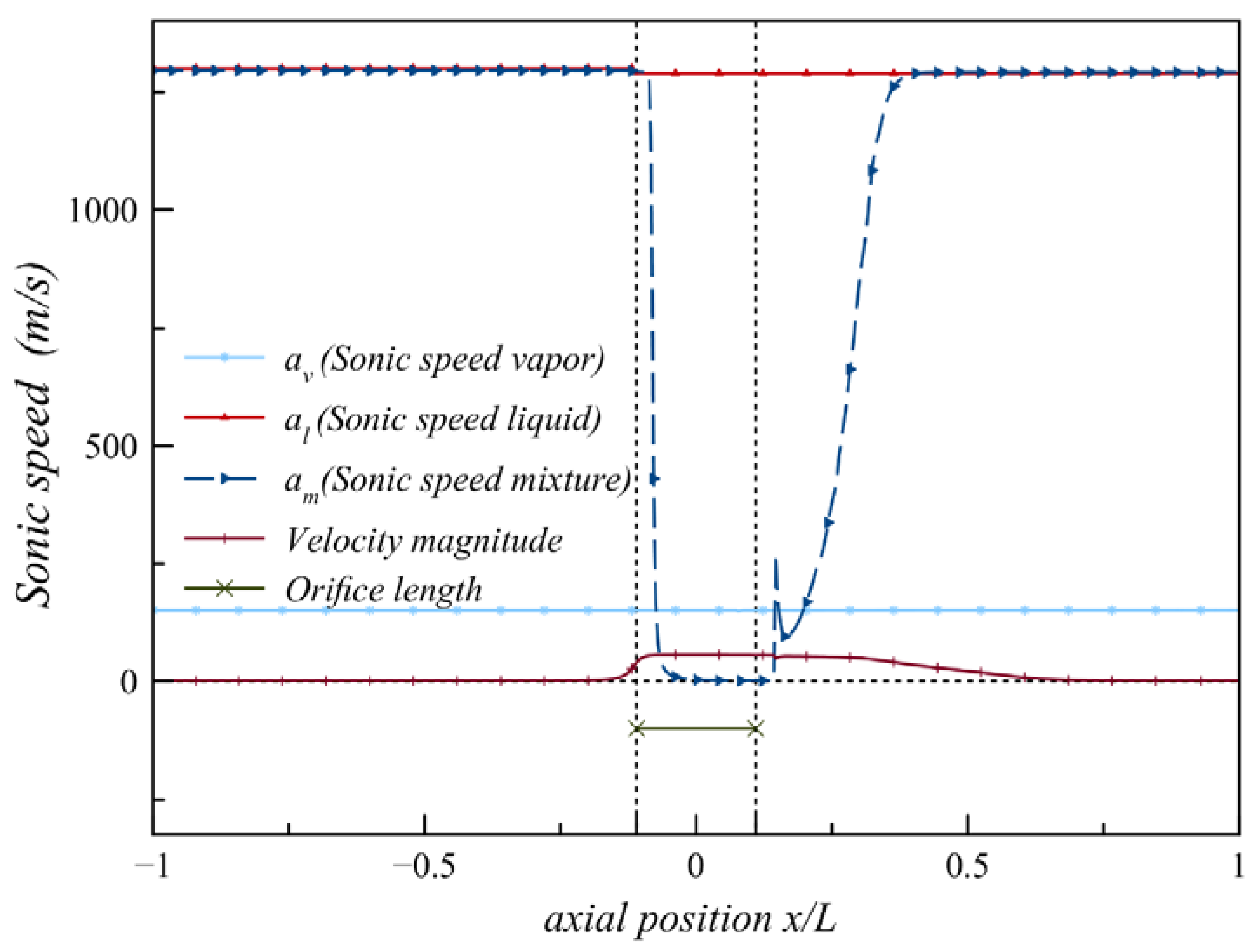
To further investigate the formation of the shockwave, local sonic speeds in the liquid phase, , the vapor phase, , and the mixture phase (cavitation region), and the flow velocity magnitude on the nozzle axis are plotted in Figure 17, which show that local sonic speed in the mixture phase is substantially reduced and becomes significantly smaller than the flow velocity within the nozzle orifice region ) and up to a distance from the nozzle exit. Figure 17 also indicates that local sonic speed in the mixture phase becomes considerably lower than local sonic speeds of vapor and liquid phases, implying that the local flow in the mixture phase becomes supersonic in the cavitation region. Downstream of the cavitation region at (or 1.63 mm), the fluid transforms back to the liquid state because of the higher local pressure (Figure 15b and Figure 16a). Thus, the local flow becomes subsonic from supersonic and hence, as a consequence, a normal shockwave is formed.
6. Conclusions
A cavitating flow in a submerged orifice was used to evaluate the predictive capability of different cavitation models for compressible flows. The current flow geometry in a single nozzle has been chosen because there was useful detailed experimental data, which were used to assess the models. The performance of different turbulence models was also evaluated for the same flow geometry. The simulation results were compared with experimental data for validation of models and selection of an appropriate model to evaluate the cavitating flow accurately. The following are a summary of the main findings and contributions of the current research study:
- Four turbulence models were evaluated, the standard k-epsilon, realizable k-epsilon, Launder and Sharma k-epsilon, and SST k-omega. The results showed that turbulent viscosity profoundly affected the results, and that the realizable k-epsilon model was found to provide the most accurate results which is believed to be due to the formulation of turbulent viscosity.
- The performance of the SS and ZGB cavitating models were analyzed and compared. The comparison of results showed higher vapor volume fraction when using the ZGB model because of the higher initial evaporation rate in the ZGB model, and lesser overall condensation rate with the ZGB model. The analyses also suggested that using incompressible liquid and vapor assumption, the models failed to capture the flow physics accurately.
- Simulations of the models with both liquid and vapor phase to be compressible showed that the SS model failed to predict the flow physics with a weak agreement with experimental data particularly in the nozzle core region, which is again believed to be due to the overestimation of condensation rate. However, the prediction results of the ZGB model were in better agreement with the experimental data and showed the ideal gas assumption allowed the cavitation vapor volume to change by the change in the local pressure. As a result, the cavitation vapor volume has been improved and increased compared to the incompressible assumption, particularly on the core region. In addition, a normal shockwave was predicted downstream of the cavitation region where the local sonic speed becomes subsonic from supersonic.
Overall, the chosen ZGB cavitation model with inclusion of the compressibility provided very good agreements with the experimental data across the nozzle particularly in the core of the nozzle along the axis and outside the nozzle exit. The outcome of this study will provide appropriate tools for engineers to further improve the calculation of cavitating flows and the designs of the related machines.
Author Contributions
Methodology, A.K.; Formal analysis, A.K.; Writing—Original Draft, A.K.; Writing—Review & Editing, A.K., A.G. and J.M.N.; Conceptualization, A.G.; Supervision, A.G. and J.M.N.; Funding acquisition, J.M.N. All authors have read and agreed to the published version of the manuscript.
Funding
This research received no external funding. However, full studentship financial support has been received from City, University of London.
Acknowledgments
The authors would like to thank the financial support from the School of Mathematics, Computer Sciences, and Engineering, City, University of London. The authors would also like to appreciate the help provided by Chris Marshall for using the university cluster. Finally, our special thanks to Yvette Woell from Argonne National Laboratory, Lemont, Illinois, USA for granting permission to reproduce images from the article “Synchrotron X-Ray Measurements of Cavitation” for this paper.
Conflicts of Interest
The authors declare that there is no conflict of interest.
Nomenclature
| speed of sound in the liquid phase | |
| speed of sound in the liquid-vapor mixture | |
| speed of sound in the vapor phase | |
| specific heat at constant pressure | |
| specific heat at constant volume | |
| cavitation number | |
| Nozzle diameter | |
| condensation coefficient | |
| evaporation coefficient | |
| reference bulk modulus | |
| bulk modulus | |
| L | Length of the nozzle |
| molecular weight | |
| density exponent | |
| bubble number density per unit volume of pure liquid | |
| bubble number density per unit volume of fluid mixture | |
| reference pressure | |
| pressure | |
| far-field pressure | |
| saturated vapor pressure | |
| saturation vapor pressure | |
| bubble radius | |
| bubble growth rate | |
| specific gas constant | |
| net phase change rate | |
| net condensation rate | |
| net evaporation rate | |
| universal gas constant | |
| Reynolds Number | |
| Temperature |
Greek Symbols
| liquid volume fraction | |
| vapor volume fraction | |
| nucleation site per volume fraction | |
| specific heat ratio | |
| molecular viscosity of the mixture | |
| molecular viscosity of the liquid | |
| molecular viscosity of the vapor | |
| reference density of liquid | |
| density of mixture | |
| density of the liquid | |
| density of the vapor | |
| mixture shear stress tensor |
References
- Karplus, H.B. Velocity of sound in a liquid containing gas bubbles. J. Acoust. Soc. Am. 1957, 29, 1261–1262. [Google Scholar] [CrossRef]
- Semenov, N.I.; Kosterin, S.I. Results of studying the speed of sound in moving gas-liquid systems. Teploenergetika 1964, 11, 46–51. [Google Scholar]
- Henry, R.E.; Grolmes, M.A.; Fauske, H.K. Pressure-Pulse Propagation in Two-Phase One-and Two-Component Mixtures. Technical Report No. ANL-7792; Argonne National Lab., Ill: Lemont, IL, USA, 1971. [Google Scholar] [CrossRef] [Green Version]
- Brennen, C.E. Cavitation and Bubble Dynamics; Oxford University Press: New York, NY, USA, 1995; Volume 44. [Google Scholar]
- McWilliam, D.; Duggins, R.K. Speed of sound in bubbly liquids. Inst. Mech. Eng. Conf. Proc. 1969, 184, 102–107. [Google Scholar] [CrossRef]
- Soteriou, C.; Andrews, R.; Smith, M. Direct Injection Diesel Sprays and the Effect of Cavitation and Hydraulic Flip on Atomization. SAE Trans. 1995, 104, 128–153. [Google Scholar]
- Numachi, F.; Yamabe, M.; Oba, R. Cavitation Effect on the Discharge Coefficient of the Sharp-Edged Orifice Plate. ASME J. Basic Eng. 1960, 82, 1–6. [Google Scholar] [CrossRef]
- Yan, Y.; Thorpe, R.B. Flow regime transitions due to cavitation in the flow through an orifice. Int. J. Multiph. Flow 1990, 16, 1023–1045. [Google Scholar] [CrossRef]
- Simoneau, R.J. Pressure distribution in a converging-diverging nozzle during two-phase choked flow of subcooled nitrogen. In Proceedings of the Winter Animal Meeting of the American Society of Mechanical Engineers, Houston, TX, USA, 30 November–5 December 1975. Nasa Technical Report, 75N26306, Full Text. [Google Scholar]
- Simoneau, R.J.; Hendricks, R.C. Two-phase choked flow of cryogenic fluids in converging-diverging nozzles. NASA STI/Recon Tech. Rep. N 1979, 79, 29468. [Google Scholar]
- Waldrop, M.; Thomas, F. Video: Shock wave propagation: Cavitation of dodecane in a converging-diverging nozzle. In Proceedings of the 68th Annual meeting of APS Phys, Boston, MA, USA, 22–24 November 2015. [Google Scholar] [CrossRef]
- Winklhofer, E.; Kull, E.; Kelz, E.; Morozov, A. Comprehensive hydraulic and flow field documentation in model throttle experiments under cavitation conditions. In Proceedings of the ILASS-Europe 2001, 17 International Conference on Liquid Atomization and Spray Systems, Zurich, Switzerland, 2–6 September 2001. [Google Scholar] [CrossRef]
- Dorofeeva, I.; Thomas, F.; Dunn, P. Cavitation of JP-8 fuel in a converging-diverging nozzle: Experiments and modeling. In Proceedings of the 7th International Symposium on Cavitation, Ann Arbor, MI, USA, 17–22 August 2009. [Google Scholar]
- Battistoni, M.; Som, S.; Longman, D.E. Comparison of mixture and multifluid models for in-nozzle cavitation prediction. J. Eng. Gas Turbines Power 2014, 136, 61506. [Google Scholar] [CrossRef]
- Duke, D.; Kastengren, A.; Tilocco, F.Z.; Powell, C. Synchrotron x-ray measurements of cavitation. In Proceedings of the 25th Annual Conference on Liquid Atomization and Spray Systems, ILASS-Americas, Pittsburgh, PA, USA, 21–23 May 2013; pp. 5–8. [Google Scholar]
- Schmidt, D.P.; Gopalakrishnan, S.; Jasak, H. Multi-dimensional simulation of thermal non-equilibrium channel flow. Int. J. Multiph. Flow 2010, 36, 284–292. [Google Scholar] [CrossRef]
- Bilicki, Z.; Kestin, J. Physical aspects of the relaxation model in two-phase flow. R. Soc. London A Math. Phys. Eng. Sci. 1990, 428, 379–397. [Google Scholar]
- Brennen, C.E. Fundamentals of Multiphase Flow; Cambridge University Press: Cambridge, UK, 2005. [Google Scholar]
- Manninen, M.; Taivassalo, V.; Kallio, S. On the Mixture Model for Multiphase Flow; VTT Publications 288: Espoo, Finland, 1996. [Google Scholar]
- Battistoni, M.; Grimaldi, C.N. Analysis of transient cavitating flows in diesel injectors using diesel and biodiesel fuels. SAE Int. J. Fuels Lubr. 2010, 3, 2010-01-2245. [Google Scholar] [CrossRef]
- Rayleigh, L., VIII. On the pressure developed in a liquid during the collapse of a spherical cavity. London, Edinburgh, Dublin Philos. Mag. J. Sci. 1917, 34, 94–98. [Google Scholar] [CrossRef]
- Drew, D.A.; Passman, S.L. Theory of Multicomponent Fluids; Springer Science & Business Media: Berlin/Heidelberg, Germany, 2006; Volume 135. [Google Scholar]
- Cristofaro, M.; Edelbauer, W.; Koukouvinis, P.; Gavaises, M. Influence of Diesel Fuel Viscosity on Cavitating Throttle Flow Simulations under Erosive Operation Conditions. ACS Omega 2020, 5, 7182–7192. [Google Scholar] [CrossRef] [PubMed]
- Grogger, H.A.; Alajbegovic, A. Calculation of the cavitating flow in venturi geometries using two-fluid model. In Proceedings of the SME Proceeding, FEDSM’98, Washington, DC, USA, 21–25 June 1998; p. 5295. [Google Scholar]
- Kobayashi, H. The subgrid-scale models based on coherent structures for rotating homogeneous turbulence and turbulent channel flow. Phys. Fluids 2005, 17, 45104. [Google Scholar] [CrossRef]
- Schnerr, G.H.; Sauer, J. Physical and numerical modelling of unsteady cavitation dynamics. In Proceedings of the 4th International Conference on Multiphase Flow, New Orleans, LA, USA, 27 May–1 June 2001; Volume 1. [Google Scholar]
- Zwart, P.J.; Gerber, A.G.; Belamri, T. A two-phase flow model for predicting cavitation dynamics. In Proceedings of the 5th International Conference on Multiphase Flow, Yokohama, Japan, 30 May–4 June 2004. [Google Scholar]
- Dymond, J.H.; Malhotra, R. The Tait equation: 100 years on. Int. J. Thermophys. 1988, 9, 941–951. [Google Scholar] [CrossRef]
- Koukouvinis, P.; Gavaises, M.; Li, J.; Wang, L. Large Eddy Simulation of Diesel injector including cavitation effects and correlation to erosion damage. Fuel 2016, 175, 26–39. [Google Scholar] [CrossRef] [Green Version]
- Wilcox, D.C. Turbulence Modeling for CFD; DCW Industries: La Canada, CA, USA, 1998; Volume 2. [Google Scholar]
- Irawan, D.; García, A.; Gutiérrez, A.J.; Álvarez, E.; Blanco, E. Modeling of coil cooling using 2D and 3D computational fluid dynamics (CFD). In Proceedings of the 3rd International Congress on Water, Waste and Energy Management, Rome, Italy, 18–20 July 2016. [Google Scholar]
- Jones, W.P.; Launder, B.E. The prediction of laminarization with a two-equation model of turbulence. Int. J. Heat Mass Transf. 1972, 15, 301–314. [Google Scholar] [CrossRef]
- Shih, T.H.; Liou, W.W.; Shabbir, A.; Yang, Z.; Zhu, J. A new k-epsilon eddy viscosity model for high Reynolds number turbulent flows: Model development and validation. ScienceDirect 1995, 24, 227–238. [Google Scholar]
- Launder, B.E.; Sharma, B.I. Application of the energy-dissipation model of turbulence to the calculation of flow near a spinning disc. Lett. Heat Mass Transf. 1974, 1, 131–137. [Google Scholar] [CrossRef]
- Menter, F.R. Two-equation eddy-viscosity turbulence models for engineering applications. AIAA J. 1994, 32, 1598–1605. [Google Scholar] [CrossRef] [Green Version]
- Bauer, D.; Chaves, H.; Arcoumanis, C. Measurements of void fraction distribution in cavitating pipe flow using x-ray CT. Meas. Sci. Technol. 2012, 23, 55302. [Google Scholar] [CrossRef] [Green Version]
- Yuan, W.; Sauer, J.; Schnerr, G.H. Modeling and computation of unsteady cavitation flows in injection nozzles. Méc. Ind. 2001, 2, 383–394. [Google Scholar] [CrossRef]
- Ivings, M.J.; Causon, D.M.; Toro, E.F. On Riemann solvers for compressible liquids. Int. J. Numer. Methods Fluids 1998, 28, 395–418. [Google Scholar] [CrossRef]
- ANSYS Inc. ANSYS Fluent 14.5 Theory Guide; ANSYS Inc.: Canonsburg, PA, USA, 2012. [Google Scholar]
- McCain, W.D., Jr. Properties of Petroleum Fluids; PennWell Corporation: Tulsa, OK, USA, 2017. [Google Scholar]
- Wallis, G.B. One-Dimensional Two-Phase Flow; McGraw-Hill: New York, NY, USA, 1969; Volume 1. [Google Scholar]
- Srinivasan, V.; Salazar, A.; Saito, K. Numerical simulation of cavitation dynamics using a cavitation-induced-momentum-defect (CIMD) correction approach. Appl. Math. Model. 2009, 33, 1529–1559. [Google Scholar] [CrossRef]
- Schmidt, D.P.; Rutland, C.J.; Corradini, M.L. A fully compressible, two-dimensional model of small, high-speed, cavitating nozzles. At. Sprays 1999, 9, 255–276. [Google Scholar] [CrossRef]
- Kader, B.A. Temperature and concentration profiles in fully turbulent boundary layers. Int. J. Heat Mass Transf. 1981, 24, 1541–1544. [Google Scholar] [CrossRef]
- Sauer, J.; Schnerr, G.H. Unsteady Cavitating Flow: A New Cavitation Model Based on Modified Front Capturing Method and Bubble Dynamics. In Proceedings of the 2000 ASME Fluids Engineering Division summer meeting, Boston, MA, USA, 11–15 June 2000; pp. 1073–1080. [Google Scholar]
- Singhal, A.K.; Athavale, M.M.; Li, H.; Jiang, Y. Mathematical basis and validation of the full cavitation model. Trans. Soc. Mech. Eng. J. Fluids Eng. 2002, 124, 617–624. [Google Scholar] [CrossRef]
- Martynov, S.B.; Mason, D.J.; Heikal, M.R. Numerical simulation of cavitation flows based on their hydrodynamic similarity. Int. J. Engine Res. 2006, 7, 283–296. [Google Scholar] [CrossRef] [Green Version]
- Kumar, A. Investigation of in-Nozzle Flow Characteristics of Fuel Injectors of IC Engines. Ph.D. Thesis, University of London, London, UK, 2017. [Google Scholar]
Figure 1.
Nozzle geometry used for the experiment by Duke et al. [15] (Reproduced with permission).
Figure 1.
Nozzle geometry used for the experiment by Duke et al. [15] (Reproduced with permission).
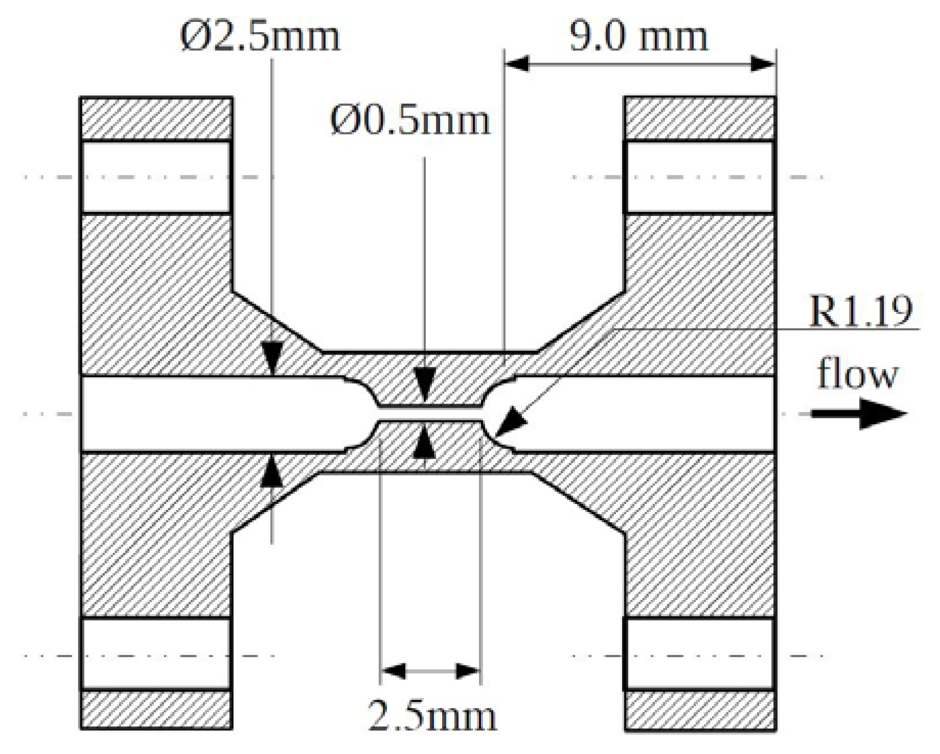
Figure 2.
Experimental arrangement [15]. (a) The raster scan grid where X-ray radiography measurements of void were taken, (b) time-averaged X-ray radiography measurement of the void at CN = 11.2, (c) time-integrated X-ray images of nozzle inlet at CN = 11.2. (Reproduced with permission).
Figure 2.
Experimental arrangement [15]. (a) The raster scan grid where X-ray radiography measurements of void were taken, (b) time-averaged X-ray radiography measurement of the void at CN = 11.2, (c) time-integrated X-ray images of nozzle inlet at CN = 11.2. (Reproduced with permission).
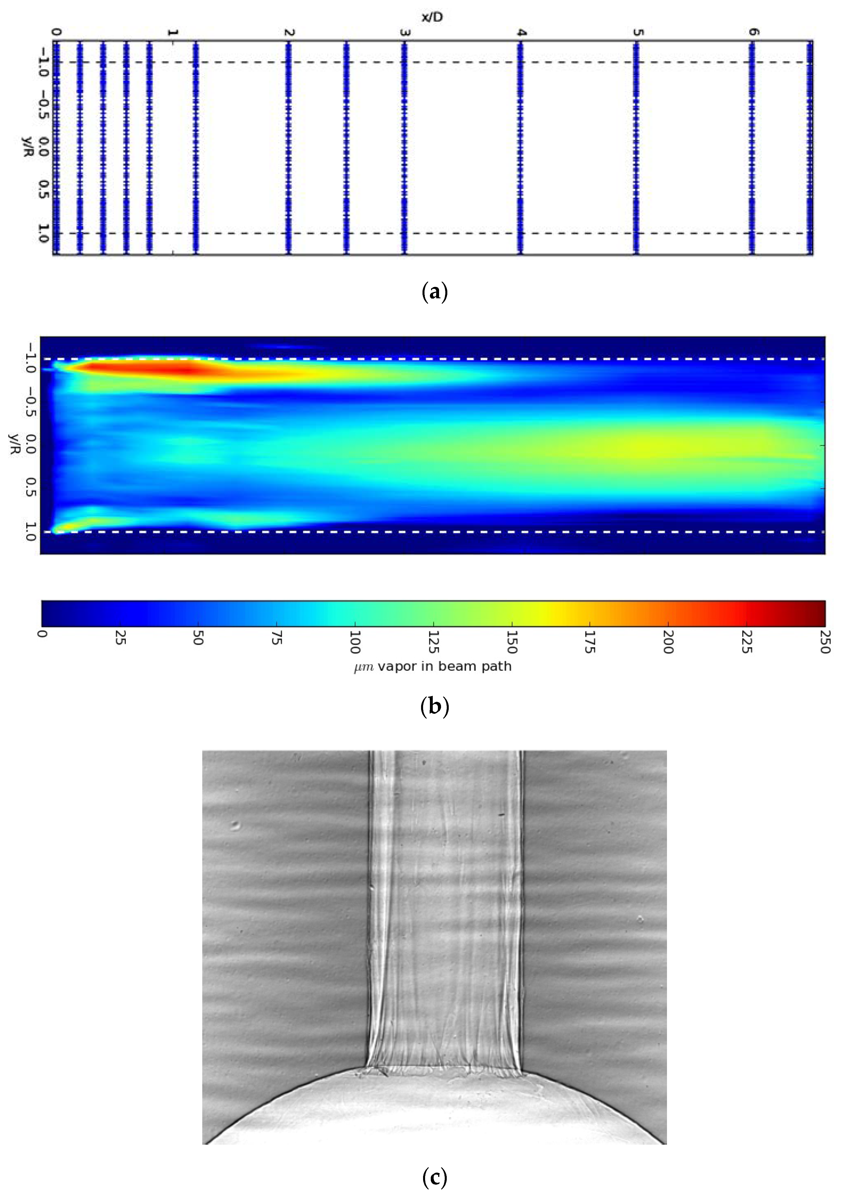
Figure 3.
2D flow axis-symmetric flow domain for the present case: The numbers represent boundaries of flow domains, (1) inlet, (2) outlet, (3) wall, (4) axis.
Figure 3.
2D flow axis-symmetric flow domain for the present case: The numbers represent boundaries of flow domains, (1) inlet, (2) outlet, (3) wall, (4) axis.
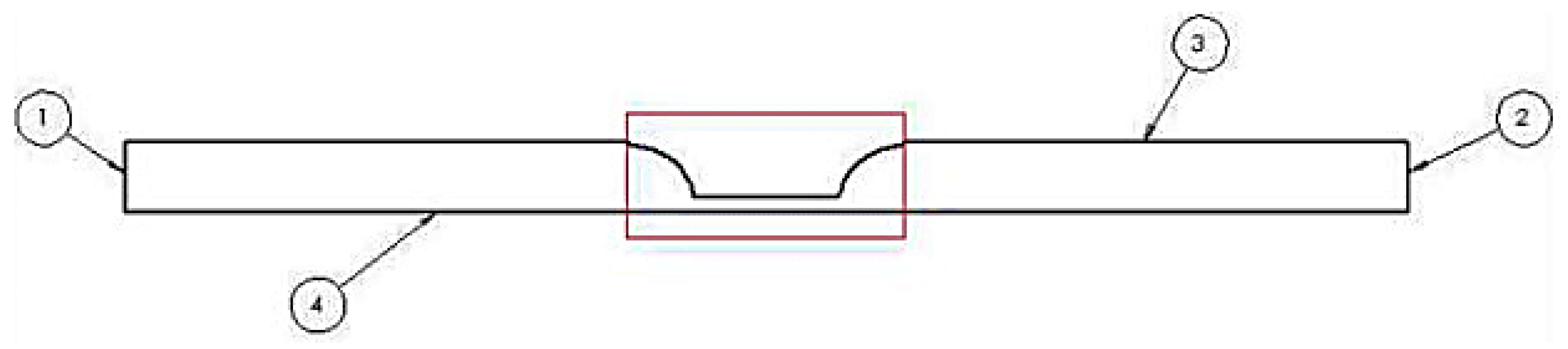
Figure 4.
2D axis-symmetrical unstructured mesh with quad type elements of the nozzle flow domain. The mesh is refined in the circular section near the entrance and the exit of the orifice and in the orifice region.
Figure 4.
2D axis-symmetrical unstructured mesh with quad type elements of the nozzle flow domain. The mesh is refined in the circular section near the entrance and the exit of the orifice and in the orifice region.

Figure 5.
Grid sensitivity study: (a) vapor volume fraction across the nozzle at different axial positions along with the nozzle, (b) axial velocity distribution at x/L = 0.0167.
Figure 5.
Grid sensitivity study: (a) vapor volume fraction across the nozzle at different axial positions along with the nozzle, (b) axial velocity distribution at x/L = 0.0167.
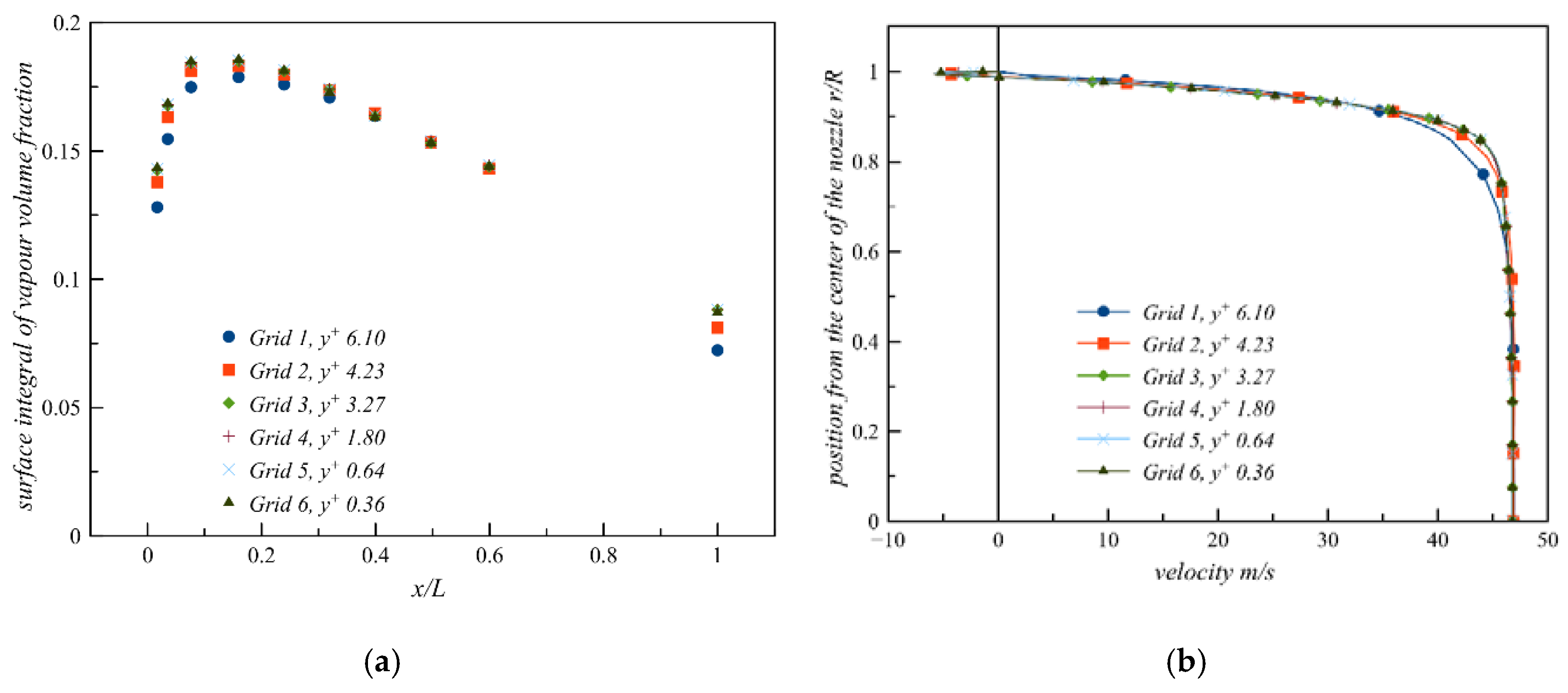
Figure 6.
Comparison of predicted total vapor volume fraction, obtained from four turbulence models, with experimentally measured total vapor volume fraction across the nozzle at different axial positions along the nozzle. Error bars in the experimental data show uncertainty of around 2% [15].
Figure 6.
Comparison of predicted total vapor volume fraction, obtained from four turbulence models, with experimentally measured total vapor volume fraction across the nozzle at different axial positions along the nozzle. Error bars in the experimental data show uncertainty of around 2% [15].
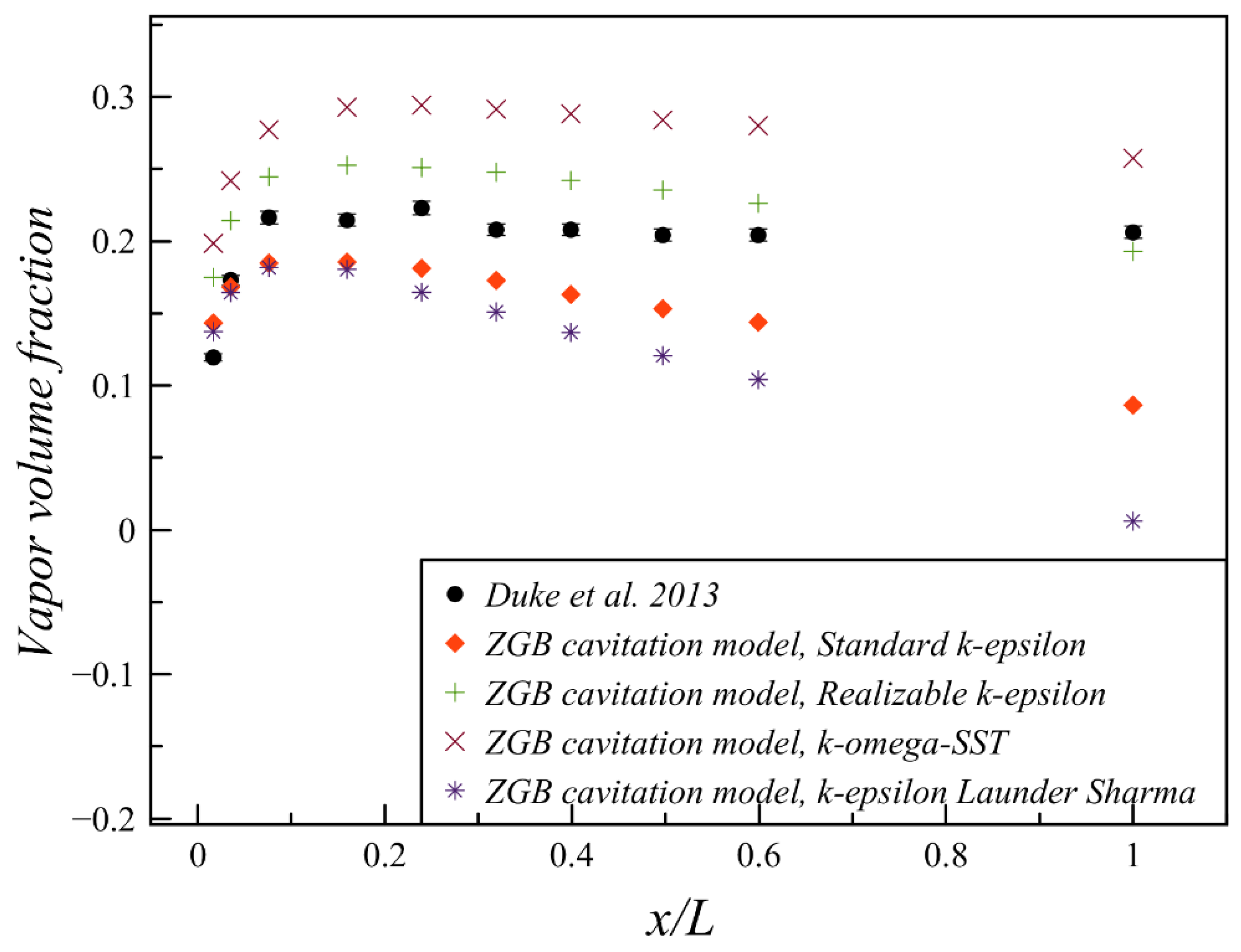
Figure 7.
Qualitative comparison of vapor volume fraction between the experimental and CFD predicted results. (a) X-ray radiography measurement at CN = 11.2 [15], (b) standard k-epsilon, (c) realizable k-epsilon.
Figure 7.
Qualitative comparison of vapor volume fraction between the experimental and CFD predicted results. (a) X-ray radiography measurement at CN = 11.2 [15], (b) standard k-epsilon, (c) realizable k-epsilon.
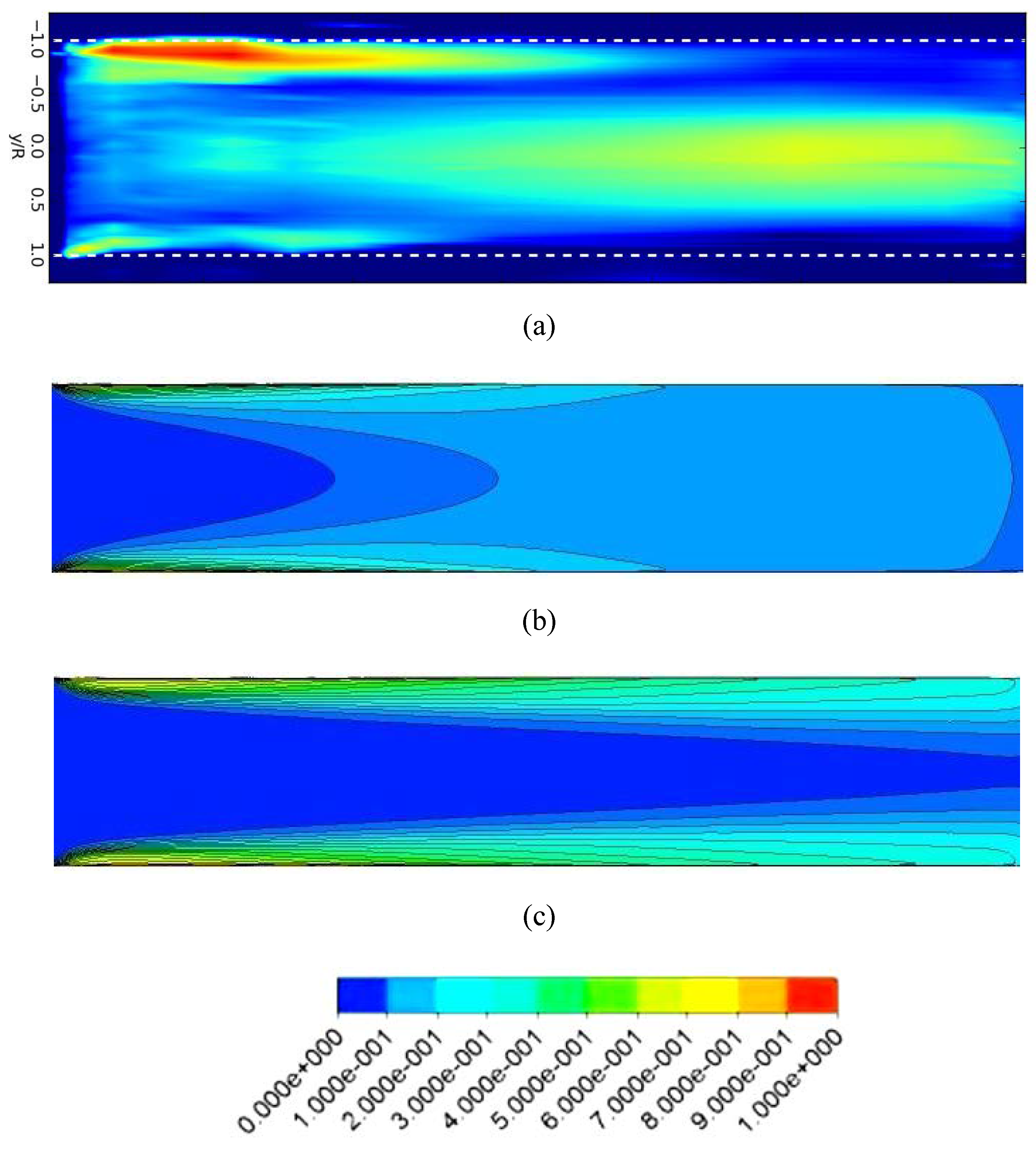
Figure 8.
Comparison of predicted total vapor volume fraction using two cavitation models with experimentally measured total vapor volume fraction across the nozzle at different axial positions along the nozzle. Error bars in the experimental data show uncertainty of around 2% [15].
Figure 8.
Comparison of predicted total vapor volume fraction using two cavitation models with experimentally measured total vapor volume fraction across the nozzle at different axial positions along the nozzle. Error bars in the experimental data show uncertainty of around 2% [15].

Figure 9.
Qualitative comparison between the experimental and CFD predicted results; (a) X-ray radiography measurement [15] (reproduced with permission), (b) Schnerr and Sauer (SS) model, and (c) Zwart-Gerber-Belamri (ZGB) model.
Figure 9.
Qualitative comparison between the experimental and CFD predicted results; (a) X-ray radiography measurement [15] (reproduced with permission), (b) Schnerr and Sauer (SS) model, and (c) Zwart-Gerber-Belamri (ZGB) model.
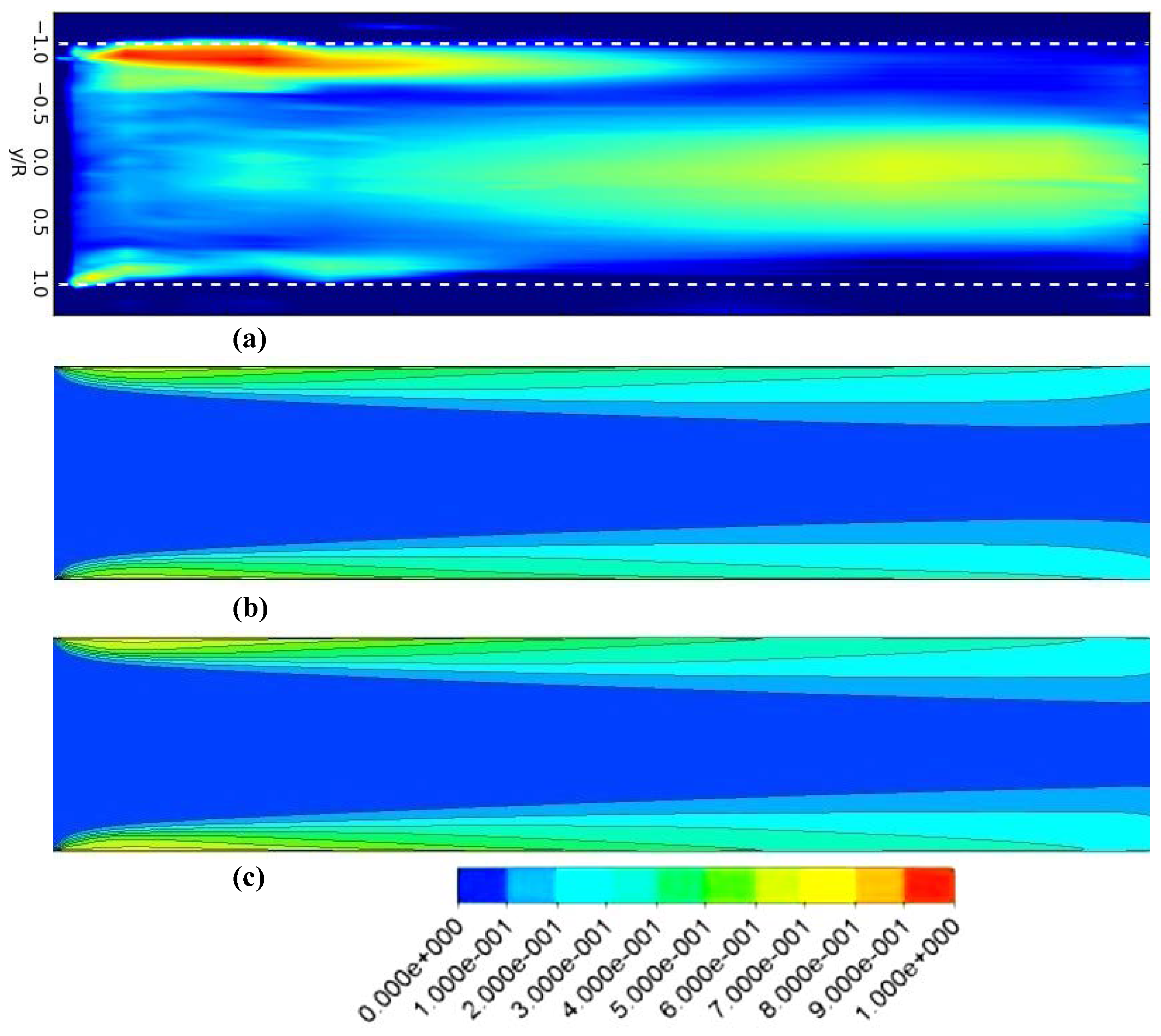
Figure 10.
Visual comparison of vapor volume fraction predicted using two cavitation models; (a) SS model, (b) ZGB model.
Figure 10.
Visual comparison of vapor volume fraction predicted using two cavitation models; (a) SS model, (b) ZGB model.
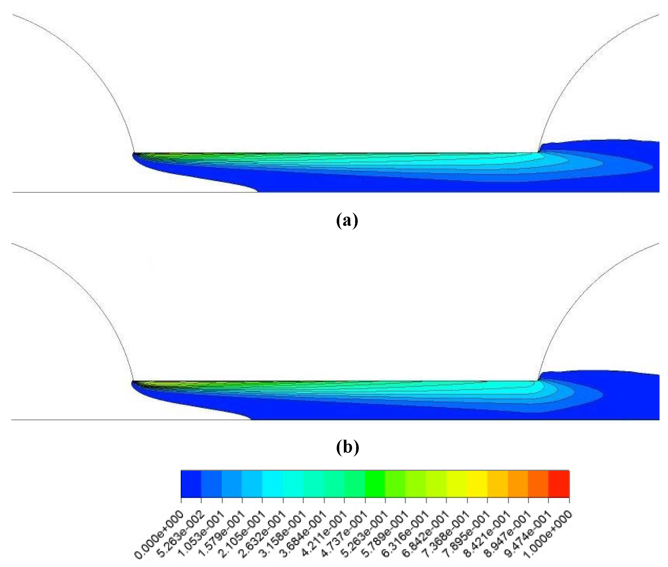
Figure 11.
Comparison of the evaporation and condensation rates of SS and ZGB models; (a) evaporation, (b) condensation.
Figure 11.
Comparison of the evaporation and condensation rates of SS and ZGB models; (a) evaporation, (b) condensation.
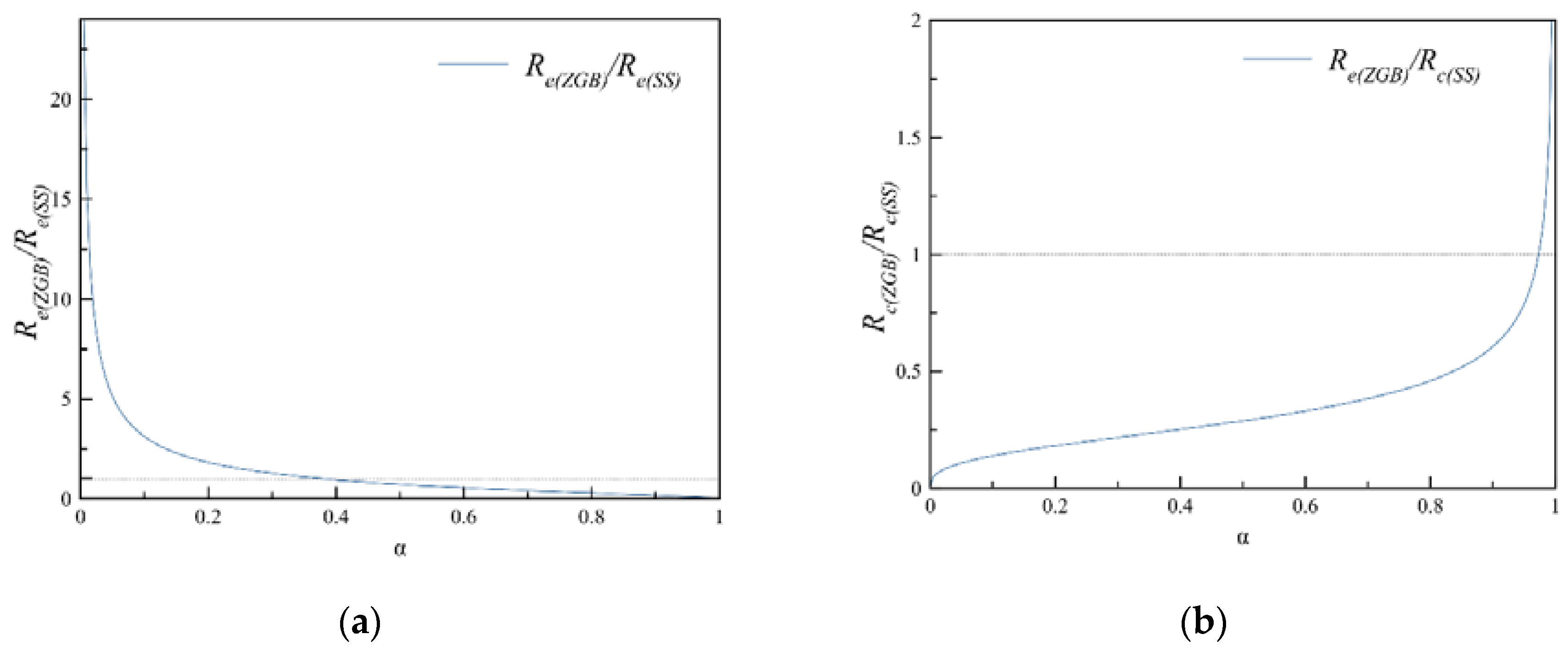
Figure 12.
Influence of model constants on total vapor volume fraction at different axial positions along the nozzle.
Figure 12.
Influence of model constants on total vapor volume fraction at different axial positions along the nozzle.
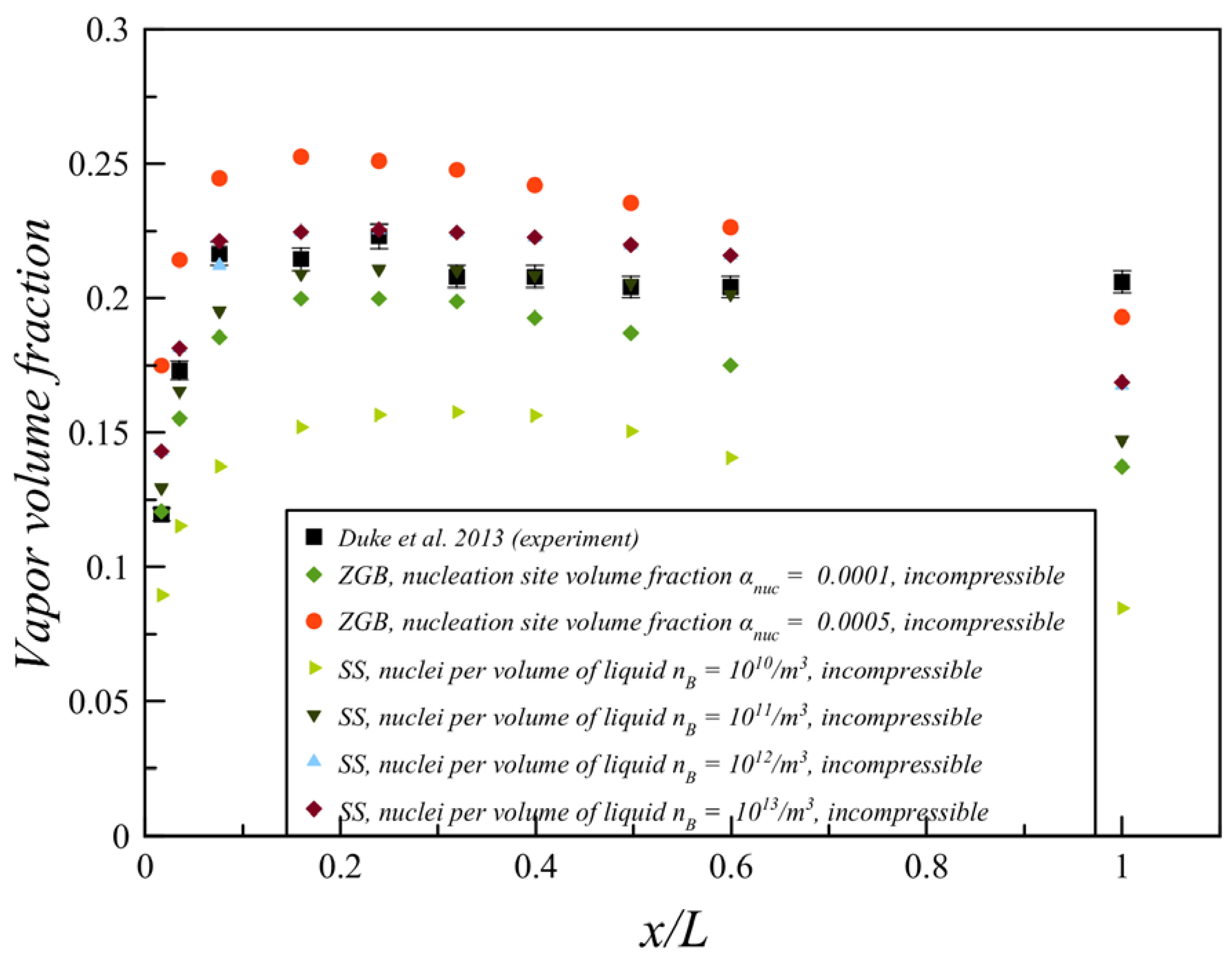
Figure 13.
Comparison between the experimental and CFD predicted results to check the influences of vapor compressibility. (a) X-ray radiography measurement at CN = 11.2 [15], (b) SS model, incompressible, , (c) SS model, compressible, , (d) ZGB model, incompressible, = 0.0001, (e) ZGB model, compressible, = 0.0001.
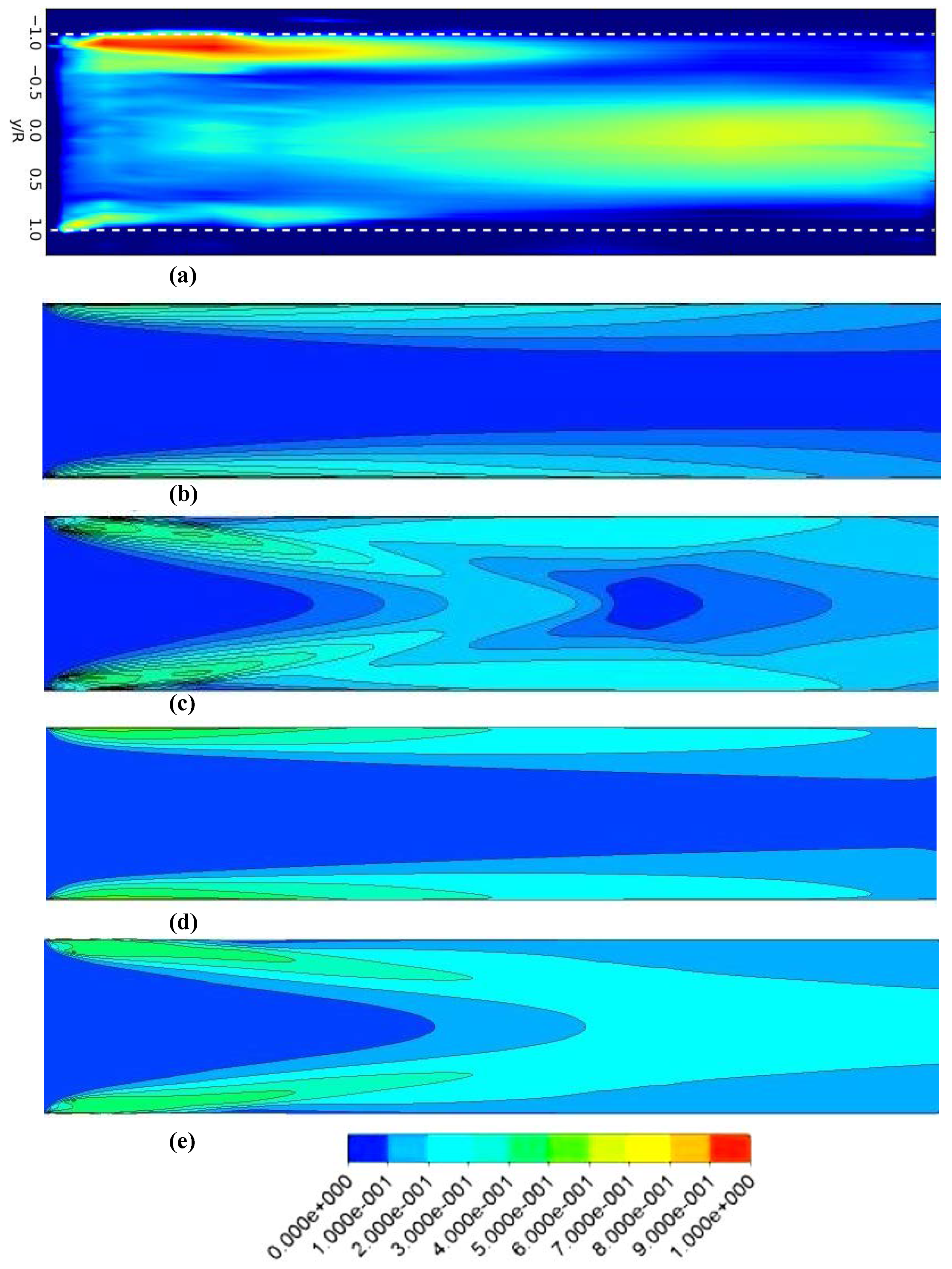
Figure 14.
Influence of compressibility on total vapor volume fraction at different axial positions along the nozzle.
Figure 14.
Influence of compressibility on total vapor volume fraction at different axial positions along the nozzle.
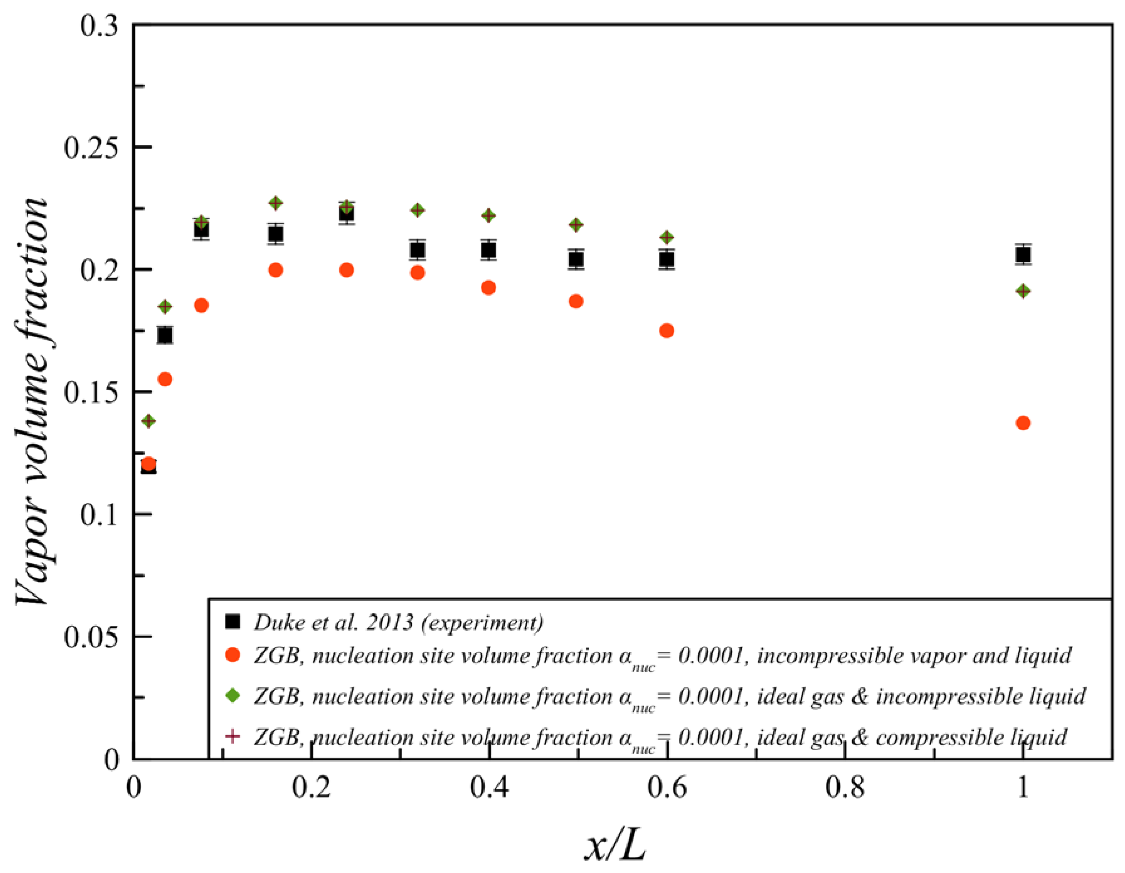
Figure 15.
Predicted distribution of vapor volume fraction and absolute pressure across the nozzle; (a) vapor volume fraction, (b) pressure (Pa).
Figure 15.
Predicted distribution of vapor volume fraction and absolute pressure across the nozzle; (a) vapor volume fraction, (b) pressure (Pa).
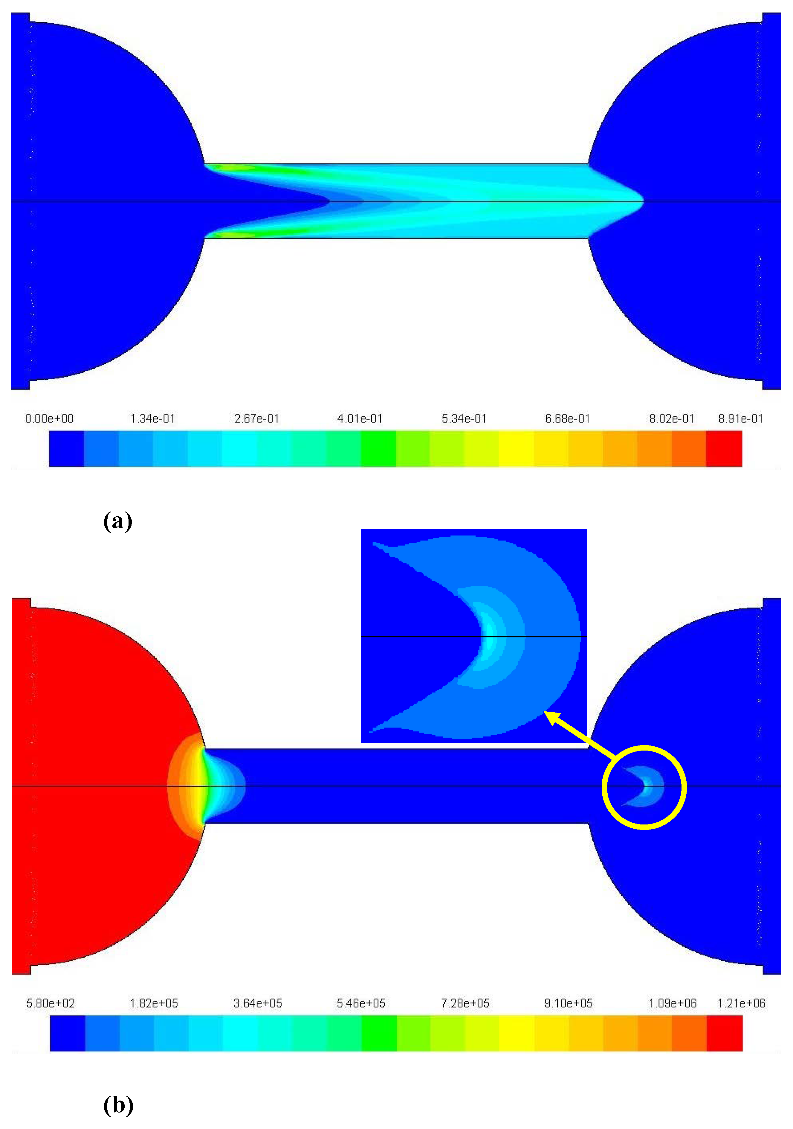
Figure 16.
Predicted pressure and velocity profiles on the nozzle axis. (a) Pressure profile, (b) velocity profile.
Figure 16.
Predicted pressure and velocity profiles on the nozzle axis. (a) Pressure profile, (b) velocity profile.
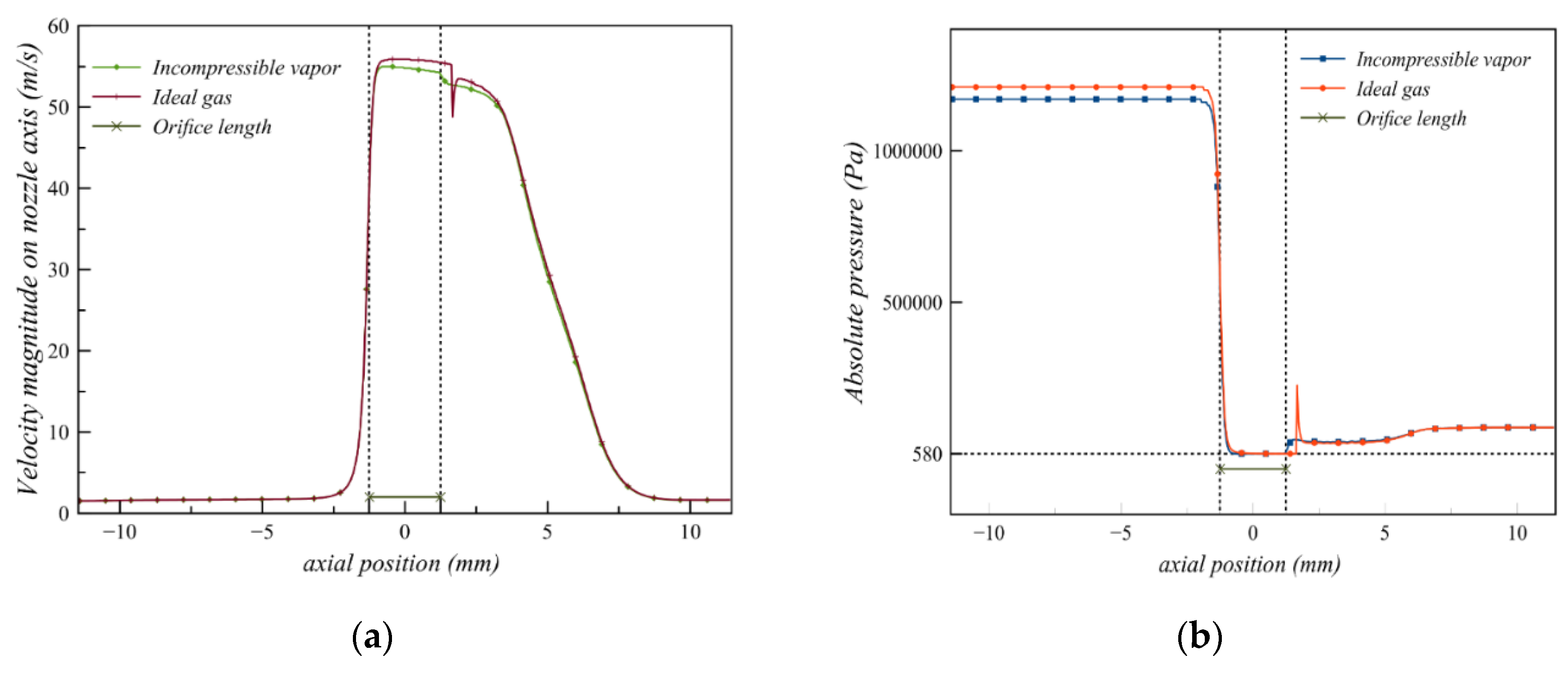
Figure 17.
Comparison of the speed of sound in vapor , liquid , and the mixture phase with the velocity at the nozzle axis.
Figure 17.
Comparison of the speed of sound in vapor , liquid , and the mixture phase with the velocity at the nozzle axis.

Table 1.
Operating conditions of the experiment.
| Fuel Flow Rate [L/hr] | Reynolds Number, Re | Cavitation Number, CN | T [°C] | ||
|---|---|---|---|---|---|
| 1060 ± 60 | 87 ± 2 | 26.8 ± 0.24 | 15,800 | 11.2 | 25 |
Table 2.
Reference values used in Tait equation.
| 101,325 | 777.97 |
© 2020 by the authors. Licensee MDPI, Basel, Switzerland. This article is an open access article distributed under the terms and conditions of the Creative Commons Attribution (CC BY) license (http://creativecommons.org/licenses/by/4.0/).
Share and Cite
MDPI and ACS Style
Kumar, A.; Ghobadian, A.; Nouri, J.M. Assessment of Cavitation Models for Compressible Flows Inside a Nozzle. Fluids 2020, 5, 134. https://doi.org/10.3390/fluids5030134
AMA Style
Kumar A, Ghobadian A, Nouri JM. Assessment of Cavitation Models for Compressible Flows Inside a Nozzle. Fluids. 2020; 5(3):134. https://doi.org/10.3390/fluids5030134
Chicago/Turabian StyleKumar, Aishvarya, Ali Ghobadian, and Jamshid M. Nouri. 2020. "Assessment of Cavitation Models for Compressible Flows Inside a Nozzle" Fluids 5, no. 3: 134. https://doi.org/10.3390/fluids5030134