NARMAX Identification Based Closed-Loop Control of Flow Separation over NACA 0015 Airfoil


1
MAE Department, Clarkson University, Potsdam, NY 13699, USA
2
Department of Mechanical Engineering, Rowan University, Glassboro, NJ 08028, USA
*
Authors to whom correspondence should be addressed.
Fluids 2020, 5(3), 100; https://doi.org/10.3390/fluids5030100
Submission received: 1 April 2020
/
Revised: 2 June 2020
/
Accepted: 22 June 2020
/
Published: 29 June 2020
(This article belongs to the Special Issue Recent Advances in Fluid Mechanics: Feature Papers)
Abstract
:A closed-loop control algorithm for the reduction of turbulent flow separation over NACA 0015 airfoil equipped with leading-edge synthetic jet actuators (SJAs) is presented. A system identification approach based on Nonlinear Auto-Regressive Moving Average with eXogenous inputs (NARMAX) technique was used to predict nonlinear dynamics of the fluid flow and for the design of the controller system. Numerical simulations based on URANS equations are performed at Reynolds number of 106 for various airfoil incidences with and without closed-loop control. The NARMAX model for flow over an airfoil is based on the static pressure data, and the synthetic jet actuator is developed using an incompressible flow model. The corresponding NARMAX identification model developed for the pressure data is nonlinear; therefore, the describing function technique is used to linearize the system within its frequency range. Low-pass filtering is used to obtain quasi-linear state values, which assist in the application of linear control techniques. The reference signal signifies the condition of a fully re-attached flow, and it is determined based on the linearization of the original signal during open-loop control. The controller design follows the standard proportional-integral (PI) technique for the single-input single-output system. The resulting closed-loop response tracks the reference value and leads to significant improvements in the transient response over the open-loop system. The NARMAX controller enhances the lift coefficient from 0.787 for the uncontrolled case to 1.315 for the controlled case with an increase of 67.1%.

1. Introduction
Efficient and safe design of aircraft, missiles, propellers, turbines, compressors, automobiles, ships, trains, and civil engineering structures depend to a far extent on an understanding of the nature of flow around bodies (Gad-el-Hak [1]). Aircraft wings are typically evaluated according to their aerodynamic performance, mainly measured in terms of lift to drag ratio. At high angles of attack, airfoils suffer from flow separations and significant loss of aerodynamic performance.
Separation is defined as the detachment of the fluid flow from a solid surface. Whether caused by an adverse pressure gradient, a geometric disruption, or by any other means, separation is generally associated with significant thickening of a rotational flow region adjacent to the airfoil surface and by an increase in the velocity component normal to the surface (Simpson [2]). Flow separation always causes adverse effects on airfoil performance, such as reduced lift, increased drag, noise emissions, and airfoil buffeting. This decrease in airfoil performance, which could lead to the stall regime, can be avoided or delayed with the use of flow control techniques (Benard et al. [3]).
When the flow separation flow cannot be avoided, it is important to understand the effects of separation on a specific design (Mable et al. [4]). In particular, aerospace researchers are continually searching for efficient methods to improve the aerodynamic efficiency of flight vehicles. The main goals of flow control are to improve performance characteristics by avoiding a stall, reducing drag, enhancing lift, and abating noise. The specific objectives of flow control are usually achieved through one of the following: (1) delay or eliminate flow separation; (2) delay boundary layer transition; or (3) reduce skin friction drag (Huebsch et al. [5]).
From an aerodynamic perspective, proper flow control schemes have the ability to manipulate the flow and improve the performance features by reducing skin friction and form drag, increasing lift, improving flight controllability and maneuverability, and providing significant savings in overall fuel consumption. For example, maintaining laminar flow over the entire wing surface can reduce total aircraft drag by as much as 15% (Schrauf [6]). In the commercial aircraft industry, overall drag reduction of just 1% can lead to millions of dollars of saving in annual fuel costs (Huebsch et al. [5]).
The capability to actively or passively control the flow around an object to achieve an enhanced performance is of great value (Joslin and Miller [7]). Various passive and active separation control approaches have been tested with different degrees of success. Passive control techniques encompass approaches that lead to geometric modifications to change the flow features, while active control techniques utilize actuators to modify the flow and therefore require external energy (Cattafesta et al. [8]). Passive flow control for aircraft wings includes leading-edge slats, trailing edge slotted flaps, or a combination of the two. Another passive flow control device is the vortex generators, which are relatively small rigid fixtures that are placed on the top surface of an airfoil. However, vortex generators increase drag, and due to their nature of being fixed on the surface of the airfoil, they decrease the efficiency of flight when they are not needed. Passive actuation also includes such devices as riblets, spoilers, strakes, and steady suction or blowing.
Passive flow control methods have been a field of considerable interest since long ago and found abundantly in the aerospace industry. The main merit of passive control over an active control is its simplicity to implement, tendency to be lighter, less expensive to design and manufacture, and easier to maintain. Hence passive control techniques are more likely to be used in real-world applications (Williams et al. [9]). The passive control methods, however, may only be effective over a restricted range of operating conditions. The system performance may even be deteriorated under certain conditions with the use of passive control. The disadvantages of current designs are that they add mechanical complexity to the wing design, take up the volume when not in use, add weight, and generate vibration and noise. Likewise, since most engineering flows contain complex unsteady motions (instabilities, turbulence), the ability of a passive device to control these unsteady motions is inherently limited. Examples of passive flow control applications can be found in (Bechert et al. [10]; Fisher et al. [11]; Kaplanski et al. [12,13]; Hussainov et al. [14,15]).
Active flow control (AFC) is an enabling technology as fluid dynamics, controllers, actuators, and sensors merge to form advanced control systems capable of modifying flow behavior under challenging aerospace applications (Joslin and Miller [7]). Actuators and sensors become increasingly more powerful, cheaper, and more reliable to be considered for practical applications (Noack et al. [16]). AFC provides numerous advantages over passive methods. When not needed, active control devices may be turned off, and they could also adjust to the changes in the flow conditions (Williams et al. [9]). AFC technology typically used small, localized energy input to alter the flow. Active control can be utilized to control dynamical flow patterns such as turbulence to reduce skin friction drag.
In boundary layers, the turbulence production mechanism is a complex series of dynamical events associated with organized, near-wall streaks and their instabilities. This process results in sudden bursts of low-momentum fluid away from the wall. Bushnell [17] reported that the correct phasing of the control inputs with respect to the organized flow patterns could be the cause for the success of a control algorithm. In this respect, Lumley and Blossey [18] described the applications of active control of turbulent flow by modifying the production of turbulence.
Flow sensors need to be robust and not significantly alter the flow field that is measured. Flow sensors should possess sufficient spatial and temporal resolution to accurately capture the relevant flow physics to be controlled (Cattafesta et al. [19]). For practical reasons, most flow sensors for AFC are flush-mounted on a solid surface. Typically, at the solid surface, the wall pressure and/or skin friction can be measured. For cases in which the wall pressure is important, there are many devices for measuring pressure changes, which are essentially small microphones. Many flow sensors fall under the categories of classical, optical, and Micro Electro Mechanical Systems (MEMS). Some examples of sensors for measuring wall shear stress include floating element sensors, hot films, and shear stress crystals.
There are various ways to classify flow control actuators, including type (e.g., fluidic, thermal, acoustic, and plasma), transduction scheme (piezoelectric, electromagnetic, electrodynamic, and electrostatic), output form (constant blowing, constant suction, periodic excitation, and synthetic jets) and structural design (shape memory alloys, MEMS, Nano-elements). The input to an actuator is an electrical quantity that produces an output flow perturbation. The most critical design parameters for active flow actuators are the control authority (or stroke) and the bandwidth. Unfortunately, these two parameters conflict with one another. A rise in stroke usually led to decreased bandwidth (Mathew et al. [20]). The design objective usually requires that the actuator generates sufficient stroke over a range of frequencies to generate the appropriate control effects. Low power consumption, rapid response, reliability, and low cost are appropriate characteristics of actuators.
Active control may be categorized as predetermined (open loop) or reactive (closed-loop). Predetermined control includes the application of steady or unsteady energy input regardless of the particular state of the flow with no need for sensors. Most cases of AFC require parameter adjustments for flow conditions and occasionally real-time response using flow sensors. Closed-loop flow control offers a promising alternative to passive (no power) and active open-loop (no sensing) flow control approaches. It relies on small-scale powered actuators, forcing the flow dynamically in response to a sensor signal transformed by control law. The key advantage of feedback control lies in the ability of the controller to adapt to changes in exogenous parameters and to modify the dynamics of the flow system.
Examples of steady jet control techniques can be found in the works of Wong and Kontis [21], and Eldredge and Bons [22]. For the case of unsteady jet actuation, readers are referred to Shan et al. [23], Seifert et al. [24], and Amitay and Glezer [25]. The steady or quasi-steady-state of increasing lift enhancement and reducing drag at relatively low chord Reynolds number (typically <0.5 million) were considered in these studies. Using periodic excitation that making use of natural flow instability has the ability to overcome the efficiency barrier. Seifert et al. [26] reported that separation control excitation, at frequencies somewhat higher than the vortex shedding frequencies, leads to 90–99% saving of the momentum needed to achieve results in performance with steady blowing. Closed-loop separation control has not yet received significant attention in experimental studies. In addition, the characteristics of hardware needed (sensors, actuators, and real-time control systems) impose significant limits on the complexity of the closed-loop control system (Billings and Leontaritis [27]).
Recently a variety of closed-loop separation control techniques have been developed for a wide range of applications and geometries.
Nishizawa et al. [28] successfully conducted experiments on the NACA 0015 airfoil wing model to control leading-edge separation using a closed-loop system composed of a flow-direction discriminator, a simple control algorithm, and disturbance actuators. Later in 2005, Nishizawa et al. [29], designed PID closed-loop controllers for both NACA 0015 and MEL001 airfoils flow separation control using Micro Jet Vortex Generators (MJVG). Applications of MJVG on a MEL001 airfoil at Re = 104 to 105 gave an appreciable increase in the lift coefficient (Abe et al. [30]). An alternative suction/blowing jet (ASBJ) was developed, and in a preliminary experiment, its drag reduction effect was observed (Segawa et al. [31]).
Tian et al. [32] implemented an adaptive closed-loop to control flow over NACA 0025 airfoil utilizing zero-net-mass flux (ZNMF) actuators. In another work, Tian et al. [33] also implemented an adaptive disturbance rejection control algorithm with system identification using synthetic jet actuators and two dynamic pressure sensors. The objective was to minimize the unsteady pressure fluctuations over the airfoil, which results in up to ~5 dB of power reduction and ~5× improvements in the lift/drag ratio. Song et al. [34] used the same set-up with MIMO generalized predictive control algorithm. The results showed 7× improvements in the lift/drag ratio with less computational cost compared to Tian et al. [32].
Pinier et al. [35] used a proportional controller based on a low order model to control separation on NACA 4412 airfoil using piezoelectric synthetic jet actuators. The unsteady pressure measurements were used to estimate the proper orthogonal decomposition (POD) coefficients for the model. Later on, Ausseur et al. [36] used the same set-up with different techniques of reduced-order modeling based on a combined technique of Proper Orthogonal Decomposition and Linear Stochastic Estimations (POD/LSE) and taking the estimated temporal coefficient of first POD mode as control candidate.
Becker et al. [37] conducted an experimental investigation on NACA 4412 airfoil using Single-Input Single-Output SISO extremum seeking control using pulsed jet actuator over a two elements high lift configuration. They extended it to the SISO slope seeking control to avoid saturation of the control input. Finally, for more realistic 3-D flight configurations, span-wise MIMO slope seeking control was used. The pressure gradient on the flap was used as the criterion for reattachment. For non-model based adaptive control, slope seeking approach was developed as a new concept which involves driving the output of a plant to a value corresponding to a guided slope of its reference-to-output chart. The extremum seeking scheme is a special case of slope seeking in which the guided slope is zero. Examples of closed-loop control algorithms for flow separation control can be found in the works done by Allan et al. [38], Becker et al. [39], Henning and King [40], Becker and King [41], Duvigneau and Visonneau [42], Bourgois [43], Cattafesta et al. [44], Cho et al. [45], Taira et al. [46], Benard et al. [47], Luchtenburg et al. [48], Colonius et al. [49].
Most experiments on flow control have used a backward-facing step or different NACA airfoils. A variety of actuators has been used, while sensors were mostly pressure transducers. Also, a large variety of controllers were used. Most of the studies were at relatively low Reynolds ( to 5 × ) except that by Allan et al. [38], where the chord Reynolds number was 16 million.
Over the last few years, much attention from the fluid dynamic research community has been given to the development of synthetic jet actuators (SJA) or “zero mass flux” devices. Also, SJAs are preferable as they characterized by a small, low- energy, typically high-frequency actuators, in which the operation is based on the concentrated input of energy at high receptivity regions of the flow field. A variety of promising flow control applications based on synthetic jet actuators have been presented. Numerous investigations on synthetic jet have shown that flow separation can be diminished or even eliminated entirely (Tuck and Soria [50] Amitay and Glezer [51]; He et al. [52]; Amitay et al. [53]; Crook et al. [54]; Seifert and Pack [55]; Amitay et al. [56]; Smith et al. [57]; and Seifert et al. [26]). Synthetic jets have also been used for separation control in inlet ducts (Amitay et al. [58]). SJAs were also utilized on an unmanned aerial vehicle (Parekh et al. [59]), flight control on scaled models (Ciuryla et al. [60]), as well as jet vectoring (Smith and Glezer [61]). Maldonado et al. [62] used SJA for control of wind turbines’ vibrations. Chatlynne et al. [63] and Amitay et al. [64]) used the synthetic jets for flow control over a 2-D airfoil at low angles of attack, where the flow is fully attached. Application to 3-D configurations was reported by Farnsworth et al. [65].
Timor et al. [66] reported that in some cases using synthetic jets, considerable control forces were exerted by cropping the trailing edge of an airfoil. These suggest the potential for replacing the classical control surfaces (flaps, aileron, rudder) with AFC or at least improve their performance in terms of control authority as well as frequency response. Darabi and Wygnanski [67,68] described their investigations dealing with the transient flow attachment and separation in response to a synthetic jet actuator.
And Amitay and Glezer [25,69]. More recently, Mathis et al. [70] performed a similar study using a steady jet to provoke separation for enhancement of mixing. In the current research, we utilize SJA as an actuator and investigate the performance of the control system to modify the lift and drag of 2-D airfoils.
The ability to simulate aerodynamic flows utilizing Computational Fluid Dynamics (CFD) has advanced rapidly during the last several decades and has fundamentally changed the aerospace design process. Recently, the increasingly crucial role of the CFD in the fields of analysis, design, certification, and support of aerospace products has been described by many researchers. The utilization of CFD codes has become standard engineering practice to examine flow physics around geometrically complicated shapes (Jones and Clarke [71]). Advanced simulation capabilities of CFD codes do not only enable reductions in ground-based and in-flight testing requirements, but also provide added physical insight, enabling superior designs at reduced cost and risk, and open new frontiers in aerospace performance (Slotnick et al. [72]). CFD codes provide numerical approaches for solving the governing equations of the fluid motion, which are mainly the Navier-Stokes (N–S) or the Reynolds averaged Navier-Stokes (RANS) equations.
An additional element stimulating new developments in AFC occurred in the 1990s when CFD was used as a tool to explore new concepts in AFC. The CFD, coupled with the control theory, proved to be a powerful combination leading to improved understanding of the flow physics. Not only were numerical simulations useful in providing details about the flow, but they were more amenable than experiments to the integration with modern control theory (Choi et al. [73], Kim [74]). Application-oriented simulations for flow control was found to be useful for determining locations for high receptivity to actuator and sensor placement, and for obtaining scaling information needed for full-scale application.
Given the extensive computing requirements, it has been known that real-time solutions of the Reynolds averaged Navier-Stokes (RANS) equations for control applications would not be feasible in practical situations. The development of reduced-order models has enabled closed-loop flow control to be implemented for many cases. Some non-model based control algorithms have attracted attention as they alleviate the difficulties of modeling separated flow while achieving the control goals. Methods used in the works reported by Banaszuk et al. [75], Becker et al. [40], Becker et al. [37], Tian et al. [31], Tian et al. [32] and Benard et al. [47] are capable of “training” the excitation signals to be most effective in terms of objective functions (i.e., pressure recovery, and lift-to-drag ratio). The main drawback of these methods is that they work on the time-averaged objective functions as they operate on a time scale that is much larger than that of the flow dynamics. For non-model based flow control, the well-known system identification (ID) schemes are utilized to model the system dynamics, including the actuator and unsteady surface pressure sensors. The system to be identified includes the dynamics of the actuators, flow structures excited by SJA, and dynamics of the sensors. Information contained in this system information is then utilized to predict the subsequent evolution of the pressure fluctuations around the airfoil. An attractive scheme for discrete systems employed in control applications is the NARMAX model, where the system output can be forecasted utilizing the past input and output lags of the system. Chen and Billings [76] proposed the NARMAX approach to represent the discrete nonlinear systems.
The NARMAX is a nonlinear autoregressive moving average model that can represent a broad class of nonlinear systems. The approach provides the ability to construct the model sequentially by determining the most critical term and then determining and adding the next important term, and so on. Therefore, the model is constructed step by step until the desired accuracy is achieved (Billings [77]). The NARMAX power-form polynomial identification of nonlinear systems offers many advantages over other nonlinear difference equation structures (Liu [78]). The model has an explicit recursion in the present output y(t), and it is suitable for modeling both the stochastic and deterministic systems and is capable of describing a wide variety of nonlinear systems (Leontaritis and Billings [79]). The resulting model is linear, which enables the application of well-established parameter estimation techniques developed for linear system identification. Although NARMAX is capable of describing a wide variety of nonlinear systems, it has been mainly used for control problems. The NARMAX representation provides an alternative to block-structured models (Liu [78]). Several successful applications of polynomial NARMAX models were reported in the literature demonstrating its application in system identification (Thomson et al. [80]; Swain et al. [81,82]; and Kukreja and Brenner [83]).
In the current study, the NARMAX approach is utilized to construct a feedback control subroutine for flow separation on NACA 0015 airfoil with leading-edge SJA mounted at 10% chord length. The purpose is to obstruct flow separation or stall by maintaining the flow attached to the surface of the airfoil. Here, the flow model is built by using the synthetic jet velocity as input and pressure as an output. Hence, it is suitable to construct a SISO system identification dynamic model directly via parameter estimation of input-output data relationships.
With the NARMAX method, the Airfoil-SJA system is modeled in terms of the difference equations relating the current output to combinations of inputs and past outputs.
The flow around the NACA 0015 airfoil was first modeled using the ANSYS-FLUENT code in a series of studies. The airfoil geometry was constructed, and the computational domain was identified and meshed. The boundary conditions were set, and the Reynolds Averaged Navier Stokes (RANS) equations were solved. The mesh independence studies were performed, and then the RANS simulations were conducted, and the flow patterns around the airfoil at various incidence angles were evaluated. Fluent simulation results were validated using experimental data obtained from wind tunnel testing of flow over a model of 30 cm chord length and 40 cm span at Re = . Simulation results provided core information for the baseline case (no control) at AoA = 16° that used for control purposes. In addition, the flows around the airfoil with synthetic jet actuators (SJAs) were considered, and the RANS simulations were performed for the control-on cases when the synthetic jet actuator was active. Information obtained from open-loop control was used to develop a closed-loop control algorithm.
For implementing linear control, a NARMAX model for flow over airfoil based on the static pressure data and the synthetic jet actuator was developed using the data from the incompressible flow simulations results for cases with and without SJAs. The describing function technique was used for linearization of the identified pressure signal within its frequency range, and then a low pass filtering was used to provide quasi-linear state values (linear in plant/nonlinear in instrumentation), which was used in the application of the quasi-linear control techniques. Quasi-linear control techniques are similar to the linear control techniques and used in cases where the plant can be viewed as linear, but the instrumentation, i.e., the actuators and sensors, cannot (Ching et al. [84]). The desired pressure signal that signifies the condition of fully re-attached flow over the airfoil surface was selected based on the linearized original pressure signal reported by the sensor during open-loop control.
The closed-loop control algorithm was designed and inspected in the MATLAB Simulink environment. The controller design followed the standard proportional-integral (PI) approach for single-input single-output systems. The results showed that the closed-loop response tracks the reference value reasonably well and leads to significant improvements in the transient response over the open-loop system. The NARMAX based controller enhanced the lift coefficient of the NACA 0015 airfoil at AoA = 16° from 0.787 for the uncontrolled case to 1.315 for the controlled case with an increase of 67.1%.
2. Numerical Simulation of Flow over the NACA 0015 Airfoil
Flow over airfoils at high angles of attack and its control is quite complicated due to the flow separation that leads to vortex shedding from both the leading and trailing edges of the airfoil (Wu et al. [85]). Secondary and tertiary separations from the middle part of the airfoil upper surface may also be induced, which makes the airflow field inherently unsteady. Therefore, understanding the mechanisms of post-stall lift enhancement by unsteady controls, which requires careful numerical simulations and detailed experimental studies, has attracted considerable attention.
Motivated by these needs, in this study, a series of two-dimensional URANS simulations of airflow around NACA 0015 airfoil are performed to study the separation control capabilities of synthetic jet actuators. The effect of the actuators on the lift characteristics of the airfoil is investigated. A close examination of the controlled and uncontrolled flow fields reveals the features of the airflow that are difficult to observe via experimentation. The ANSYS-FLUENT software is used for the flow simulations, while the MATLAB package is used for the analysis and design of the controller.
A MATLAB script is constructed to simulate the geometry of NACA 0015 airfoil (Abbott, and Von Doenhoff [86]). The dataset for the NACA 0015 airfoil geometry (with 602 points around the airfoil contour) together with the computational domain that was constructed surrounding the airfoil is preprocessed by using the design modeler platform. Finally, the mesh generating tool complementing the software package was used to generate the mesh around the NACA 0015 airfoil.
A structured 2-D C-grid topology of a semi-elliptical shape is used in the present work. In order to attain a fully developed flow, the computational domain with semi-major diameter 43.5 c and semi-minor diameter 10 c, where c is the chord length, is selected and utilized. The semi-elliptical shape of the computational domain provides major advantages over the conventional rectangular and semicircle upstream and rectangular downstream configurations. Dolle [87] recommended this mesh configuration as it leads a considerable reduction in the needed number of cells in the mesh in the far-field, thus allowing for the majority of the cells in the mesh to be concentrated around the airfoil.
The main benefit of this class of mesh is its easy adaptation. The same mesh can also be utilized for different angles of attack by only shifting the tail part of the mesh at the airfoil trailing edge in accordance with the specific angle of attack. To achieve this objective, it was made sure that the straight segment of the elliptic domain has sufficient length to include the incoming flow for all inspected angles of attack (Duvigneau and Visonneau [88]). The distance from the airfoil trailing edge to the downstream pressure far-field boundary is 30 c. The majority of the mesh cells are clustered around the airfoil surface. The domain with these adequately large dimensions was chosen to contain flow disturbances created by the airfoil and to avoid unphysical reflections from the outer boundaries of the mesh. Based on the 4-node quadrilateral elements structure, the grids constructed for this study has about 107,000 cells and 109,000 nodes. Refined quadrilateral cells were placed on top of the boundary layer grid on the upper side and the lower side of the airfoil outline. In addition to this and in order to capture flow features properly in the wake region, Dolle [87] recommended the utilization of a fine grid with quadrilateral cells in these areas rather than other types of cells. The pressure far-field at the fluid domain periphery, velocity-inlet at the SJA location, and wall at the airfoil surface were chosen as boundary conditions during this simulation. Additionally, a velocity boundary condition modeled by a sinusoidal function (in space and time) is developed to fulfill the perturbation effect of periodic jets in the vicinity of the actuator. The schematic of the computational domain and location of the airfoil with boundary conditions is shown in Figure 1.
In this paper, the realizable k-ε turbulence model is used for solving the Unsteady Reynolds Average Navier–Stokes (URANS) equations for the simulation of flow around the NACA 0015 airfoil with and without synthetic actuators. The ANSYS-FLUENT code solves the equations of conservation of mass and balance of momentum together with the transport equations of the realizable k-ε turbulence model. In some cases, the mesh is adapted based on the static pressure gradient, so the solver periodically refines the mesh in the vicinity of regions with substantial pressure variations. A time-dependent pressure-based solver is used in the analysis. Air is treated as an ideal gas with Sutherland Law for viscosity variation. A simple scheme with a Green-Gauss cell-based gradient implicit formulation of pressure velocity coupling is used.
For a free stream velocity of 50 m/s, the flow Reynolds number based on the airfoil cord is Re = 106. Here the free stream ambient temperature is 300 K, the air density is ρ = 1.225 kg/m3, and the air viscosity is kg/ms. For these conditions, the airflow is treated as being incompressible. A segregated, implicit solver is utilized to simulate the flow. The second-order upwind differencing scheme is utilized for spatial discretization. For computing viscous flows, the second-order upwind differencing formulation offers several advantages over a central-differencing scheme (Anderson and Bonhaus [89]). The temporal resolution with a fixed time-stepping method with a time step size (∆t) is set at 0.000125 (s) was utilized. To secure a fully converged solution based on chosen spatial and temporal resolutions of the mesh, a convergence criterion of 1 × is used for the continuity equation, x-velocity, and y-velocity, and maximum iterations of 120 are used per time step. The code solves the coupled governing equations of fluid motion simultaneously and provides updating correction for the pressure values in iteration (Bakker [90]).
For reducing errors and uncertainties during the numerical solutions, the location of the airfoil with respect to the computational domain boundaries was inspected using the potential flow theory. For capturing the flow physics over the surface of the airfoil, the mesh density was sufficiently high for evaluating the vortex shedding and boundary layer and separation.
For making sure that the computed aerodynamic results are independent of the grid size, the density of the grid was increased until the negligible difference in solution is seen. Six different grid resolutions were tested. At first, a coarse mesh with 415 nodes on the airfoil surface was constructed and inspected for lift and drag values at an angle of attack of 12° and two Reynolds numbers of and using the Realizable k-ε and the Spalart Allmaras turbulence models. The results obtained for steady-state simulation were compared with the experimental data, and an error of 15% in the lift coefficient at Reynolds number of 105 was found. Then refined meshes with 484, 496, 584, 664, and 725 nodes on the airfoil surface were constructed, and the grid independence study was conducted for the same conditions stated for the coarse grid.
Results obtained from the six meshes show that the mesh with 584 nodes around the airfoil surface is quite sufficient to simulate the airflow around the airfoil with both values of lift coefficient and drag coefficient not changing with a further increase of the number of nodes. The wall y+ values of the first grid used in the simulations of the flow around the NACA0015 airfoil vary in the range of 9.2–0.8 (size of the first cell height from the wall is in the range of 2.11 × c–1.83 × c). More details about the approach followed for the grid independence study with the use of six different meshes, and the results obtained were reported by Obeid et al. [91].
Figure 2 explores the results of mesh intensity inspection on the model prediction. In this figure, the predicted lift coefficients for different numbers of grid points on the surface of the airfoil are plotted and compared with the experimental data. Figure 2 shows the lift coefficient values obtained by using both the Spalart-Allmaras model and the Realizable k-ε model at AoA = 12° and for two different cases of Reynolds numbers, (a) and (b) as compared with the experimental results of Rethmel [92]. It is seen that for the mesh with 584 nodes around the airfoil surface, the simulation results predicted by the Realizable k-ε model for the lift coefficient are much closed to the experimental data for both Reynolds numbers. The predictions of the Spalart-Allmaras model, however, generally overestimate the lift coefficient. Therefore, the Realizable k-ε model and this mesh were selected for the subsequent simulations.
Figure 3 shows the grid structure with 584 nodes around the airfoil surface. The mesh is densely clustered toward the airfoil surface, and in cases with SJA, it is very fine in the vicinity of the synthetic jet.
In the numerical simulations, the jet velocity was modeled by a User_Defined_Function (UDF). The influences of the jet velocity and frequency are discussed in Section 5 of this paper.
For verifying that the selected time step is appropriate for simulating the transient airflow around the airfoil and also assuring that the mesh cells are not too small compared with the time step, ∆t was selected at least one order of magnitude smaller than the time taken by the flow to pass the smallest mesh element in the system. The values of the Courant number within the domain were inspected to make sure that they do not exceed a value of 20–40 in most sensitive transient regions of the domain for obtaining stable and efficient simulations (Fluent lecture notes, 2010).
Simulations were conducted to determine the effects of pressure distribution on lift, drag, and pitching moment and the behavior of stall for laminar and turbulent boundary layers. The airfoil was tested at angles of attack ranging from 0° to 20°. Figure 4 presents the variation of the average lift coefficient with the incidence angle for the case without control at free stream conditions corresponding to a chord Reynolds number of . Here the unsteady Reynolds averaged Navier-Stokes (URANS) simulations were performed. This figure shows that the average value of the lift coefficient increases with the incidence angle up to about 13° and then decreases sharply. The lift coefficient obtained from 2-D potential flow analysis using the panel method, the Large Eddy Simulation (LES) results of You and Moin [93] at Reynolds number of in addition to experimental data of Rethmel [92] are also shown in this figure for comparison. The potential flow solution treats the flow around the airfoil as inviscid and irrotational, and it represents an idealized case for extremely high Reynolds number flows (Joseph and Liao [94]). The present URANS-realizable k-ε turbulence model simulation results for the lift coefficient are quite close to the LES results of You and Moin [93], as well as the experimental data of Rethmel [92]. It should be mentioned that the slope of the lift curve for the idealized potential flow case is while the slope of the lift curve obtained from the current study, as well as those for the earlier numerical results and experimental data, is for low angles of attack, which remains constant for incidence angles up to about 11°. The maximum lift coefficient obtained by the present CFD works is 1.15 obtained at the angle of attack of α = 13°.
The slope of the lift curve for the idealized potential flow case is . Figure 5 shows the predicted variation of average drag coefficients with the angle of attack and gives a comparison with the earlier RANS simulations and the experimental data. As expected, the drag coefficient increases with the increase of angle of attack. The RANS simulation results with the Spalart-Allmaras model of Schroeder [95] for the NACA 0012 airfoil at Re = and the RANS simulation results with the k-ω SST of Manni et al. [96] for the NACA 0012 airfoil at Re = . In addition, the experimental drag coefficient reported by Sharma [97] for the NACA 0015 at Re = 0.7 × and the measured drag coefficient data of Rediniotis [98] for the NACA 0015 at Re = 106, as well as the numerical simulations of Shroeder [95] are also shown in this figure for comparison. For angles of attack less than , it is seen that the drag coefficients predicted by the Realizable k-ε model are in satisfactory agreement with the experimental data and earlier numerical results.
The minimum drag coefficient is obtained when the angle of attack zero. The drag coefficient then increases gradually with the incidence angle to the value of 0.038 at the stall condition. The slope of the drag coefficient with respect to the angle of attack , remains approximately constant at around 0.003. At angles of attack beyond the stall, the drag coefficient enhances expeditiously with the incidence angle and reaches a value of 0.28 at α = At incidence angle α = , the predicted drag coefficient is found more than seven-times the drag coefficient at the stall condition. After the stall condition, the slope of the drag coefficient with respect to the attack angle increases to a value of 0.040.
It is also noticed that the value of the drag coefficient obtained from the URANS simulations is in general agreement with the earlier numerical of Schroeder [95] and experimental data of Sharma [97] and Rediniotis [98] for angles of attack lower than the stall angle of 13°. For angles of attack beyond separation in the range of 14–17°, the present URANS-realizable k-ε turbulence model simulation overestimates the experimental data and some of the earlier simulations for the drag coefficient.
3. NARMAX Identification of Flow over an Airfoil
In addition to providing basic physical features of the flow around the NACA 0015 airfoil at various flight scenarios, CFD offers row data for various input-output relationships of the system. The objective in this section is to develop a simple model that is capable of reproducing the dynamic characteristics of the flow over an airfoil with the synthetic jet actuators. The system identification technique aims to develop models that approximate the dataset collected from input-output relationships with the least mean-squared errors such that good predictions can be made (Billings [77]). In this work, the synthetic jets produce a series of unsteady moment injection into the flow that alters the flow dynamics. Therefore, the flow system identification model aims to have synthetic jet velocity as input and static pressure as an output. As a result, it is possible to build a Single-Input Single-Output (SISO) dynamical model via parameter estimation of input-output data relationships. In this section, a SISO discrete-time NARMAX model for the flow dynamics using URANS simulation data of flow around NACA 0015 is developed.
The NARMAX model describes the variable pressure output at a chosen downstream sensor location under the influence of the synthetic jet actuators on the airfoil upper surface in terms of difference equations. This model relates the current output to combinations of inputs and past outputs. A NARMAX power-form polynomial model is fitted to SJA velocity and sensor pressure data at the selected point and is used for predicting the pressure as a function of SJA velocity. Construction of the NARMAX identification model contains the following steps: The first step is identifying the model structure and which independent statistical variables (regressors) are to be used, followed by the determination of the model coefficients associated with those model regressors (parameter estimation). A combination of these two steps sometimes is referred to as the structure selection. The third step in the process of the NARMAX construction is to inspect the accuracy of the model using the model validation methods. The model validation indicates whether the model is unbiased and correct or not. The fourth and the last step consist of the use of the validated model for prediction of the output at some future times and verifying that the prediction is correct. One challenge associated with this modeling process is to avoid over-fitting that might result from using either excessive time lags or excessive nonlinear function approximations.
By following the steps mentioned above, the NARMAX modeling process will involve feedback in the model-fitting approach. For instance, if the initial collection of the regressor terms of the model is not large enough, then the algorithms will be unable to find the appropriate model. As a result, the model validation process does not provide reasonable accuracy. In some cases, the validation process can suggest what type of terms is missing. For improving the model accuracy, the estimation process can then be repeated by including a wider range of independent statistical variables. Only when the structure detection and all validation procedures are satisfied, then the model provides a good representation of the system (Billings [77]).
The method of Orthogonal Least Squares (OLS) is used for parameter selection in this study. In the OLS method, the contributions of each term in the model are measured based on an error reduction ratio (ERR). The value of the ERR depends on the order of the terms in the regression equation, and there is a possibility of leading to inaccurate estimated values. To resolve this issue, the forward regression OLS is used, which is computationally more expensive. Also, users need to decide the ERR value, but there are no specific criteria for this value. The number of terms to include in the final model is determined through the implementation of information theory criteria such as Bayesian information criterion (BIC), Akaike information criterion (AIC), and final prediction error (FPE) (Billing and Leontaritis [99]).
The general formulation of The NARMAX model as introduced by Leontaritis and Billings [100] is defined as:
where p(k), v(k), and e(k) are the system output, input, and noise series, respectively; , and are the maximum lags for the system output, input, and noise; is a nonlinear function, and d is a time delay that can take any integer value, d 1, but d typically set to 1 and d = 1 is used. The model essentially provides a correlation of the present predictions with past inputs, outputs, and noise terms. In this paper, a polynomial-form for the nonlinear function in Equation (1) is implemented, neglecting the noise terms.
In the current study, the sampling time is selected in a way to hold all the frequency contents of the input variable Since the Navier-Stokes equation governing the motion of airflow over the airfoil contains terms of second-degree nonlinearity, the assumption made regarding the mapping function exists on the model structure is to be a polynomial (difference equations) of second degree of non-linearity as well. Second-degree polynomials represent the minimum nonlinearity and are sufficient to approximate numerous dynamical systems. The pressure response is assumed to depend on past pressure values and to have second-order dynamics so that the maximum time lags for p are given by p(k − 2), and the time delays are also included in the input terms. All terms forming the model are chosen by minimizing the error.
Taking these factors into account, the following discrete NARMAX equation is assumed,
where v(k) and p(k) are system input and output, respectively;
and are the number of first order input and output regressor terms (, …, and , , …), respectively; and are, respectively, the maximum lags for the system first-order input and first-order output regressor terms; and are, respectively, the maximum lags for the system second-order input and second-order output regressor terms; and stand for the number of second order input and output regressor terms, respectively; represents the number of coupled regressor terms; stand for the maximum lags for the system coupled regressors, and the C’s in all terms in Equation (2) stand for the individual regressor coefficients.
Examples for the notations describing the regressor coefficients used in Equation (2) are as follows: stands for the coefficient associated with the 4th term of first-order regressors of the system input variable, the coefficient associated with the 4th term of second-order regressors of the system input variable, the coefficient associated with the 4th term of first-order regressors of the system output variable, the coefficient associated with the 4th term of second-order regressors of the system output variable, and the coefficient associated with the 4th term of combined regressors of (first-order input and first-order output) of system variables.
A summary of the procedure utilized in estimating the parameters of function F of Equation (1) is given by Leontaritis and Billings [100], Chiras et al. [101], Billings and Chen [102], Aguirre and Billing [103], and Billings and Aguirre [104]. The model selection criteria are useful tools for determining the number of terms to include in the final model. Several criteria have been proposed in the identification community for selecting the parameter estimation procedure and for evaluating the efficiency of the final model. These criteria count for estimating the amount of information lost when adding new parameters. In this study, the Akaike Information Criterion (AIC) (Akaike [105]), as well as the Bayesian Information Criterion (BIC) (Akaike [105]) are used for the parameter estimation process while the Nash-Sutcliffe Efficiency (NSE) criterion (Nash and Sutcliffe [106]) is used for evaluating the efficiency of the final model.
When fitting models, it is possible to increase the likelihood by adding parameters, but doing so may result in over-fitting. Both the Akaike Information Criterion (AIC) and Bayesian Information Criterion (BIC) are logarithmic-based criteria that are concerned in part, with the likelihood function and the trade-off between the goodness of fit of the model and its simplicity. The AIC is mainly dealing with the risk of over-fitting, as well as the threats of under-fitting problems. BIC is another criterion that attempts to resolve over-fitting problems by introducing a penalty term for the number of parameters in the model as the AIC does, but the penalty term is larger in BIC than in AIC. The model with the lowest BIC and the lowest AIC is considered the best model. Mathematically, AIC and BIC are defined, respectively, as:
where stands for the number of parameters used in the model, n is the number of observations (sample size) and is the sum of squared residuals.
The efficiency criterion NSE proposed by Nash and Sutcliffe for model evaluation is defined as one minus the sum of the absolute squared differences between the predicted and observed values normalized by the variance of the observed values during the period under investigation. That is NSE is calculated using,
where is the i-th observation for the data being evaluated, is the i-th predicted value for the data being evaluated, is the mean value of observed data for the data being evaluated, and is the total number of observations. The range of NSE lies between with NSE = 1 corresponding to the perfect fit. The values between 0.0 and 1.0 are generally viewed as acceptable levels of performance, whereas negative values indicate that the mean observed value is a better predictor than the predicted value, which indicates the unacceptable performance of the model.
For providing additional information on the NARMAX model construction and model features, two examples are discussed here. The first example is concerned with the cornerstones of the NARMAX construction and explains some performance features of the model. In particular, this example discusses the effects of synthetic jet excitations on model construction. The second example focuses mainly on the NARMAX model performance due to changes in main flow parameters.
In the first example, the observed static pressure time series on the airfoil upper surface at a point at 30% chord length from the leading edge was recorded at the sensor location for 120,000 time steps duration. Here the free stream velocity, 50 m/s, the mean jet velocity measured at mid-point in slot width, m/s, the velocity ratio, =/= 0.7, and the synthetic jet was operating at 250 Hz. The jet driving frequency is constant at 250 Hz, and the jet velocity used as an input in the NARMAX construction was a sinusoidal signal. A sample output static pressure signal at the senor point used in the model construction is shown in Figure 6.
The pressure data were obtained using a (non-dimensional) time step of 0.000125, and the sampling rate for the recording was 0.000125. The pressure recording started at 2.4 × and ended at 2.52×. Overall, 120,000 pressure data were collected. The starting time the sampling rate and recoded data simulation period are all chosen to reach a steady-state pressure pattern. Typically, 60% of the pressure time series was used for training, while 40% are used for validation purposes. The model structure was chosen following the procedure explained in Leontaritis and Billings [100] and the information criteria discussed above.
Figure 7 shows how the model parameters are selected, part (a) of the figure depicts values of AIC and BIC for both estimation series and validation series against the number of parameters included in the model. As noted before, AIC and BIC indicate the amount of information lost between observed data and the predicted one. Therefore, Figure 7a is used to select the best (optimum) model in each model class (with the same structure). For each class, the best model is the one with minimum AIC or BIC for the validation series. This figure shows that the criterion AIC index decreasing with increasing the number of parameters until it reaches its minimum value and then starts to increase when additional parameters are added. That means adding more parameters decreases the amount of information lost between the observed and the predicted data initially. After adding a certain number of parameters up to an optimal number, the amount of information loss will tend to increase. That is, an increase in the number of terms beyond the optimal number results in model overestimation and an increase in the AIC (BIC) index.
The applications of the AIC on validation data are useful in determining when to stop adding parameters to a model. However, the use of this criterion alone would not always result in an optimal model (Wu et al. [85]). Figure 7a shows those BIC indices for both estimation and validation series are of higher values than AIC indices. The minimum index value is 9.151 found by the AIC criterion for the validation series when the total number of parameters TNP = 19.
Part (b) of Figure 7 presents the variation of the NSE efficiency with the NARMAX total number of parameters for both estimation and validation series. The values of the NSE shown in this figure express the efficiency in percentage (i.e., NSE = 100% means NSE = 1). It is seen that there is a continuous rise in NSE for both estimation and validation series, with increasing the number of parameters until the optimum number of parameters is reached; after that, the NSE efficiency starts to decrease. The maximum NSE efficiency reported is 89.65% for both the estimation and validation series when the total number of parameters TNP = 19.
Figure 7 also shows the trend of variation of NSE with the increasing number of parameters is opposite to the variation of the AIC (BIC) index, which shows a continuous decrease until the optimal number of parameters is reached and then increases. Since the estimation series is the fitting series, an increment in the number of parameters consistently results in a better fit for the series.
Not so for the validation series. The validations of NSEs indicate fairly good fits and predictions from the selected models.
It is seen from Figure 7 that the optimum number of parameters is 19, including a constant term (an intercept). It is important to note that while the full regressor terms number 35, only 19 were found to be significant for the full NARMAX case for this model structure. The resulting model consists of an intercept term, 3 first-order regressors, 8 s-order regressors, and 7 coupled regressors with two backward time steps in pressure, current and 4 backward terms in velocity.
The time-domain response of the observed and predicted pressure signals for the case with 250 Hz of synthetic jet actuation is shown in Figure 8. The Figure also presents the absolute difference reported between the observed and estimated pressure signals versus time for the best model of pressure identification. In part (a), the pressure outputs of the simulation (blue), and the identified model (red) for the pressure signal recorded at the sensor location were plotted against time. It is clearly seen that both the observed and predicted pressure signals have roughly identical periodic features. Each fluctuates between a minimum value and a maximum peak value and the time domain responses show that the NARMAX model matches the URANS simulation results successfully in the steady-state with small differences appear in the proximity of the peaks. Part (b) of Figure 8 indicates that the absolute difference in the pressure series is also periodic and fluctuates with a very small amplitude.
The behavior of the average pressure obtained from the CFD calculations and the comparison with the behavior of the average pressure predicted by the NARMAX model is performed in this section. A moving-average-type filter using N data points was used to extract the mean pressure of the two signals. That is,
Figure 9 compares the moving averages of the pressure response as obtained from the CFD with that evaluated from NATMAX prediction for an SJA frequency of 250 Hz. The difference in the mean pressure is of the order of 1.3% during the transition and about 0.7% when the steady-state is reached. The moving average in each case uses 200 data points for evaluating the mean value.
For investigating the frequencies associated with both observed (CFD) and estimated (NARMAX) pressure signals shown in Figure 8a and their relationship to the jet driving frequency (250 Hz), the power spectrum analysis was conducted using the fast-Fourier-transform functions in MATLAB. The corresponding results are as shown in Figure 10. For identifying the frequencies of the original baseline flow and those of the controlled flow with the synthetic jet actuation, the power spectrum of the pressure signal for the baseline case (without actuation) is also added to Figure 10. This figure has two horizontal axes; one is a frequency in (Hz), and the other is the Strouhal number (normalized frequency), where is the free stream flow velocity, and is the chord length.
Figure 10a compares the power spectrum of CFD signals for the baseline case and the controlled case with constant actuation at 250 Hz. The spectra of the two signals indicate that both the baseline case and the case with actuation have dominant frequencies at 49 Hz (= 0.294) and 98 Hz (= 0.588) with power intensity higher than 108 Pa2/Hz. It is also seen that the baseline pressure signal has higher strength compared with the case for the controlled flow. Examination of these power spectra at a lower intensity (not shown in this figure) indicates that there are other frequencies associated with these two signals at 150 Hz ( = 0.9), 198 Hz ( =1.188), 299 Hz ( =1.794), and 327 Hz ( = 1.962) that are in the range of (106–107) Pa2/Hz. Again the baseline flow frequencies are typically stronger than those associated with the controlled case. There is also a dominant frequency at 253 Hz (= 1.518) associated with the synthetic jet signal for the controlled flow that does not appear in the baseline signal. There are other frequencies associated with the baseline signal with much weaker strength at 18 Hz ( = 0.108), and 127 Hz ( = 0.762) with power in the range (105–106) Pa2/Hz, which were found to be suppressed due to actuation.
According to Mittal and Kotapati [107], there are at least three natural frequencies in a separated airfoil flow. These are the well-known wake frequency,, due to the flow global instability and caused by Kármán vortex shedding, a shear frequency, due to the Kelvin-Helmholtz-type instability of the separated boundary layer, and if the flow does reattach before the airfoil trailing edge, a third frequency scale , corresponding to the separation bubble. Colonius et al. [48] showed that for a fully separated flow over the entire suction surface, the airfoil behaves as a bluff body, the vortex shedding occurs at 0.15–0.2. Instabilities in shear layers were reviewed by Ho and Huerre [108] who reported a shear Strouhal number of 0.032 for laminar flows, and 0.044–0.048 for turbulent flows. The shear Strouhal number is defined using the momentum thickness as the length scale. Addition discussion of post-stall flows was reported by Wu et al. [109]. It is seen that the frequencies provided by the power spectrum analysis of the baseline flow in the current study are in the range of the wake vortex shedding and shear frequencies.
There have also been many studies on the uncontrolled flow characteristics of the NACA 0015 airfoil, including identification of the key flow frequency content. Synthetic jet actuators are then used at the identified frequencies of the shear layer and wake for flow separation control. Earlier results reported in the literature revealed that for the NACA 0015 airfoil at Re = , the optimum non-dimensional jet driving frequency is in the range of 0.3 4 (Seifert et al. [24], Sharma [97], and Tuck and Soria [50]). Here the non-dimensional jet frequency is defined as,
where is the jet actuation frequency (Hz), c is the chord length, and is the free stream velocity (Kim [110]). Note that the non-dimensional jet frequency is the same as the Strouhal number for jet frequency.
Figure 10b compares the power spectra of the observed (CFD) and predicted (NARMAX) pressure signals shown in Figure 8a with the SJA activated at a frequency of 250 Hz. Here the maximum power level in the graph was reduced by two orders of magnitude so that additional frequencies, including the actuation frequency, can be seen. It is seen that the power spectrum of the predicted signal matches with the power spectrum of the observed signal. Figure 10 shows that both CFD and NARMAX signals have dominant frequencies at 49 Hz ( = 0.294), 98 Hz ( = 0.588), 150 Hz ( = 0.9), 198 Hz ( =1.188) and 253 Hz ( =1.518). The first four frequencies are related to the vortex shedding associated with the baseline flow, while the last frequency is related to the jet actuation at 250 Hz. It is also concluded that the NARAMAX model is capable of capturing the frequency contents of the static pressure signal. Further discussions on the effects of the excitation frequency on the magnitude of response frequencies of the shear layer and wake are provided in Section 6.2 of this paper.
The influence of variations of the synthetic jet excitation frequency on the model parameters and the controlled flow structures was also studied. The same procedure of NARMAX construction is repeated for flow with synthetic jet frequencies of 850 Hz and 1200 Hz. The regressor terms are kept the same as those for flow excitation with a frequency of 250 Hz. In the case with 850 Hz excitation, it is found that the model coefficients changed, and the NSE efficiency dropped by 2%. For the same flow with 1200 Hz excitation, it is found that for an optimal model structure, the total number of the model regressors should be increased to 21 parameters with the addition of one first-order regressor and one second-order regressor, and the efficiency also drops by 2%.
The second interesting example is for the case in which the effects of variations in basic flow parameters on the NARMAX structure are investigated. Impacts of both the external flow conditions and the flow forcing variations on the NARMAX structure are examined. The airfoil-SJA system is set at a fixed incidence angle while the jet frequency is fixed at 850 Hz. More precisely, the influences of changes in the free stream velocity and, consequently, the effects of momentum coefficient (velocity ratios) changes on the model parameters and estimation error with the fixed model structure are discussed. In order to compare the results, a reference model structure is constructed. Here the “reference model” refers to the case that the same model regressor terms (model predictors) are used in identifying other flows.
Three different free stream velocities at = 35 m/s, 50 m/s and 65 m/s were used. The mean synthetic jet velocity was kept a constant at 50 m/s. The variation in the flow forcing amplitude is quantified either by using the velocity ratio, or the momentum coefficient (Lavoie [111]). The jet momentum coefficient, has been defined in several ways in the literature. In this work, the jet momentum coefficient is defined as introduced by Gressick in Maldonado et al. [112]. That is,
where is the jet fluid density, is the free stream fluid density, is the free stream velocity, is the average jet velocity measured at mid-point in slot width, is the SJA slot width, and is the airfoil chord length. (In the present study = as the air is assumed incompressible.) The available literature indicates that the momentum coefficient ratios of at least 0.002 are required to affect the flow.
The external flow conditions used are equivalent to the Reynolds numbers of Re = 7 × , Re = and Re = 1.3 × 10⁶. The SJA actuator used has a slot width = 2.7 mm extended into the left and right sides of the slot center. The jet fluid density and the free stream fluid density is assumed identical in all cases. Therefore, the values of the jet momentum coefficient corresponding to these conditions are 0.0367, 0.0180, and 0.0125, and the values for the velocity ratio are, respectively, = 0.7, 1.0, and 1.30.
The reference NARMAX model taken in this study is the one that was constructed to identify the pressure signal recorded at the airfoil upper surface point at a 30% chord length position measured from the leading edge and at free stream velocity of 50 m/s (Re = ). This model was constructed using 8 first-order regressors, 24 s-order regressors, and 12 coupled regressors with two backward time steps in pressure, and 6 backward time steps in velocity. Therefore, the reference model consists of 44 total number of regressors, excluding an intercept.
When these 44 regressors utilized as basic constituent regressors to construct NARMAX models for the identification pressure series at = 35 m/s and = 65 m/s respectively, each of the model coefficients found changes monotonically as the free stream velocity increases, while the Nash-Sutcliffe NSE varies slightly. The model coefficients were found changing for different free stream velocities. The physical interpretation of this is that the physical behavior of the fluid system is at least consistent within the range of given free stream velocities such that each parameter may be described as simple functions of free stream velocity.
The jet frequency is changed to cover a wide range of frequencies from 50 Hz to 1000 Hz with a 50 Hz step. The mean pressure corresponding to each actuation frequency was reported. The variations of the mean pressure at the sensor location as a function of the jet frequency for different free stream velocities are shown in Figure 11 (thick lines). This figure also shows a comparison between the identified static pressure signals (thin lines) and URANS simulation results (thick lines) for the same operating conditions. It is seen that the responses of this NARMAX model for different free stream velocities and various synthetic jet frequencies are in good agreement with the corresponding simulation results.
It should also be pointed out that regardless of the free stream velocity, the maximum pressure recovery is achieved consistently at the same dimensionless frequency of synthetic jets. Therefore concerning the pressure recovery, the optimal dimensional frequency of the jet actuation should be increased proportionally to the free stream velocity. The difference between plots widens as the jet frequency increases, whereas the overall features are not changed despite different free stream velocities. This consistency is beneficial to a feedback control synthesis as will be shown in the next sections, since it implies that regarding a flow model, the effects of free-stream velocity varying within a certain range can be incorporated into model coefficients, with the model structure retained.
4. Flow Control Problem
Given the airfoil-SJA system, as shown in Figure 12, a feedback control system for flow separation over the airfoil is developed. While numerous parameters are affecting the aerodynamic performance of such a fluidic system, the parameters involved in such a control problem can be divided into main flow parameters, geometric parameters, and actuation parameters. From the control point of view, these variables can be classified into three groups of variables, namely, independent, dependent, and controlled variables. The control variables are those that are varied by the actuator to reach the desired outcome.
The independent variables in the control problem are those imposed independently. This set includes but not limited to the free stream velocity, , the airfoil incidence angle, the size of the SJA slot width, , the chord-wise location of the slit of the synthetic jet, , and the inclination angle of synthetic jets with the horizontal direction, The dependent variables are all parameters of the flow and thermal field that depend on the independent variables and many of which can be measured. This set may include one (or more) of the following properties: pressure, velocity, density, temperature, turbulence intensities, wall fluxes, lift and drag forces. In the present problem, the control variables are the amplitude of the synthetic jet velocity and the actuation frequency of synthetic jets.
Considerable amount of information on the synthetic (zero-net-mass flux) jets, their formation, evolution, and the mechanisms of their interaction with different flows were reported in the literature. The mechanism by which synthetic jets restrain the flow separation over an airfoil can be briefly explained as follows: Synthetic jets actuators introduces vortices into the boundary layer over the airfoil. These vortices cause the high momentum from the outer edge of the boundary layer to transfer to the near-wall region producing favorable pressure gradients and preventing the boundary layer flow from being detached from the surface. Motivated by the wide range of benefits offered by synthetic jets in controlling the flow separation, a synthetic jet actuator is selected for the active flow control in this study.
The synthetic jet actuator has the advantage of generating zero-net-mass flux, which facilitates both the fabrication and installation of the actuator. The jet velocity, however, produces periodic velocity configuration. Therefore, the control variables are the amplitude and frequency of the synthetic jet. The possible ways to modify the excitation signal is by introducing amplitude or frequency modulations or by operating the actuator in burst mode, i.e., switching on and off the actuator for prescribed periods (Benard & Moreau [113]). Frequency modulation of synthetic jet excitation signal on flow control problems is found more beneficial when targeting flow structures of high frequencies. In order to widen the range of effective flow control to include flow structures with low frequencies, the use of a synthetic jet actuator operating at a high resonant frequency with the amplitude modulation is recommended. In the case of bursting mode, the ratio of time the actuator is turned “on” to the total time between consecutive turnings “on” instants defines the duty cycle and effectively acts as the excitation frequency of the actuator.
In this study, the control objective is to maintain the maximum mean surface pressure at the sensor location (Point B in Figure 12) by the synthetic jet actuators despite the variation of the free stream velocity. At the constant incidence angle of the airfoil, the size of the SJA slot width, , the chord-wise location of the slit of the synthetic jet, and the inclination angle of synthetic jets with respect to the horizontal, , the free-stream velocity is found to be a key parameter that affects the synthetic jet actuation. The surface static pressure at the sensor location on the airfoil is given as,
where is the SJA frequency, is the synthetic jet velocity and is the free-stream velocity. The controller’s objective is to get the maximum (absolute) mean pressure for varying the free stream velocity variations for a fixed SJA velocity. Thus, the average pressure value becomes the controlled variable. In this study, the jet velocity is assumed to be constant, and only the jet frequency is varied.
For generating variable jet frequency, the actuator operates in frequency modulation mode and the jet frequency fj is a function of time. More information about frequency modulation by the actuator was reported by (Kim [110]).
5. Modeling of Synthetic Jet Actuators
The synthetic jet actuators (SJA) have been used extensively for active flow control. The synthetic jet flow is generated by the vibration of a membrane or a diaphragm that sucks and ejects air through a narrow nozzle. SJAs can be developed with an electromagnetic driver, a piezoelectric driver, or even a mechanical driver such as a piston. The unique feature distinguishing SJAs from other devices is that the jets provided by these devices are created by the periodic suction and blowing of air so that momentum is transferred to the flow no net mass addition. In that sense, synthetic jets are widely known as ‘‘zero-net-mass flux flow’’ devices. An SJA operates in a stand-alone manner without any extra piping or fluidic packages and thus can be simply fabricated and easily integrated into fluid systems (Glezer and Amitay [114]).
To simulate the oscillatory momentum fluxes generated by the SJA to energize the boundary layer flow, an SJA with a slot width of 2.7 mm flush-mounted with the airfoil upper surface at 10% chord length from the leading edge is selected in this study. The actuator is placed in a way that its injection line is at 30° with the airfoil tangent line. A wall-normal velocity condition with a spatial waveform is given to the jet velocity. The corresponding velocity components are given by:
where denotes the stream-wise direction tangential to a surface measured from the left edge of a jet slot, the cross-stream direction normal to a surface and and are the velocities for and directions, respectively. Here is the synthetic jet slot width. The temporal configuration, ), which represents the periodic excitation of synthetic jets, leads to the zero net mass flux in the time-average sense.
Although there are various forms of spatial SJA velocity profiles (along slot width) that were discussed in the literature, four forms are considered most popular. These are the top hat, parabolic, sinusoidal, and sine squared profiles. In this work, the half-sine spatial velocity profile of SJA is considered, while the temporal part is given by sinusoidal periodic motions with frequencies in the range of , where the reduced jet actuation frequency is as defined in Equation (7).
The resultant wall-normal velocity component for synthetic jets is
where is the average jet velocity measured at mid-point in slot width, which is taken as 50 m/s in this study, is the SJA slot width which is taken 2.7 mm, is the angle formed by jet flow line and the horizontal direction which is taken as 30°.
An incompressible flow model for SJA in quiescent flow was suggested by Tang et al. [115] and verified experimentally by Sharma [116]. This model relates the motion of the synthetic jet actuator diaphragm to the power supply driving the actuator. According to this model, the instantaneous space averaged velocity at the orifice exit can be described as a function in the jet amplitude, and the jet frequency, . Mathematically, this velocity can be expressed as
This approximate model valid for values of at all times.
6. Feedback Controller Design and Performance
The main objective of the current work is to develop a control algorithm aiming for improving the aerodynamic performance of the airfoil. At relatively high incidence angles, the airfoil’s natural behavior leads to a separated flow. Generally, to ensure that separated flow is reattached to the airfoil surface, an “actuator” is used to perturb the airflow that works as a “controller.” The objective here is to design a control system that analyzes the errors between measured pressure values and the desired pressure value and then actuate to minimize these errors.
To design a closed-loop controller to suppress flow separation over NACA 0015 airfoil at AoA = 16°, a reference (desired) average pressure signal is taken from the airfoil upper surface based on open-loop control performance of the system at the state corresponding to a fully re-attached flow. The closed-loop control algorithm works on minimizing the differences in the sensor average pressure signal and the reference value. The control objective is to maintain the maximum mean surface pressure at sensor location (B) in Figure 11 using the synthetic jets (actuator) despite the variation of free stream velocity. This objective would be fulfilled by minimizing the error between the measured pressure and the desired one. The controller has the authority over the synthetic jet actuation frequency at point (A), with the downstream pressure at point (B) is utilized as a feedback signal for the controller. The difficulties of this control problem arise from the sinusoidal nature of the actuator pulsations as well as the nonlinear flow dynamics. As mentioned before, to secure the basic feature of synthetic jets (zero-net-mass flux), the actuator cannot produce an arbitrary waveform of the jet velocity. The velocity profile is restricted to a periodic waveform; therefore, possible control variables are the SJA airflow amplitude and frequency. In this study, the SJA airflow amplitude is a constant, and the frequency is treated as the control variable.
The SJA pulsation generates and oscillatory flow. Therefore, the pressure output at the sensor location (over the airfoil surface) also oscillates periodically. To avoid the challenge of dealing with the high-frequency signal, the mean pressure , instead of the instantaneous pressure, is used for the control. A moving-average-type filter using N data points, as given by Equation (6), was first applied to extract the mean pressure. Although the moving average is a method to smooth data with a small number of data points, the results in this study revealed that a larger number of data is necessary to effectively suppress the oscillatory components. It was also found that the moving average has a slow transition until the steady-state is reached.
In this study, an infinite impulse response (IIR) low-pass filter (fourth-order Butterworth low-pass filter) is used to obtain the DC component of pressure at zero frequency (which is equivalent to the average of the signal). Such low-pass filtering requires only a small number of data points and provides a fast transient response. The stop frequency of the low-pass filter is maintained to be less than or equal to the lower bound of the synthetic jet frequency, following suggestions of Kugelstadt [117].
The controller design requires a frequency response analysis of the Airfoil-SJA system; however, the nonlinear features of the system prevent a direct frequency analysis. Instead, the describing function approach is proposed here to analyze the DC component (quasi-linear) frequency response of the Airfoil-SJA system (NARMAX model) to the sinusoidal inputs. In addition, the describing function is used to predict a limit cycle oscillation (Taylor [118,119], Schwartz and Gran [120]). Since the describing function provides a quasi-linear model for the nonlinear system whose linearity extent depends on the type of input, the sinusoidal input describing function (SIDF) is used in this work.
As the name implies, the SIDF represents an approximate mathematical technique of linearization used in limit cycle analysis for nonlinear systems subjected to a sinusoidal input. The basic idea behind SIDF is that given the sinusoidal input to the nonlinear system, all high frequencies associated with the output of that nonlinear system can be ignored (filtered out) compared with only one fundamental (low) frequency component. Slotine and Li [121] proposed this type of low-pass filtering. Results obtained from the frequency response analysis for the pressure signal before and after the low-pass filtering play an important role in the controller design. The describing function allows predicting a limit cycle performance for the identified signal within a certain frequency range. Thereby the low-pass filter works to preserve a DC component of the pressure signal, which is then used as a feedback signal (Kim [122]).
6.1. Open-Loop Control
The primary purpose of the open-loop analysis is to explore the effect of the SJ actuation. Here the case of the airfoil-SJA system for the following condition is investigated: fixed incidence angle of 16°, free stream velocity 50 m/s and synthetic jet velocity 50 m/s (which corresponds to a momentum coefficient of ). In this case, the SJA works as a controller whose action is independent of the “process output,” which is being controlled. For the open-loop case, the synthetic jet actuator does not use feedback to determine if its output has achieved the desired goal and only operates in on/off modes.
This type of control is used to examine the capability of the SJA to perturb the separated flow over the airfoil surface and to determine at which operating conditions the synthetic jet actuator can provide a fully re-attached flow over the airfoil surface. This mode of operation of the SJA is recommended when the control result is known to be adequate without the need for feedback. Figure 13 illustrates the open-loop scheme of the control system.
The Airfoil-SJA system response to various frequencies was examined for aerodynamics performance in addition to the synthetic jet velocity variation and the corresponding pressure signal at the sensor location. The frequency response of the open-loop system is analyzed using step inputs for the jet frequency . The quasi-linear characteristics of the system incorporating the low pass filter are discussed. The system response for three different step inputs, namely 375, 775, and 1050 Hz, is illustrated in Figure 14.
Figure 14a shows the time variation of the synthetic jet frequency, and Figure 14b gives the corresponding synthetic jet velocity . Figure 14c presents the static pressure signals resulting from the synthetic jet actuation and Figure 14d shows the set of filtered pressure signals as the output of the low pass filter. At 375 Hz, the filtered output shows the disturbances coming internally from high-frequency components. By increasing SJA frequency to 775 Hz, the disturbances disappear, and the filter is more effective since the filter stop frequency is 415 Hz in this study. With the jet frequency stepped to 1050 Hz, the filtered pressure drops due to the non-linear relation of SJA frequency and the mean wall pressure.
Open-loop responses show that at SJA frequency of 629 Hz, the flow at sensor location (point B in Figure 12) tends to reattach with the airfoil. At that condition, the lift coefficient of the airfoil attains its maximum value (L/D = 6.84), and the average static pressure value is 83.54 Pa. This pressure value is used as a set point in the closed-loop controller design.
6.2. Closed Loop Control
For the closed-loop control, the SJA works as a component of the overall control system to execute the control action. The SJA responds according to the feedback signal with the aim to manipulate the process variable to be the same as the “reference input” or “set point.”
Proportional-Integral (PI) controller is one of the most popular control loop feedback mechanisms for linear time-invariant systems (Vukic and Kuljaca [123]). The Proportional-Integral (PI) controller calculates an error value as the difference between a measured process variable and the desired set point. The controller attempts to minimize the error by adjusting the process inputs. The algorithm of PI control involves two separate constant parameters, namely proportional and integral gain values. The proportional action depends on the present error, and the integral action depends on the accumulation of past errors. The weighted sum of these two actions is used to adjust the process via a control element.
Taylor et al. [124,125] introduced the describing function as a powerful mathematical approach for analyzing and improving the behavior of nonlinear systems. In this work, the sinusoidal input describing function (SIDF) is used to perform an approximate frequency response analysis and predict the limit cycle oscillation of the system for different synthetic jet frequencies. The low-pass filtering adds further to the linearization of the pressure signal and enables employing linear control theories. Figure 15 shows a Simulink diagram for the PI feedback control system used in this study. The block corresponding to the linearized plant includes fluidic system blocks where the describing function analysis is applied in addition to the low pass filtering process. The saturation block interposed between the controller and the plant is used to impose the upper and the lower limits on the input signal. When the input signal is within the range specified by the Lower limit and Upper limit parameters, the input signal passes through unchanged. When the input signal is outside these bounds, the signal is clipped to the upper or lower bound. For achieving the desired control action, our analysis indicates that the saturation limits should be set as follows: lower bound at and upper bound at .
Figure 16 compares the power spectrum of the identified output pressure signal at a constant jet driving frequency of 629 Hz with the power spectra of the identified baseline signal and the identified controlled signal with a jet frequency at 250 Hz. Figure 16a shows that all these signals have dominant frequencies at 49 Hz ( = 0.294) and 98 Hz ( = 0.588) with power intensity higher than 108 Pa2/Hz. It is also seen that the identified baseline pressure signal has higher strength compared with the cases for the controlled flow. The jet actuation with frequency 250 Hz reduces the strength of the baseline frequency at 49 Hz ( = 0.294) by 1.1 × 108 while the actuation at 629 Hz results in 4.38 × 10⁸ reductions. The strength of the baseline frequency at 98 Hz ( = 0.588) is also affected by actuation. The controlled signal with jet frequency at 250 Hz has a lower strength by 0.35 × 10⁸, while the controlled signal with jet frequency at 629 Hz shows a reduction of 1.55 × 10⁸.
Examination of these power spectra at a lower intensity range of (106–107) Pa2/Hz, as shown in Figure 16b, indicates that there are other frequencies with lower power that are associated with these three signals. These three spectra have a sharp peak of 107 Pa2/Hz at a frequency of 150 Hz ( = 0.9). However, the spectral peak at 198 Hz ( = 1.188), which is seen in both the baseline signal as well as the controlled flow signal with the jet frequency of 250 Hz, is replaced by a peak at 199 Hz ( = 1.194) for the jet actuation frequency at 629 Hz. There are two other lower amplitude frequencies in the range of (106–107) Pa2/Hz at 299 Hz ( = 1.794), and 327 Hz ( = 1.962) that are associated, respectively, with the baseline signal and the signal with jet actuated at 250 Hz do not appear in the spectra of the controlled flow pressure with jet actuation at 629 Hz. However, new lower amplitude peaks at frequencies of 638 Hz ( = 3.828) and 702 Hz ( = 4.212) with power in the range (106–107) Pa2/Hz are seen in spectra when the jet is actuated at 629 Hz. Figure 16b also shows that the spectral peaks associated with the pressure signal for the jet actuation at 629 Hz are of lower strength than those with jet actuation at 250 Hz.
Careful examinations of the power spectra show that there are smaller peaks at 18 Hz ( = 0.108) and 127 Hz ( = 0.762) with power in the range (105–106) Pa2/Hz in the baseline (uncontrolled) flow that are eliminated due to jet actuation at both frequencies with 250 Hz and 629 Hz. In addition, low power peaks in the range (104–105) Pa2/Hz at 41 Hz ( = 0.246), 91 Hz ( = 0.546), and 121 Hz ( = 0.726) are generated due to the jet actuation at 629 Hz. These low energy peaks are not shown here for brevity.
The presented results show that jet actuation significantly affects the frequency contents of the baseline flow. The frequency content of the baseline shear layer(s) may be different from those of the controlled cases. The dominant flow frequencies for actuation at 250 Hz also may be different from those with the jet actuation at 629 Hz, as well as their strength is also different. Wu et al. [109] and Kotapati et al. [126] reported that the shear layer rolls up into discrete vortices, which then merges into larger ones. Thus, when the nature of the flow changes due to the synthetic jet actuation, the corresponding frequency content would be affected.
When the quasi-linear model of a nonlinear system for a range of operating points is available, the frequency response is obtained readily from its Fourier transform. However, due to the complexity of the airfoil controlled by SJA in this study, the simplified linearization is not feasible. Thus, the approximate frequency response is obtained using the describing function method by assuming a small perturbation around a constant jet frequency.
The describing function method is an approximate technique used in the analysis of certain nonlinear control problems. The method is based on quasi-linearization, which approximates a non-linear system by a linear time-invariant (LTI) transfer function that depends on the amplitude of the input signal. The dependence on amplitude generates a family of linear systems that are combined to capture the features of the non-linear system behavior (Slotine and Li [121]).
In this study, to compute the describing function for a NARMAX system, a method combining the low-pass filtering introduced by Slotine and Li [121] and the harmonic balance method developed by Glass and Franchek [127] was developed. Then, a MATLAB script was constructed and utilized to find the approximate frequency responses for different jet frequencies using a small perturbation approach.
The controller design is based on the resulting quantification of the output response. This approach linearizes plant dynamics about each input frequency. Figure 17 shows a set of frequency responses for the linearized plant at different input frequencies while Figure 18 presents a set of frequency responses for the system open-loop transfer function Gp Gc, where Gp is the transfer function of the plant, and Gc is the transfer function of the controller (Appendix A).
The frequency response of a system refers to the steady-state response of the system when subjected to a sinusoidal input signal. When a linear system reaches its steady-state, it differs from the input signal only in amplitude/gain (A) and phase/lag (φ). Moreover, the Bode diagram is used for plotting frequency response of Linear Time-Invariant (LTI) systems, which is used to study the stability of the control system. The Bode diagram maps the frequency response of the system through two graphs- the Bode magnitude plot (expressing the magnitude in decibels) and the Bode phase plot (expressing the phase shift in degrees).
To accurately construct Bode Graphs, it is required to collect gain and phase responses of the system for a large range of frequencies. Then the Gain Bode Plot (amplitude response vs. frequency) and Phase Bode Plot (phase response vs. frequency) are displayed on a single diagram (John [128]). Different criterion relevant to drawing Bode plots (and calculating control system stability) is described in the literature. Three measures found important for the stability analysis of control systems are system bandwidth, BW, gain margin, GM, and phase margin, PM.
“Bandwidth” is used to describe the “efficiency” of a control system. The stability of control systems is commonly described by using the “Gain Margin” and “Phase Margin.” Gain margins and phase margins are measured using the open-loop frequency response of the system. Note that the gain and phase margins cannot be developed directly from a closed-loop frequency response (Shahzad [129]). Therefore, by definition, for a closed-loop system to be stable, the frequency response of its open-loop components must have a positive phase margin and the gain margin must be greater than 1 (0 dB). More detailed definitions for system bandwidth, BW, gain margin, GM, and phase margin, PM, are provided in Appendix A.
The designed controller is first tested for the influence of proportional gains only. Proportional gain (KP) up to KP = 21 is found inadequate for the control output to overcome the lower bound of the jet frequency. As a result, the jet frequency was set continuously to the lower limit of the actuator frequency, but a significant steady-state error was reported. Meanwhile, at proportional gains KP > 21, the control output u, would be able to overcome the lower bound of the jet frequency but reaches the upper bound as well and oscillates between lower and upper bounds in a sense similar to a limit cycle oscillation caused by saturation (Patino et al. [130]). Therefore, a saturation of the jet frequency represents a crucial condition for the linear controller design as it limits the proportional gain and has a negative effect on the bandwidth of the controller.
The algorithm defining the proportional controller can be expressed as:
where is the controller output (control action), is the control error signal, and KP is the proportional gain (factor of proportionality between output control signal and control error). The proportional gain determines how fast the system responds to the control signal (Kim [110]). The error signal is defined as , here is the reference signal (setpoint), and is the current measured process value. Proportional control serves to eliminate the oscillation associated with on-off controllers. Let us express the transfer function of the process, and the controller by P(s) and C(s), the Laplace form of the transfer function from reference to output is then given by:
The steady-state response of the proportional controller, which corresponds to the zero frequency gain is achieved when C(s) = KP. The transfer function in Equation (14) may then be expressed as and the corresponding steady-state error for a unit step is given by . This indicates that in the absence of a correction action, the output never reaches the reference, and hence the process would be left with a non-zero steady-state error.
Figure 19 exhibits responses of the output to a unit step in the command signal for the system with simple proportional control at different gain settings in Simulink. The steady-state errors associated with these responses for the set of proportional gains KP = 1.636, 2.455, 3.273, 4.427, 5.581, and 6.735 are found to be 37.93%, 28.94%, 23.40%, 18.43%, 15.18% and 12,93% respectively. It is noticed that the steady-state error decreases with increasing the gain, but the system also becomes oscillatory.
In order to avoid having a steady-state error from using the proportional gain control, a corrective action term is added to the design of the controller. The proportional control algorithm in Equation (13) then changes to
where is the magnitude of the correction signal, the constant M is known as the controller bias because it represents the magnitude of the correction signal when no correction is needed (i.e., e(t) = 0). The magnitude of the corrective action is reduced as the controlled variable approaches the reference value.
In proportional control systems, when the controlled variable becomes close to the reference value, the magnitude of the required corrective action becomes small. In some cases, the actuator operates in on-off mode, and the proportionality is reached by adjusting the ratio of on-time/off-time periods.
The ratio of on-time/off-time equals to 1 when the desired value is achieved. The proportional gain KP is usually a fixed property of the controller, but in some proportional controllers, KP is manually adjusted. If KP is increased, the sensitivity of the controller to error increases, but the stability is deteriorated. The system approaches the behavior of on-off controlled systems, and its response becomes oscillatory. Therefore, the bias M in Equation (15) should be adjusted to stabilize the system at a state slightly different from the reference value (Berk [131]). The offset is defined as the difference between the measured value and the reference value at a stable (steady) state. Reset is used by adjusting the bias to eliminate the offset. Reaching a zero offset under for a controller needs readjusting for every change in the process conditions.
The term that is adjusted to provide the desired steady-state value is known as a feed-forward term and shown by . If the feed-forward term is selected as then the output exactly equals the reference value. However, this requires exact knowledge of the process dynamics, which is usually not available.
The PI controller design could be done starting from the mathematical formulation algorithm of PI control which is expressed as:
where is the integral time constant, and is the integral gain. The Laplace transform expresses the transfer function of the PI controller as:
This equation indicates that the PI controller has an infinite zero frequency gain ( = ∞) and it then follows from Equation (15) that , which implies that there is no steady-state error.
In the design of the controller, it is found that adding an integral element to the proportional gain leads to improved performance. Simulations are performed for a controller with a proportional gain of KP = 3.27 and different values of integral gain ranging from 0 to 0.330.
Figure 20 illustrates the closed-loop responses of the proposed PI controller subject to a step input. By definition, the step response of a system is the time evolution of the system output when it is subjected to a unit step input (Shahzad [129]). Figure 20a presents responses for cases with constant proportional gain KP = 3.27 and different values of integral gain (KI) ranging from KI = 0.0 to 0.0330. Figure 20b shows responses for cases with different values of proportional gain ranging from KP = 0.0 to 13.080 and constant integral gain KI = 0.083. This figure shows that the addition of the integral gain eliminates the steady-state error.
Furthermore, the transient response improves as the integral gain increases. However, beyond a certain value of the integral gain, there is a significant overshoot of the plant response. It is also observed that the combination of KP = 3.27 and KI = 0.083 produces the best performance.
When the controller is turned on at , the control results with KP = 3.27 and KI = 0.083 are presented in Figure 21. The response converges successfully to the reference pressure as shown in Figure 21. The time response of the saturated SJA frequency, to a step input is as shown in Figure 21a. Initially, the jet frequency is saturated at the lower bound, and it takes about 200 to compensate for the feedback errors. The saturated jet frequency will then increase with time to reach its peak value of 731 Hz within only 150 making an overshoot of about 100 Hz in the response. Within another 150 , the jet saturated frequency reaches it’s steady-state and takes the value of = 629 Hz.
Changes in the static pressure at the sensor location associated with the saturated jet frequency response are shown in Figure 21b. Other pressure changes, as shown in Figure 21b, illustrate the amount of pressure change at sensor location when the jet frequency is operating at lower bound, higher bound, and in the open-loop, respectively. Figure 21c presents the time response of the pressure error signal to step input of 20 Pa. It is observable that the error signal reduces rapidly.
The physical interpretation behind why the gains of KP = 3.27 and KI = 0.083 leads to the optimal choice for the proposed control system is described in this section. Initially, the jet frequency is set at its lower saturation bound (775 Hz), the proportional gain up to KP = 3.27 is found insufficient to have the control output to overcome the lower bound of the jet frequency. As a result, the jet frequency is continuously set at this lower limit. As mentioned previously, a proportional controller with proportional gain up to KP = 21 is found inadequate for the control output to overcome the lower bound of the jet frequency, and a significant steady-state error is reported. In proportional controller with KP > 21, the control output u would be able to overcome the lower bound of the jet frequency but reaches the upper bound as well and oscillates between lower and upper bounds in a sense similar to a limit cycle oscillation caused by saturation.
The addition of an integral element with integral gain KI = 0.083 to the proportional controller with a relatively small proportional gain KP = 3.27 improves the controller performance effectively and eliminates the steady-state bias errors. Only a fraction of the second is needed for the system to reach the steady-state condition.
The proposed control system was investigated for closed-loop stability, good disturbance rejection (without excessive control action), fast reference tracking (without excessive control action), low sensitivity to measurement noise, and a satisfactory degree of robustness to process variations and model uncertainty. The system closed-loop stability analysis in this study was done base on the Bode stability criterion, which provides a necessary and sufficient condition for closed-loop stability based on the properties of the open-loop transfer function (Horowitz [132]). Bode plots provide relative stability in terms of gain margin, GM, and phase margin, PM. For a closed-loop system to be stable, both margins should be positive or phase margin, PM should be greater than the gain margin, GM. If both the margins are zero or phase margin is equal to the gain margin, the closed-loop system is classified as a marginally stable. If any of the gain margin or phase margin is negative or phase margin is less than gain margin, then the closed-loop system is unstable.
The Bode diagram in Figure 22a provides the relationship between the magnitude (in dB) and phase shift versus frequency (in rad/s) for the transfer function of the PI controller, . At low frequencies, magnitude equals 39 dB, the controller output is around ninety times greater than the input, and the phase between input-output is close to −90 degrees. The magnitude decreases linearly with an increase in frequency until it reaches a value in which the output is three times greater than the input at 9.5 dB. The phase between the input-output of the controller diminishes with the increase of frequency as well until they become in-phase. This figure also shows that the magnitude of the frequency response never reaches a value of I dB, which means the system output never becomes equal to the system input. Moreover, both the Bode plots shown in Figure 22a indicate that the proposed controller as a standalone unit has an infinite gain margin as well as an infinite phase margin, which means that the controller will never become unstable.
The Bode diagram in Figure 22b,c depict, respectively, the magnitude plot and the phase plots of the open-loop transfer function It can be seen that the gain margin provided by the Bode stability criterion is GM = 22 dB, while the phase margin PM = 68°. Based upon this stability analysis and taking into consideration the error of the NARMAX model (compared to URANS results), the gain margin, GM, should be greater than 22 dB, and the phase margin, PM, should be greater than 68 degrees in order to get a stable feedback loop.
At this point, the PI controller is examined either as a standalone unit or integrated with the fluidic system (Airfoil + SJA plant) for reference tracking and disturbance rejection. A feedback controller is mainly designed either to reject disturbances that take place in the process and/or to track a reference value (set-point) in the process (Vandoren [133]). The controller needs to take action to force the process variable back toward the desired reference whenever a disturbance or variation on the process causes a deviation. The reference tracking ability is needed and appropriate when the reference is expected to change frequently, and the controller is required to raise or lower the process variable accordingly. In this study, the Control System Toolbox of Matlab R2019b is used for the design of the PI controller, step input signals were used as the prototype for load disturbances, and the results are discussed in this section.
The PI feedback controller described in Figure 15 could now be simplified for a case of a single degree of freedom controller (1-DOF PI) by the block diagram A1 shown in Appendix A. Furthermore, the control system feedback is assumed for simplicity to be restricted to operate on the error signal only. This includes the ability to follow reference signals, effects of load disturbances, and the effects of measurement noise (Åström [134]). Investigation of the effects of process variations is left for future studies. It turns out that the properties to be studied can be captured by a set of four transfer functions in addition to the system open-loop transfer function, which is needed in control system analysis. The set of transfer functions used in this analysis is as described in Appendix A.
Plots in Figure 23 show the step response of the proposed controller-plant system subject to unit step inputs. The abscissa in plots stands for the time while the ordinate shows the amplitude of oscillation about a final value of steady-state. Figure 23a,b present step responses of the controller-plant system for reference tracking (to reduce overshoot) and input disturbance rejection (to improve rejection of a disturbance at the plant input) when the controller works, respectively, in open-loop mode and closed-loop mode. The physical interpretation of reference tracking is that the controlled output should track the reference input, and this is ideally achieved when The disturbance rejection occurs when the controller keeps the controlled output at its desired value in the presence of a disturbance . This means the transfer function ideally from d to y would be zero.
In Figure 23, the ordinate amplitude stands for the ratio of the response to the steady-state response. Figure 23a shows that when a change in the reference occurs, the open-loop PI controller cannot track reference changes, and the error between the new reference signal and the controller output diverges with time (increased overshoots in reference tracking). Figure 23b shows that the closed-loop control, however, provides a significant improvement in the PI performance, and the controller is capable of tracking the reference. The transfer function inspected in Figure 23b is called the complementary sensitivity function of the system. It is the closed-loop transfer function from r to y, and it is also the transfer function from measurement noise to controlled output (Åström [134]). Moreover, Figure 23a,b show that the controllers reject input disturbances () in both open-loop and closed-loop modes, but in the closed-loop configuration, the disturbances rejection action is quicker.
It is important to examine the proposed controller design against limitations in the control effort (due to practical constraints from controller saturation). Saturation effects occur when any part of the feedback control system reaches its physical limit. The phenomenon of saturation in the PI controller is called reset windup (integral upwind). The definition of the term integral upwind is provided in Appendix A. Saturation is a physical limitation of the system, which is actually the point where the system reaches safe limits of operation. The specific problem is the excess overshooting (Åström [134]). On the other side, noise sensitivity is an important subject for most control systems. Noise from sensors and other sources can distort the control system output, introducing unwanted perturbations on the control variable, and generating unacceptable levels of acoustic noise. Knowledge of noise is essential in the design of observer-based control systems.
Observer-based control is often more sensitive to sensor noise than are traditional control systems. The system noise sensitivity function expressed in Equation (A3), which is sometimes called the output sensitivity function (Horowitz [132]), was used to inspect the step response for the controller action to track reference changes. This equation also represents the model between the control output, and the reference ), where and are the Laplace transform of the control output u(t) and reference signal r(t) respectively. Figure 23c shows the closed-loop response of controller output to a step-change in the reference signal (controller effort for reference tracking) as well as the closed-loop system response to a load disturbance (controller effort against disturbance rejection for step disturbance at the plant input,).
The controller effort measures how much effort (power) is needed by the controller to respond to a step-change in the reference point (Vandoren [133], Matlab R2019b Manual [135]). Again, the abscissa in Figure 23c stands for the time while the ordinate is the amplitude variation of the controller output u(t) from its final value of steady-state as a result of a step-change in the reference signal. When step-changes in the reference point occur, Figure 23c shows a good closed-loop output response with reduced overshoot characteristics in the reference tracking. It can also be seen that the controller exhibit an acceptable response against a step disturbances at the plant input The system capability for reference tracking to a change in the desired value is faster than the system ability to reject step disturbance at the plant input, .
The output noise sensitivity is another property of interest in this study. Output noise sensitivity measures reference tracking with taking into consideration disturbances at the plant input, The transfer function which governs this case is as expressed in the appendix by Equation (A2) but proceeded by a negative sign. This equation also represents the model between the control output, and the reference ) with a negative sign, where and are the Laplace transform of the control output y(t) and reference signal r(t) respectively (Horowitz [132]). This is equivalent to the control effort paid in reference tracking in the presence of disturbances at the plant input, .
Figure 23d illustrates the closed-loop control system output response to a step-change in the reference value in the presence of disturbances at the plant input, , which is equivalent to the controller effort to track the reference change. Figure 23d also shows the closed-loop system response to a load disturbance (step disturbance at the plant output ). The abscissa in Figure 23d represents the time while the ordinate is the amplitude variation of the control output from its final value of steady-state as a result of a step-change in the reference signal. When compared with the case with a step disturbance at the input. presented in Figure 23c, the case with step disturbance at the output, in Figure 23d shows lower overshoot behavior in tracking new references and approximately the same ability to reject disturbances.
The set of plots in Figure 23 indicates that the closed-loop performance of the proposed control system is more powerful from the point of reference tracking than its open-loop performance. The designed closed-loop control system has the ability to fulfill the basic requirements of the design. The controlled output can track the reference input easily, and only short time periods needed for the controlled output, to equate the reference signal . This is in addition to the controller has the ability to keep the controlled output at its desired value in the presence of a disturbance, . Ideally the transfer function from to would tend quickly to zero. Moreover, reasonable control effort is required, as shown in the analysis, to track changes in the reference signal and reject disturbances. Finally, the controller showed an acceptable response to suppress effects of measurement noise that takes place in plant output, , on the control input.
6.3. Closed-Loop Control Results
The application of the designed control algorithm yields significant improvements in terms of lift enhancement and drag reduction. As the proposed control law is based on information taken from the airfoil performance at the incidence angle of 16° The discussion below focuses on comparing the flow features around the airfoil with control-off and control-on cases for the same incidence angle.
Figure 24 shows the chord-wise distributions of the pressure coefficient () profile along the airfoil upper and lower surfaces for two different cases, the base-line case (control-off) and the case with the synthetic jet control-on. This figure shows significant changes in the distributions of the pressure coefficient along the top and bottom surfaces of the airfoil due to synthetic jet excitation. The baseline case is characterized by a negative pressure peak of approximately −2 situated at 0.03 c from the leading edge on the suction side followed by another negative pressure peak of −1.4 at nearly 0.22 c from the leading edge on the suction side. The Cp distribution for the case with SJA control-on is characterized by a negative pressure peak of −6.4 near the leading edge (at 0.001 c from leading edge) on the suction side followed by another negative pressure peak of −1.5 at 0.68 c. Beyond this point, the Cp value gradually increases along the chord of the airfoil. On the pressure side of the airfoil, the Cp value reaches a maximum of Cp = 1 at the stagnation point. This stagnation point is shifted toward the leading edge due to the application of synthetic jets. Further down the chord length of the airfoil, the pressure side Cp value increases gradually until it equals the suction side value at the trailing edge. The delay of flow separation due to the application of synthetic jet leads to an increase in the velocity and a decrease in pressure on the suction side. The result is the suppression of large pressure fluctuations and the introduction of more organized flow patterns. Alternations in the pressure coefficient distributions that can be seen from pressure peak values and their locations on pressure and suction sides due to control application influence the lift and drag forces that are acting on the airfoil.
Contours of the x-velocity component of the airflow around the airfoil for both control-off and control-on cases are shown in Figure 25. The velocity contours for the control-off case are shown on the left-hand side, while contours for the control-on case are shown on the right-hand side of the figure. Regions of re-circulating flow are observed over the upper surface of the airfoil for the control-off case. That is, the airfoil at the angle of attack of 16° experiences a large adverse pressure gradient that results in flow separation on the upper surface of the airfoil. As a result, a low-pressure area immediately downstream is created, which sucks fluid into this region from the main flow, creating vortices that are shed from the airfoil.
Flow separation creates a marked increase in drag and a considerable decrease in lift compared to situations where the flow remains attached to the surface. Increased separation is a condition in which the airfoil is stalled.
Figure 25 presents a typical example of how unsteady forcing (excitation) of synthetic jets affects the flow around the airfoil surface. The application of the SJA controller leads to the elimination of the re-circulation flow regions on the airfoil upper surface. With control-on, the separation region vanishes or becomes quite small, and it is shifted towards the trailing edge of the airfoil as the flow is forced to reattach.
For providing information on the level of velocity fluctuation in the fluid flow around airfoils, the level of the flow turbulence for control-off and control-on cases is examined. The main objective here is to study the variation of turbulence kinetic energy (TKE) and the associated turbulence intensity in the flow. The unit for the turbulence kinetic energy is the kinetic energy per unit mass [J/Kg], which is equal to [m2/s2].
Figure 26 shows the contours of turbulence kinetic energy around the NACA 0015 airfoil at an angle of attack of 16° in the range of k ≤ 150 m2/s2 for the control-off and control-on cases. For the control-off case, it is seen that the flow is fully separated from the top surface of the airfoil and is in the turbulent regime. The large region with high turbulence kinetic energy (TKE) is seen from this figure. Region of high turbulence intensity enhances turbulence diffusivity and increase mass and momentum transport.
Figure 26 shows that by activating the synthetic jets, the turbulence kinetic energy around the airfoil is reduced significantly. That is, the application of closed-loop control markedly reduces the separation region and substantially lowers the turbulence kinetic energy compared to the uncontrolled flow. The corresponding effects on the lift and drag acting on the airfoil are described in the subsequent sections.
Contours used in flow analysis for the state control-on above are all taken from open-loop simulations. The proposed NARMAX based controller is designed to arrive at these flow patterns in closed-loop control configuration.
Another important result of the present study is the variation in the lift and drag coefficients due to the application of the closed-loop control. Figure 27 shows the variation of the lift coefficient as a function of the angle of the attack (as obtained from the URANS-realizable k-ε) for control-off and control-on cases. For the control–on case of the study, the synthetic jet actuator oscillates at a constant frequency of 629 Hz while the airfoil angle of attack is varied. The LES simulation results of Duvigneau and Visonneau [88] for the NACA 0015 at Re = 106 with SJA oscillating at relatively high frequency are shown in this figure for comparison. In addition, the experimental data of Rediniotis [98] for the NACA 0015 at Re = 0.895×10⁶ with SJA oscillating at three different low frequencies are also reproduced in Figure 27. It is seen that in the absence of control, the lift coefficient increases linearly with the angle of attack for small values of α. The lift coefficient levels off at angles of attack of about 11° to 13°, and then drops rapidly after the stall angle of about 13°.
It is observed that, with the application of closed-loop control, no changes in the lift coefficient are seen for a low angle of attack up to 12°. At incidence angles greater than AoA = 13° and up to about AoA = 16.25°, the airfoil aerodynamic performance improves significantly, and considerable enhancement in the lift coefficient is achieved. Lift coefficient decreases for the attack angle beyond AoA = 16.25°. It is interesting to note that at AoA = 16° with the control on, the airfoil provides a lift coefficient of 1.315 compared to 0.78678 for the uncontrolled case (with lift increment reaching 67.1%). In addition, the application of control has a significant influence on the shape of the lift curve at high angles of attack. The controller enhances the maximum lift coefficient of the NACA 0015 from 1.173 at AoA = 13.25° to 1.315 at AoA = 16.25° resulting in 0.142 and the increase of stall angle of attack from 13.25° to 16.25°.
Figure 27 also shows that the present URANS simulation results for the control-on case are in agreement with both the LES results of Duvigneau and Visonneau [88] and the experimental data of Rediniotis [98] up to AoA = 16°. At angles higher than AoA = 16°, the URANS simulations predict lower lift coefficients than those of LES results and experimental data. The discrepancies are perhaps in part due to the differences in actuation frequency and Reynolds number.
Figure 28 shows the predicted variation of drag coefficients for both control-on and control-off cases at Re = 106. As expected, the drag coefficient increases with the increase of angle of attack. The LES simulation results of Duvigneau and Visonneau [88] for the NACA 0015 at Re = 106 with SJA oscillating at relatively high frequency are shown in this figure for comparison. In addition, the experimental data of Rediniotis [98] for the NACA 0015 at Re = 0.895 × 10⁶ with SJA oscillating at three different low frequencies are also reproduced in Figure 28. It is noticed that the application of the controller does not affect the values of the drag coefficient up to AoA = 14°. Beyond the angle of attack of 14°, the controller mildly decreases the drag coefficient compared to the control-off case.
The present URANS simulations for the control-on case is found to be in general agreement with both the LES simulation results of Duvigneau and Visonneau [88] and the experimental data of Rediniotis [98] up to AoA = 15°. The current URANS simulations for the control-on case deviate from the earlier simulation results as well as the experimental data at higher angles of attack for 15° ≤ α ≤ 19°. That is, the present realizable k-ε turbulence model over-predicts the LES and experimental data for the drag coefficient. At this point, the discrepancy in drag coefficient results may also be attributed to the differences in the actuation frequencies and the Reynolds number, as well as the limitation of the RANS turbulence model. Further investigation of the factors affecting this discrepancy is left for a future study.
Figure 29 shows the predicted drag polar for both control-on and control-off cases at Re = 106. Here the drag coefficient is plotted versus lift coefficient and for a range of angles of attack, α. It should be emphasized that the lift coefficient is not an independent variable, but both lift and drag coefficients are functions of the angle of attack, α, Reynolds number, and Mach number. For low drag coefficient values up to (angle of attack up to 12°), it is seen that the drag polar curve for the control-on case matches well with that of the control-off case. For drag coefficient values in the range , (), the drag polar curve for the control-on case shows considerable differences with the polar curve for the control-off case. In this range, the synthetic jet actuation results in a significant increase in the values of the lift coefficient for roughly the same drag coefficients. The largest difference is seen at for which corresponds to a lift coefficient 0.78678 for the uncontrolled case and 1.315 for the controlled case. This indicates that the application of synthetic jets at AoA = 16° increases the lift-to-drag ratio from 3.71 for the uncontrolled case to 6.85 for the controlled case.
7. Conclusions
Extensive simulations using the URANS in conjunction with the realizable k-ε turbulence model were performed, and the flow characteristics over the NACA 0015 airfoil at different angles of attack were evaluated. A semi-elliptical computational domain with 107,000 structured cells along with 10% turbulence intensity at the far-pressure field at its boundaries was used in these analyses. The dimensions of the computational domain were tested, and the grid sensitivity was performed to satisfy the mesh independence condition. The selected time step was also tested to confirm the proper simulation of the transient flow conditions. For different configurations, flows over the airfoil were simulated and predicted lift and drag coefficients were validated by comparison with earlier experimental data and numerical simulation results. The generated data sets were used to model the nonlinear flow behaviors over the airfoil using the NARMAX identification methodology. At an angle of attack of 16° and Reynold’s number of 106, where the flow is separated, a closed-loop controller was designed based on the open-loop control results and the NARMAX identification procedure. Based on the presented results, the following conclusions are drawn:
- ▪
- The k-ε model was found to be an acceptable turbulence model for predicting the airflow around an airfoil at different angles of attack.
- ▪
- An increase in the angle of attack led to the increase of the lift coefficient until the maximum of 1.15 at α = 13° is reached. The lift coefficient then sharply dropped for further increase in the angle of attack. Before stall, The slope of the lift versus incidence angle,, was approximately a constant at about before the stall. After the stall incident angle, decreased significantly, leading to a lift coefficient of 0.79 at α = 17°.
- ▪
- At zero angles of attack, the drag coefficient was small but increased gradually with to 0.038 at the stall condition. The slope of the drag variation with the angle of attack, , was approximately constant at about 0.003. After the stall condition, the drag increased sharply with the increase of the incident angle of attack to attain a value of 0.28 at = 20°. The slope of the drag against the angle of attack, , increases to 0.04 after the stall condition.
- ▪
- The simulation results showed that synthetic jets are a suitable means to suppress flow separation.
- ▪
- At an attack angle of 16° and the flow Reynolds number of 106, the NARMAX identification found as a powerful tool for modeling the mean static pressure signal. Identified static pressure matches well with the URANS simulation results. The associated differences were found to be within 9%.
- ▪
- The Low-pass filtering approach utilized in the controller design facilitated treat the system as a quasi-linear in the frequency domain. The sinusoidal input describing function applied in the frequency domain analysis assisted in applying the linear control theories.
- ▪
- A standard proportional-integral (PI) algorithm for the single-input single-output system was designed based on a reference signal that was determined during the open-loop performance of the plant at the conditions corresponding to a fully re-attached flow.
- ▪
- When inspected for different values of proportional gain (KP) and integral gain (KI), the proposed closed-loop controller with KP = 3.27 and KI = 0.083 is found to be efficient for both reference tracking and disturbance rejection for open-loop and closed-loop modes.
- ▪
- Flow features around the NACA 0015 airfoil were significantly improved for the control-on state. This is clearly seen by comparing contours of static pressure, x-velocity, and turbulence kinetic energy around the airfoil at AoA = 16° for the control-off state with those of control-on state. For the control-on case, the flow separation regions over the airfoil upper surface were found to reduce significantly. The turbulence kinetic energy was also much reduced by the activation of the synthetic jet actuators. At AoA = 16°, the lift coefficient increased by about 67% and the stall angle of attack increase by 3°.
The designed controller was for an angle of attack of 16° and at a constant free stream velocity of = 50 m/s. For the design of the controller for other airfoil incident angles and free stream velocities, the same procedure could be used. Further investigation in this regard was left for a future effort.
Author Contributions
This study was a part of the Ph.D. research work of S.O., who was responsible for developing the computational model and for performing the simulations and data analysis. G.A. and R.J. contributed to the interpretation of the results and to the critical revision of the article. All authors have read and agreed to the published version of the manuscript.
Funding
This research was funded by the U.S. Air Force Office of Scientific Research grant No. FA9550-09-1-005.
Acknowledgments
The authors gratefully acknowledge the financial support of the U.S. Air Force Office of Scientific Research through Grant No. FA9550-09-1-0051. The authors would like to thank Robert Schilling Department of Electrical and Computer Engineering at Clarkson University for his valuable suggestions on different approaches to control design.
Conflicts of Interest
The authors declare no conflict of interest.
Appendix A
In this Appendix, the terminology used in the control applications are summarized, and the single degree of freedom PI controller is described.
Appendix A.1. Control Terminology
While there are different definitions reported in the literature, here, the most commonly used terminologies are listed (Horowitz [132], Åström [134], and Seborg et al. [136]).
Time-domain characteristic is the time trace of control system response due to testing in the signal, such as using step input, impulse input, and ramp input, to name a few.
Frequency Response is the measure of magnitude and phase of the control system output as a function of frequency in response to a sinusoidal input.
Transient characteristics are the time response of the control system due to a change from equilibrium or a steady-state that will decay with time.
Transient response parameters are parameters such as peak time, settling time, rise time, maximum overshoot, which are determined by evaluating the step response of the system.
Peak time is the time at which the peak value of amplitude occurs in step response of the system.
Settling time is the time it takes for the error between the response and the steady-state response to fall to within 2% of in the step response of the system.
Rise time refers to the time it takes for the response to rise from 10% to 90% of the steady-state response in step response of the system.
SettlingMin is the minimum value of response y(t) in the step response of the system.
SettlingMax refers to the maximum value of response y(t) in the step response of the system.
Degree of freedom of a control system, DOF is defined as the number of closed-loop transfer functions that can be adjusted independently. In the 1 DOF system, there is only one closed-loop transfer function, which can be adjusted independently (Horowitz [132]).
Bandwidth, BW of a control loop is defined as the frequency at which the open-loop amplitude response reaches −3 dB. At this point, the output gain (ratio of output to input) equals approximately 70.7% of its maximum, and the output power (power delivered to the load) equals 50% of the input power (Seborg et al. [136]).
Gain Margin, GM is the amount of gain in open-loop, which can be increased or decreased without making the system unstable. The gain margin is usually expressed in dB. Larger gain margin implies greater stability of the system. In other words, gain margin is the difference (in dB) between unity (0 dB) and the actual system open-loop gain at the point where a 180° phase shift occurs.
Phase margin, PM is the phase in open-loop, which can be increased or decreased without making the system unstable. The phase margin is the difference (in°) between the system phase at 180° and the actual system open-loop phase at the point where the open-loop gain of unity (i.e., 0 dB) occurs.
Integral windup is the state of a feedback PI controller at which a large change in reference value occurs (say a positive change), and the integral terms accumulate a significant error during the rise (windup), thus overshooting and continuing to increase as this accumulated error is unwound (offset by errors in the other direction). Integral windup is also known as integrator windup or reset windup.
Appendix A.2. Single Degree of Freedom PI Controller (1-DOF PI) Analysis
The block diagram of a simplified single degree of freedom PI controller (1-DOF PI) is shown in Figure A1. The system loop shown in this figure is composed of two components, the controller and the plant . The controller has two inputs blocks, the feedback block and the feed-forward summing point. There are two disturbances acting on the plant, the load disturbance and the measurement noise . The load disturbance represents disturbances that drive the process away from its desired behavior. The plant variable is the real physical variable that needed to be controlled. Control is based on the measured signal y, where the measurements are corrupted by measurement noise . Information about the plant variable x is thus distorted by the measurement noise. The plant is influenced by the controller via the control variable u.
The plant is thus a system with three inputs and one output. The inputs are: the control variable , the load disturbance and the measurement noise . The output is the measured signal y. The controller is a system with two inputs and one output. The inputs are the measured signal y and the reference signal and the output is the control signal u. Note that the control signal u is an input to the plant and the output of the controller and that the measured signal y is the output of the plant and input to the controller.
Figure A1.
Block diagram of a single degree of freedom (1-DOF) PI controller.
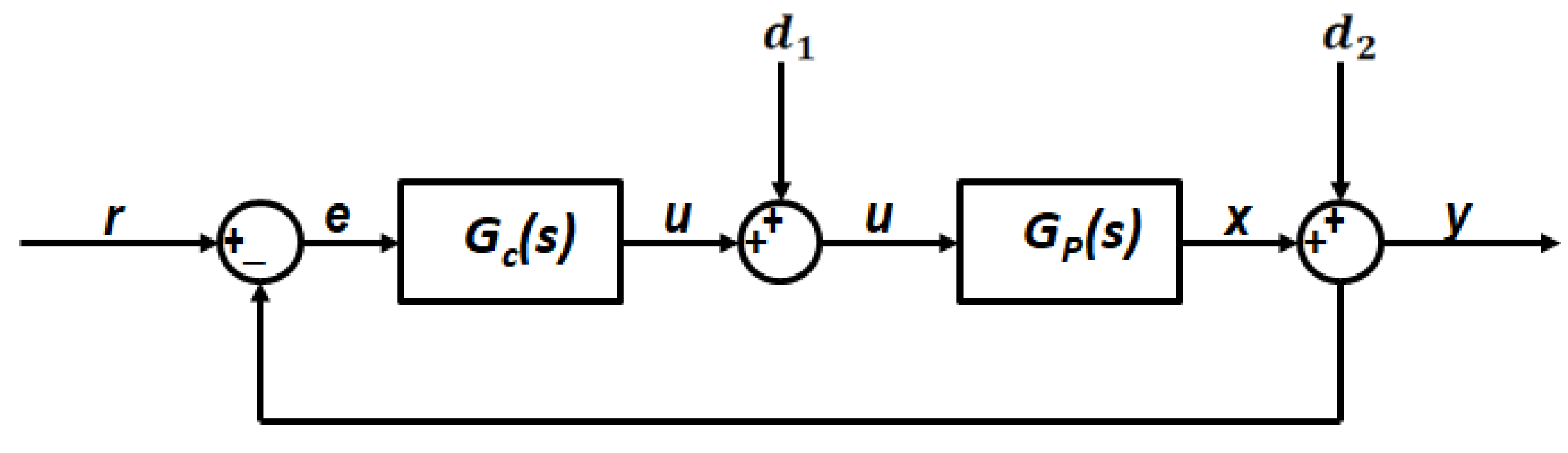
Moreover, for simplicity, the control system feedback is assumed to be restricted to operate on the error signal only. This includes the ability to follow reference signals, effects of load disturbances, and measurement noise (Åström [134]). The effects of process variations are not discussed here. For linear systems, the properties are captured by a set of four transfer functions. This is in addition to the system open-loop transfer function, which is needed in control system analysis. The transfer functions can be inspected in different ways, by their step responses or frequency responses. The following set of transfer functions was used in the present analysis:
- ▪
- Open-loop transfer function which defined by
- ▪
- Closed-loop system reference tracking (from r to y), which is called the complementary sensitivity function:
- ▪
- Closed-loop system noise sensitivity function used for controller action (effort) calculations due to limitations caused by practical constraints, such as controller saturation (from r to y),
- ▪
- Closed-loop system response to a load disturbance (for a step disturbance at the plant input,) (from to y), which is called the load disturbance sensitivity functionand
- ▪
- Closed-loop system response to a step disturbance at plant output, .which is called the sensitivity function (from to y)
The basic difference between input and output disturbances is that the input disturbance is generated in actuator while the output disturbance is generated in the sensor. For obtaining the time-domain characteristics of the control systems, frequently the step response, impulse response, and ramp response are evaluated. Transient characteristics such as peak time, settling time, rise time, maximum overshoot can be determined by evaluating the step response of the system.
References
- Gad-El-Hak, M. Flow Control: The Future. J. Aircr. 2001, 38, 402–418. [Google Scholar] [CrossRef]
- Simpson, R.L. Turbulent Boundary-Layer Separation. Annu. Rev. Fluid Mech. 1998, 21, 205–232. [Google Scholar] [CrossRef]
- Benard, N.; Cattafesta, L.N.; Moreau, E.; Griffin, J.; Bonnet, J.-P. On the benefits of hysteresis effects for closed-loop separation control using plasma actuation. Phys. Fluids 2011, 23, 083601. [Google Scholar] [CrossRef]
- Mabe, J.H.; Calkins, F.T.; Wesley, B.; Woszidlo, R.; Taubert, L.; Wygnanski, I. Single Dielectric Barrier Discharge Plasma Actuators for Improved Airfoil Performance. J. Aircr. 2009, 46, 847–855. [Google Scholar] [CrossRef]
- Huebsch, W.W.; Gall, P.D.; Hamburg, S.; Rothmayer, A.P. Dynamic Roughness as a Means of Leading-Edge Separation Flow Control. J. Aircr. 2012, 49, 108–115. [Google Scholar] [CrossRef]
- Schrauf, G. Application of Laminar Flow Technology on Transport Aircraft. In Proceedings of the CEAS Drag Reduction Conference, Potsdam, Germany, 3–5 June 2000; pp. 19–21. Available online: https://ntrs.nasa.gov/search.jsp?R=19780019127-2020-01-26T01:38:49+00:00Z (accessed on 17 May 2019).
- Joslin, R.D.; Miller, D.N. (Eds.) Fundamentals and Applications of Modern Flow Control; American Institute of Aeronautics and Astronautics (AIAA): Reston, VA, USA, 2009; Volume 231, pp. 1–20. [Google Scholar] [CrossRef]
- Cattafesta, L.; Song, Q.; Williams, D.R.; Rowley, C.W.; Alvi, F.S. Active control of flow-induced cavity oscillations. Prog. Aerosp. Sci. 2008, 44, 479–502. [Google Scholar] [CrossRef]
- Williams, D.R.; MacMynowski, D. Brief History of Flow Control Fundamentals and Applications of Modern Flow Control; AIAA: Reston, VA, USA, 2008; Chapter 1; pp. 1–20. [Google Scholar] [CrossRef]
- Bechert, D.W.; Bruse, M.; Hage, W.; Van Der Hoeven, J.T.; Hoppe, G. Experiments on drag-reducing surfaces and their optimization with an adjustable geometry. J. Fluid Mech. 1997, 338, 59–87. [Google Scholar] [CrossRef]
- Fisher, D.; Cobleigh, B.; Banks, D.; Hall, R.; Wahls, R. Reynolds number effects at high angles of attack. In Proceedings of the 20th AIAA Advanced Measurement and Ground Testing Technology Conference, Albuquerque, NM, USA, 15–18 June 1998. [Google Scholar] [CrossRef] [Green Version]
- Kaplanski, F.; Kartushinsky, A.; Hussainov, M.; Rudi, U.; Konhen, G.; Rüger, M. Some Experimental and Numerical Investigations of Flow near the Riblet Surfaces. In Proceedings of the 9th Workshop on Two-phase Flow Predictions, Merseburg, Germany, 13–16 April 1999; pp. 226–231. Available online: https://wwwresearchgate.net/publication/278242403 (accessed on 12 August 2019).
- Kaplanski, F.; Hussainov, M.; Kartushinsky, A.; Rudi, Ü. Flow near the Hemispherical Depressions. J. Mech. Behav. Mater. 2000, 11, 407–417. [Google Scholar] [CrossRef]
- Hussainov, M.; Kartushinsky, A.; Rudi, Ü.; Shcheglov, I.; Kohnen, G.; Sommerfeld, M. Experimental investigation of turbulence modulation by solid particles in a grid-generated vertical flow. Int. J. Heat Fluid Flow 2000, 21, 365–373. [Google Scholar] [CrossRef]
- Hussainov, M.; Kartushinsky, A.; Rudi, U.; Shcheglov, I.; Tisler, S. Experimental Study of the Effect of Velocity Slip and Mass Loading on the Modification of Grid-Generated Turbulence in Gas-Solid Particles Flows. Proc. Estonian Acad. Sci. Eng. 2005, 11, 169–180. [Google Scholar]
- Noack, B.; Morzyński, M.; Tadmor, G. Reduced Order Modeling for Flow Control; Springer Wien New York: Udine, Italy, 2011; Available online: https://www.springerprofessional.de/en/reduced-order-modelling-for-flow-control/4427676 (accessed on 8 February 2019).
- Bushnell, D.M. Turbulence Sensitivity and Control in Wall Flows. In Theoretical Approaches to Turbulence; Springer: New York, NY, USA, 1985. [Google Scholar] [CrossRef]
- Lumley, J.; Blossey, P. Control of Turbulence. Annu. Rev. Fluid Mech. 1998, 30, 311–327. [Google Scholar] [CrossRef]
- Cattafesta, L.; Sheplack, M. Actuators and Sensors. In Fundamentals and Applications of Modern Flow Control; AIAA: Reston, VA, USA, 2008; Chapter 6; pp. 149–176. [Google Scholar] [CrossRef]
- Mathew, J.; Song, Q.; Sankar, B.; Sheplak, M.; Cattafesta, L.N., III. Optimized Design of Piezoelectric Flap Actuators for Active Flow Control. AIAA J. 2006, 44, 2919–2928. [Google Scholar] [CrossRef]
- Wong, C.; Kontis, K. Flow Control by Spanwise Blowing on a NACA 0012. J. Aircr. 2007, 44, 337–340. [Google Scholar] [CrossRef]
- Eldredge, R.; Bons, J. Active Control of a Separating Boundary Layer with Steady Vortex Generating Jets–Detailed Flow Measurements. In Proceedings of the 42nd AIAA Aerospace Sciences Meeting and Exhibit, Reno, NV, USA, 5–8 January 2004. [Google Scholar] [CrossRef]
- Shan, H.; Jiang, L.; Liu, C.; Love, M.; Maines, B. Numerical study of passive and active flow separation control over a NACA0012 airfoil. Comput. Fluids 2008, 37, 975–992. [Google Scholar] [CrossRef]
- Seifert, A.; Greenblatt, D.; Wygnanski, I.J. Active separation control: An overview of Reynolds and Mach numbers effects. Aerosp. Sci. Technol. 2004, 8, 569–582. [Google Scholar] [CrossRef]
- Amitay, M.; Glezer, A. Controlled transients of flow reattachment over stalled airfoils. Int. J. Heat Fluid Flow 2002, 23, 690–699. [Google Scholar] [CrossRef]
- Seifert, A.; Darabi, A.; Wyganski, I. Delay of airfoil stall by periodic excitation. J. Aircr. 1996, 33, 691–698. [Google Scholar] [CrossRef]
- Billings, S.A.; Leontaritis, I.J. Parameter Estimation Techniques for Non-linear Systems. In Proceedings of the 6th IFAC Symposium on System Identification and Parameter Estimation, Washington, DC, USA, 7–11 June 1982; pp. 505–510. [Google Scholar] [CrossRef]
- Nishizawa, A.; Takagi, S.; Abe, H.; Kikushima, Y.; Maeda, R.; Yoshida, H. Toward Smart Control of Separation around Wing-part 1. In Proceedings of the 5th Symposium of Smart Control of Turbulence, Tokyo, Japan, 2–5 March 2005. [Google Scholar] [CrossRef]
- Nishizawa, A.; Takagi, S.; Abe, H.; Segawa, T.; Yoshida, H. Smart Control of Separation around a Wing–Control System. In Proceedings of the 6th Symposium of Smart Control of Turbulence, Tokyo, Japan, 6–9 March 2005; pp. 1–8. Available online: https://www.nmri.go.jp/oldpages/turbulence/PDF/symposium/FY2003/Nishizawa.pdf (accessed on 15 January 2020).
- Abe, H.; Segawa, T.; Kikushima, Y.; Pang, J.; Yoshida, H.; Nishizawa, A.; Takagi, S. Smart Control of Separation around a Wing—Control Device. In Proceedings of the 6th Symposium, Smart Control of Turbulence, Tokyo, Japan, 2–5 March 2005; Available online: https://www.nmri.go.Jp/oldpages2/turbulence/PDF/symposium/FY2004/Abe.pdf (accessed on 15 January 2020).
- Segawa, T.; Yoshida, H.; Nishizawa, A.; Murakami, K.; Mizunuma, H. Sensors and Actuators for Smart Control of Separation. In Proceedings of the Theoretical and Applied Mechanics, Tokyo Japan, 12–17 March 2003; Volume 52, pp. 117–125. Available online: https://www.jstage.jst.go.jp/article/nctam/52/0/52_0_117/_article/-char/ja (accessed on 2 January 2020).
- Tian, Y.; Cattafesta, L.; Mittal, R. Adaptive Control of Separated Flow. In Proceedings of the 44th AIAA Aerospace Sciences Meeting and Exhibit, Reno, NV, USA, 9–12 January 2006; pp. 1401–1411. [Google Scholar] [CrossRef] [Green Version]
- Tian, Y.; Song, Q.; Cattafesta, L. Adaptive Feedback Control of Flow Separation. In Proceedings of the 3rd AIAA Flow Control Conference, San Francisco, CA, USA, 5–8 June 2006. [Google Scholar] [CrossRef] [Green Version]
- Song, Q.; Tian, Y.; Cattafesta, L. MIMO Feedback Control of Flow Separation. In Proceedings of the 45th AIAA Aerospace Sciences Meeting and Exhibit, Reno, NV, USA, 8–11 January 2007. [Google Scholar] [CrossRef]
- Pinier, J.; Ausseur, J.M.; Glauser, M.N.; Higuchi, H. Proportional Closed-Loop Feedback Control of Flow Separation. AIAA J. 2007, 45, 181–190. [Google Scholar] [CrossRef]
- Ausseur, J.; Pinier, J.; Glauser, M. Estimation Techniques in a Turbulent Flow Field. In Proceedings of the 37th AIAA Fluid Dynamics Conference and Exhibit, Miami, FL, USA, 25–28 June 2007; Available online: https://www.researchgate.net/publication/259676298 (accessed on 19 December 2019).
- Becker, R.; King, R.; Petz, R.; Nitsche, W. Adaptive Closed-Loop Separation Control on a High-Lift Configuration Using Extremum Seeking. AIAA J. 2007, 45, 1382–1392. [Google Scholar] [CrossRef]
- Allan, B.; Juang, J.; Raney, D.; Seifert, A.; Pack, L.; Brown, D. Closed-Loop Separation Control Using Oscillatory Flow Excitation; NACA/CR, Technical Report; NACA Langley Research Center: Hampton, VA, USA, 2000; pp. 1–24. Available online: https://www.researchgate.net/publication/24301862 (accessed on 2 January 2020).
- Becker, R.; Garwon, M.; Gutknecht, C.; Bärwolff, G.; King, R. Robust control of separated shear flows in simulation and experiment. J. Process. Control. 2005, 15, 691–700. [Google Scholar] [CrossRef]
- Henning, L.; King, R. Multivariable Closed-Loop Control of the Reattachment Length Downstream of a Backward-Facing Step. In Proceedings of the 16th International IFAC World Congress, Praha, Czech Republic, 4–8 July 2005. [Google Scholar] [CrossRef]
- Becker, R.; King, R. Comparison of a robust and a flatness based control for a separated shear flow. In Proceedings of the 16th International IFAC World Congress, Praha, Czech Republic, 4–8 July 2005. [Google Scholar] [CrossRef]
- Duvigneau, R.; Visonneau, M. Optimization of a synthetic jet actuator for aerodynamic stall control. Comput. Fluids 2006, 35, 624–638. [Google Scholar] [CrossRef] [Green Version]
- Bourgois, P.R. Closed-Loop Proportional Controller for Flow Separation on ONERA Airfoil; CNRS UMR 7128; ONERA Publications: Toulouse, France, 2009; pp. 1–34. Available online: https://www.imft.fr/IMG/pdf/liste_des_publications_2005_2009_imft.pdf (accessed on 2 March 2019).
- Cattafesta, L.; Tian, Y.; Mittal, R. Adaptive Control of Post-Stall Separated Flow Application to Heavy Vehicles. In The Aerodynamics of Heavy Vehicles II: Trucks, Buses, and Trains, Lecture Notes in Applied and Computational Mechanics Fracture Mechanics; Springer: Berlin/Heidelberg, Germany, 2009; Volume 41, pp. 151–160. Available online: https://www.researchgate.net/publication/227108242 (accessed on 2 March 2019).
- Cho, Y.C.; Fledderjohn, M.; Holzel, M.; Jayaraman, B.; Santillo, M.; Bernstein, D.S.; Shyy, W. Adaptive Flow Control of Low Reynolds Number Aerodynamics Using a Dielectric Barrier Discharge Actuator. In Proceedings of the 47th AIAA Aerospace Sciences Meeting Including The New Horizons Forum and Aerospace Exposition, Orlando, FL, USA, 5–8 January 2009. [Google Scholar] [CrossRef] [Green Version]
- Taira, K.; Rowley, C.W.; Colonius, T. Feedback Control of High-Lift State for a Low-Aspect-Ratio Wing. In Proceedings of the 48th AIAA Aerospace Sciences Meeting Including the New Horizons Forum and Aerospace Exposition, Orlando, FL, USA, 4–7 January 2010. [Google Scholar] [CrossRef] [Green Version]
- Benard, N.; Moreau, E.; Griffin, J.; Iii, L.N.C. Slope seeking for autonomous lift improvement by plasma surface discharge. Exp. Fluids 2009, 48, 791–808. [Google Scholar] [CrossRef]
- Luchtenburg, D.M.; Aleksić, K.; Schlegel, M.; Noack, B.R.; King, R.; Tadmor, G.; Günther, B.; Thiele, F. Turbulence Control Based on Reduced-Order Models and Nonlinear Control Design. In Active Flow Control II; King, R., Ed.; Springer: Berlin/Heidelberg, Germany, 2010; pp. 341–356. [Google Scholar] [CrossRef]
- Colonius, T.; Williams, D.R. Control of vortex shedding on two-and three-dimensional aerofoils. Philos. Trans. R. Soc. Math. Phys. Eng. Sci. 2011, 369, 1525–1539. [Google Scholar] [CrossRef] [PubMed] [Green Version]
- Tuck, A.; Soria, J. Separation control on a NACA 0015 airfoil using a 2D micro ZNMF jet. Aircr. Eng. Aerosp. Technol. 2008, 80, 175–180. [Google Scholar] [CrossRef]
- Amitay, M.; Glezer, A. Role of Actuation Frequency in Controlled Flow Reattachment over a Stalled Airfoil. AIAA J. 2002, 40, 209–216. [Google Scholar] [CrossRef]
- He, Y.; Cary, A.; Peters, D. Parametric and dynamic modeling for synthetic jet control of a post-stall airfoil. In Proceedings of the 39th Aerospace Sciences Meeting and Exhibit, Reno, NV, USA, 8–11 January 2001. [Google Scholar] [CrossRef]
- Amitay, M.; Kibens, V.; Parekh, D.; Glezer, A. The dynamics of flow reattachment over a thick airfoil controlled by synthetic jet actuators. In Proceedings of the 37th Aerospace Sciences Meeting and Exhibit, Reno, NV, USA, 11–14 January 1999. [Google Scholar] [CrossRef]
- Crook, A.; Sadri, A.; Wood, N. The development and implementation of synthetic jets for the control of separated flow. In Proceedings of the 17th Applied Aerodynamics Conference, Norfolk, VA, USA, 28 June–1 July 1999. [Google Scholar] [CrossRef]
- Seifert, A.; Pack, L. Oscillatory excitation of unsteady compressible flows over airfoils at flight Reynolds numbers. In Proceedings of the 37th Aerospace Sciences Meeting and Exhibit, Reno, NV, USA, 11–14 January 1999. [Google Scholar] [CrossRef] [Green Version]
- Amitay, M.; Smith, D.; Kibens, V.; Parekh, D.; Glezer, A. Aerodynamic Flow Control of Bluff Bodies Using Synthetic Jet Actuators. In Proceedings of the IUTAM Symposium on Mechanics of Passive and Active Control, Gottingen, Germany, 7–11 September 1998; Available online: https://link.springer.com/chapter/10.1007/978-94-011-4199444 (accessed on 19 December 2019).
- Smith, D.; Amitay, M.; Kibens, V.; Parekh, D.; Glezer, A. Modification of lifting body aerodynamics using synthetic jet actuators. In Proceedings of the 36th AIAA Aerospace Sciences Meeting and Exhibit, Reno, NV, USA, 12–15 January 1998. [Google Scholar] [CrossRef]
- Amitay, M.; Pitt, D.; Glezer, A. Separation Control in Duct Flows. J. Aircr. 2002, 39, 616–620. [Google Scholar] [CrossRef]
- Parekh, D.; Williams, S.; Amitay, M.; Glezer, A.; Washburn, T.; Gregory, I.; Scott, R. Synthetic Jet Aerodynamic Control on a Full Scale UAV. In Proceedings of the 33rd AIAA Fluid Dynamics Conference and Exhibit, Orlando, FL, USA, 23–26 June 2003. [Google Scholar] [CrossRef]
- Ciuryla, M.; Liu, Y.; Farnsworth, J.; Kwan, C.; Amitay, M. Flight Control Using Synthetic Jets on a Cessna 182 Model. J. Aircr. 2007, 44, 642–653. [Google Scholar] [CrossRef]
- Smith, B.L.; Glezer, A. Jet vectoring using synthetic jets. J. Fluid Mech. 2002, 458, 1–34. [Google Scholar] [CrossRef]
- Maldonado, V.; Farnsworth, J.; Gressick, W.; Amitay, M. Active control of flow separation and structural vibrations of wind turbine blades. Wind. Energy 2010, 13, 221–237. [Google Scholar] [CrossRef]
- Chatlynne, E.; Rumigny, N.; Amitay, M.; Glezer, A. Virtual aero-shaping of a Clark-Y airfoil using synthetic jet actuators. In Proceedings of the 39th Aerospace Sciences Meeting and Exhibit, Reno, NV, USA, 8–11 January 2001. [Google Scholar] [CrossRef]
- Amitay, M.; Horvath, M.; Michaux, M.; Glezer, A. Virtual aerodynamic shape modification at low angles of attack using synthetic jet actuators. In Proceedings of the 15th AIAA Computational Fluid Dynamics Conference, Anaheim, CA, USA, 11–14 June 2001. [Google Scholar] [CrossRef]
- Farnsworth, J.A.N.; Vaccaro, J.C.; Amitay, M. Active Flow Control at Low Angles of Attack: Stingray Unmanned Aerial Vehicle. AIAA J. 2008, 46, 2530–2544. [Google Scholar] [CrossRef]
- Timor, I.; Ben-Hamou, E.; Guy, Y.; Seifert, A. Maneuvering Aspects and 3D Effects of Active Airfoil Flow Control. Flow Turbul. Combust. 2007, 78, 429–443. [Google Scholar] [CrossRef]
- Darabi, A.; Wygnanski, I. Active Management of Naturally Separated Flow over a Solid Surface. Part 1: The forced reattachment process. J. Fluid Mech. 2004, 510, 105–129. [Google Scholar] [CrossRef]
- Darabi, A.; Wygnanski, I. Active Management of Naturally Separated Flow over a Solid Surface. Part 2: The Separation Process. J. Fluid Mech. 2004, 510, 131–144. [Google Scholar] [CrossRef]
- Amitay, M.; Glezer, A. Flow transients induced on a 2D airfoil by pulse-modulated actuation. Exp. Fluids 2005, 40, 329–331. [Google Scholar] [CrossRef]
- Mathis, R.; Lebedev, A.; Collin, E.; Delville, J.; Bonnet, J.-P. Experimental study of transient forced turbulent separation and reattachment on a bevelled trailing edge. Exp. Fluids 2008, 46, 131–146. [Google Scholar] [CrossRef]
- Jones, D.A.; Clarke, D.B. Simulation of Flow Past a Sphere Using the Fluent Code; Maritime Platforms Division: Fishermans Bend, Australia, 2008; pp. 1–35. Available online: https://pdfs.Semanticscholar.org/34cf/df61323f0c871e3c97e7cbce1e1f7dbef00e.pdf (accessed on 2 March 2019).
- Slotnick, J.; Khodadoust, A.; Alonso, J.; Darmofal, D.; Gropp, W.; Lurie, E.; Mavriplis, D. CFD Vision 2030 Study: A Path to Revolutionary Computational Aerosciences; NASA Langley Research Center: Hampton, VA, USA, 2014; pp. 1–58. Available online: https://ntrs.nasa.gov/search.jsp?R=20140003093 (accessed on 2 March 2019).
- Choi, H.; Moin, P.; Kim, J. Active turbulence control for drag reduction in wall-bounded flows. J. Fluid Mech. 1994, 262, 75. [Google Scholar] [CrossRef]
- Kim, J. Control of turbulent boundary layers. Phys. Fluids 2003, 15, 1093–1105. [Google Scholar] [CrossRef]
- Banaszuk, A.; Naraynan, S.; Zhang, Y. Adaptive Control of Flow Separation in a Planar Diffuser. In Proceedings of the 41st Aerospace Sciences Meeting and Exhibit, Reno, Nevada, 6–9 January 2003. [Google Scholar] [CrossRef]
- Chen, S.; Billings, S.A. Representation of Non-linear Systems: The NARMAX Model. Int. J. Control 1989, 49, 1013–1032. Available online: http://eprints.soton.ac.uk/id/eprint/251145 (accessed on 27 December 2019).
- Billings, S.A. Nonlinear System Identification, NARMAX Methods in the Time, Frequency, and Spatio-Temporal Domains; John Wiley & Sons: Hoboken, NJ, USA, 2013; ISBN 978-1-119-94359-4. Available online: https://www.wiley.com/en-us/exportProduct/pdf/9781119943594 (accessed on 4 January 2019).
- Liu, Y.P. Identification of Nonlinear Systems: The NARMAX Polynomial Model Approach. Ph.D. Thesis, University of Sheffield, Sheffield, UK, 1988. Available online: https://sheffield.libguides.com/guideacse/communicating (accessed on 4 January 2019).
- Leontaritis, I.J.; Billings, S.A. Input-output parametric models for non-linear systems Part II: Stochastic non-linear systems. Int. J. Control 1985, 41, 329–344. [Google Scholar] [CrossRef]
- Thomson, M.; Schooling, S.; Soufian, M. The practical application of a nonlinear identification methodology. Control. Eng. Pr. 1996, 4, 295–306. [Google Scholar] [CrossRef]
- Swain, A.; Billings, S.; Stansby, P.; Baker, M. Accurate prediction of non-linear wave forces: Part I (fixed cylinder). Mech. Syst. Signal Process. 1998, 12, 449–485. [Google Scholar] [CrossRef]
- Billings, S.; Stansby, P.; Swain, A.; Baker, M. Accurate Prediction of Non-Linear Wave Forces: Part II (Responding Cylinder). Mech. Syst. Signal Process. 1998, 12, 487–498. [Google Scholar] [CrossRef]
- Kukreja, S.L.; Brenner, M.J. Nonlinear System Identification of Aero-elastic Systems: A Structure-detection Approach. In Identification and Control; Part II; Springer: London, UK, 2007; pp. 117–145. [Google Scholar] [CrossRef]
- Ching, S.; Eun, Y.; Kabamba, P.T.; Meerkov, S.M. Quasilinear Control Theory: An Overview. In Proceedings of the 18th IFAC World Congress, Milano, Italy, 28 August–2 September 2011. [Google Scholar] [CrossRef] [Green Version]
- Wu, J.M.; Lu, X.Y.; Denney, A.G.; Fan, M.; Wu, J.Z. Post-stall Lift Enhancement on an Airfoil by Local Unsteady Control Part I, Lift, Drag and Pressure Characteristics. In Proceedings of the 4th Shear Flow Control Conference, Snowmass Village, CO, USA, 29 June–2 July 1997; Available online: http://staff.ustc.edu.cn/~xlu/download/JFM_1998.pdf (accessed on 27 December 2019).
- Abbott Ira, H.; Von Doenhoff, A.E. Theory of Wing Sections: Including a Summary of Airfoil Data (Dover Books on Aeronautical Engineering); Courier Corporation: North Chelmsford, MA, USA, March 1959; pp. 324–390. ISBN 978-0486605869. Available online: https://aeroknowledge77.files.wordpress.com/2011/09/589-86488-theory-of-wing-sections-including-a-summary-of-airfoil-data.pdf (accessed on 1 February 2020).
- Dolle, T.J.A. Flap Performance Improvement by Surface Excitation. Master’s Thesis, Aerospace Engineering at Delft University of Technology, Mekelweg, The Netherlands, 2009; pp. 1–144. Available online: http://resolver.tudelft.nl/uuid:985ea160-f12c-472f-9670-fd8ad333ee64 (accessed on 27 December 2019).
- Duvigneau, R.; Visonneau, M. Simulation and optimization of stall control for an airfoil with a synthetic jet. Aerosp. Sci. Technol. 2006, 10, 279–287. [Google Scholar] [CrossRef] [Green Version]
- Anderson, W.; Bonhaus, D.L. An implicit upwind algorithm for computing turbulent flows on unstructured grids. Comput. Fluids 1994, 23, 1–21. [Google Scholar] [CrossRef] [Green Version]
- Bakker, A. Solution Methods Applied Computational Fluid Dynamics. In Lectures of Fluent Instructor; Lecture 5Fluent Inc.: New York, NY, USA, 2002; pp. 1–45. Available online: http://www.bakker.org/dartmouth06/engs150/05-solv.pdf (accessed on 7 January 2020).
- Obeid, S.; Jha, R.; Ahmadi, G. RANS Simulations of Aerodynamic Performance of NACA 0015 Flapped Airfoil. Fluids 2017, 2, 2. [Google Scholar] [CrossRef] [Green Version]
- Rethmel, C.C. Airfoil Leading Edge Flow Separation Control Using Nano-second Pulse DBD Plasma Actuators. Master’s Thesis, The Ohio State University, Columbus, OH, USA, May 2011; pp. 1–80. Available online: http://rave.ohiolink.edu/etdc/view?acc_num=osu1306348260 (accessed on 27 December 2019).
- You, D.; Moin, P. Active control of flow separation over an airfoil using synthetic jets. J. Fluids Struct. 2008, 24, 1349–1357. [Google Scholar] [CrossRef]
- Joseph, D.D.; Liao, T.Y. Potential flows of viscous and viscoelastic fluids. J. Fluid Mech. 1994, 265, 1–23. [Google Scholar] [CrossRef] [Green Version]
- Schroeder, E.J. Low Reynolds Number Flow Validation Using Computational Fluid Dynamics with Application to Micro Air Vehicles. Master’s Thesis, University of Maryland, College Park, MD, USA, 2005; pp. 20–23. Available online: https://drum.lib.umd.edu/handle/1903/3349 (accessed on 2 March 2019).
- Manni, L.; Nishino, T.; Delafin, P.-L. Numerical study of airfoil stall cells using a very wide computational domain. Comput. Fluids 2016, 140, 260–269. [Google Scholar] [CrossRef] [Green Version]
- Sharma, D.M. Experimental Investigations of Dynamic Stall for an Oscillating Airfoil. Ph.D. Thesis, Aeronautical Engineering, Indian Institute of Technology Kanpur, Kanpur, India, 2010; pp. 90–102. [Google Scholar] [CrossRef]
- Rediniotis, O.K. Synthetic Jet Actuation—Modeling, Actuator Development and Application to Separation Control; Texas Engineering Experiment College Station, Texas A&M University: College Station, TX, USA, 2004. Available online: https://apps.dticmil/dtic/tr/fulltext/u2/a424008.pdf (accessed on 4 February 2020).
- Billings, S.A.; Leontaritis, I.J. Identification of Non-Linear System Using Parameter Estimation. In Proceedings of the 6th IFAC Symposium on Identification and System Parameter Estimation, Washington, DC, USA, 7–11 June 1982; Volumes 15, pp. 505–510. Available online: https://www.sciencedirect.com/journal/ifac-proceedings-volumes/vol/15/issue/4 (accessed on 10 October 2019).
- Leontaritis, I.J.; Billings, S.A. Input-output parametric models for non-linear systems Part I: Deterministic non-linear systems. Int. J. Control 1985, 41, 303–328. [Google Scholar] [CrossRef]
- Chiras, N.; Evans, C.; Rees, D. Nonlinear gas turbine computer modelling using NARMAX structures. In Proceedings of the 17th IEEE Instrumentation and Measurement Technology Conference, Baltimore, MD, USA, 1–4 May 2000; pp. 1278–1284. [Google Scholar] [CrossRef]
- Billings, S.A.; Chen, S. Extended model set, global data and threshold model identification of severely non-linear systems. Int. J. Control 1989, 50, 1897–1923. [Google Scholar] [CrossRef]
- Aguirre, L.A.; Billings, S.A. Improved structure selection for nonlinear models based on term clustering. Int. J. Control 1995, 62, 569–587. [Google Scholar] [CrossRef]
- Billings, S.A.; Aguirre, L.A. Effects of the Sampling Time on the Dynamics and Identification of Nonlinear Models. Int. J. Bifurc. Chaos 1995, 5, 1541–1556. [Google Scholar] [CrossRef]
- Akaike, H. A new look at the statistical model identification. IEEE Trans. Autom. Control 1974, 19, 716–723. [Google Scholar] [CrossRef]
- Nash, J.E.; Sutcliffe, J.V. River Flow Forecasting through Conceptual Models. J. Hydraul. 1970, 10, 282–290. [Google Scholar] [CrossRef]
- Mittal, R.; Kotapati, R.B. Resonant Mode Interaction in a Canonical Separated Flow. In Proceedings of the Sixth IUTAM Symposium on Laminar-Turbulent Transitions, Bangalore, India, 11–15 June 2006; Volume 78, pp. 341–348. [Google Scholar] [CrossRef]
- Ho, C.; Huerre, P. Perturbed Free Shear Layers. Annu. Rev. Fluid Mech. 1984, 16, 365–422. [Google Scholar] [CrossRef]
- Wu, J.-Z.; Lu, X.-Y.; Denny, A.G.; Fan, M.; Wu, J.-M. Post-stall flow control on an airfoil by local unsteady forcing. J. Fluid Mech. 1998, 371, 21–58. [Google Scholar] [CrossRef] [Green Version]
- Kim, K. Feedback Control of FlowFlow Separation Using Synthetic Jets. Ph.D. Thesis, Texas A&M University, Bizzell St, TX, USA, December 2005; pp. 1–187. Available online: https//etd-tamu-2005C-MEEN-Kim.pdf (accessed on 27 December 2019).
- Lavoie, P. Control of Separated Flows. Available online: http://arrow.utias.utoronto.ca/crsa/sssa/2016/lavoie.phil-UTIAS-separation.control-2016sssa.pdf (accessed on 14 February 2020).
- Maldonado, V.; Farnsworth, J.; Gressick, W.; Amitay, M. Active Enhancement of Wind Turbine Blades Performance. In Proceedings of the 46th AIAA Aerospace Sciences Meeting and Exhibit, Reno, NV, USA, 7–10 January 2008. [Google Scholar] [CrossRef]
- Benard, N.; Moreau, E. Capabilities of the dielectric barrier discharge plasma actuator for multi-frequency excitations. J. Phys. D Appl. Phys. 2010, 43, 145201. [Google Scholar] [CrossRef] [Green Version]
- Glezer, A.; Amitay, M. Syntheticjets. Annu. Rev. Fluid Mech. 2002, 34, 503–529. [Google Scholar] [CrossRef]
- Tang, H.; Zhong, S.; Jabbal, M.; Garcillan, L.; Guo, F.; Wood, N.; Warsop, C. Towards the Design of Synthetic-jet Actuators for Full-scale Flight Conditions. Flow Turbul. Combust. 2007, 78, 309–329. [Google Scholar] [CrossRef]
- Sharma, R.N. Some Insights into Synthetic Jet Actuation from Analytical Modelling. In Proceedings of the 16th Australasian Flu. Mechanics Conference, Gold Coast, Australia, 2–7 December 2007; pp. 1242–1248. Available online: https://people.eng.unimelb.edu.au/imarusic/proceedings/16/Sharma2.pdf (accessed on 11 August 2019).
- Kugelstadt, T. Active Filter Design Techniques. In Fundamentals of Low-Pass Filters Book; Texas Instruments: Dallas, TX, USA, March 2002; Chapter 16; pp. 1–66. Available online: https://www2.seas.gwu.edu/~ece121/Spring-11/filterdesign.pdf (accessed on 2 March 2019).
- Taylor, J.H.; Strobel, K.L. Applications of a Nonlinear Controller Design Approach based on Quasilinear System Models. In Proceedings of the 1984 American Control Conference, San Diego, CA, USA, 7–10 June 1984; pp. 817–824. [Google Scholar] [CrossRef]
- Taylor, J.H. Sinusoidal-Input Describing Function (SIDF). Available online: https://ocw.mit.edu/courses/aeronautics-and-astronautics/16-30-estimation-and-control-of-aerospace-systems-spring-2004/readings/gelb_ch2_ocr.pdf (accessed on 19 December 2019).
- Schwartz, C.; Gran, R. Describing function analysis using MATLAB and Simulink. IEEE Control. Syst. 2001, 21, 19–26. [Google Scholar] [CrossRef]
- Slotine, J.J.E.; Li, W. Applied Nonlinear Control; Prentice-Hall: Englewood Cliffs, NJ, USA, 1991; pp. 191–433. ISBN 0-13-040890-5. Available online: http://www.ioe.nchu.edu.tw/Pic/CourseItem/4497APPLIED%20NONLINEAR%20CONTROLslotine_Part1.pdf (accessed on 27 December 2019).
- Kim, K.; Kerr, M.; Beskok, A.; Jayasuriya, S. Frequency-domain based feedback control of flow separation using synthetic jets. In Proceedings of the American Control Conference, Minneapolis, MN, USA, 14–16 June 2006. [Google Scholar] [CrossRef]
- Vukic, Z.; Kuljaca, O. Lectures on PID Controllers; University of Texas: Arlington, TX, USA, 2002; pp. 5–41. Available online: http://www.uta.edu/utari/acs/jyotirmay/EE4343/Labs_Projects/pidcontrollers.pdf (accessed on 27 December 2019).
- Taylor, J.H. A General Limit Cycle Analysis Method for Multivariable Systems. In New Approaches to Nonlinear Problems in Dynamics; Holmes, P.J., Ed.; SIAM (Society of Industrial and Applied Mathematics): Philadelphia, PA, USA, 1980; ISBN 978-0898711677. Available online: https://trove.nla.gov.au/version/11860584 (accessed on 2 July 2019).
- Taylor, J.H. Describing Functions. In Electrical Engineering Encyclopedia; John Wiley & Sons, Inc.: New York, NY, USA, 1999. [Google Scholar] [CrossRef]
- Kotapati, R.B.; Mittal, R.; Marxen, O.; Ham, F.; You, D.; Cattafesta, L.N. Nonlinear dynamics and synthetic-jet-based control of a canonical separated flow. J. Fluid Mech. 2010, 654, 65–97. [Google Scholar] [CrossRef] [Green Version]
- Glass, J.W.; Franchek, M.A. Frequency-based nonlinear controller design for regulating systems subjected to time-domain constraints. Int. J. Robust Nonlinear Control 2000, 10, 39–57. [Google Scholar] [CrossRef]
- John, A. Understanding Bode Plots; Motion Engineering Inc. Notes: Santa Barbara, CA, USA, 2019; pp. 1–99. Available online: http://support.Motioneng.com/utilities/bode/bode_16.html (accessed on 2 January 2020).
- Shahzad, U. Design and Analysis of a Control System Using Root Locus and Frequency Response Methods. ITEE J. 2017, 6, 14–19. Available online: https://www.researchgate.net/publication/319653031 (accessed on 12 January 2020).
- Patino, D.; Riedinger, P.; Iung, C. Practical Optimal State Feedback Control Law for Continuous-Time Switched Affine Systems with Cyclic Steady State. Int. J. Control 2010, 82, 1251–1276. [Google Scholar] [CrossRef]
- Berk, Z. Elements of Process Control. In Food Process Engineering Technology; Science Dirt Elvester Book; Springer: New York, NY, USA, 2009; Chapter 5; pp. 129–151. Available online: https://www.sciencedirect.com/book/9780123736604/food-process-engineering-and-technology (accessed on 8 February 2020).
- Horowitz, I.M. Synthesis of Feedback Systems, 1st ed.; Elsevier: Amsterdam, The Netherlands, 1963; ISBN 9781 4 83267708. Available online: https://www.elsevier.com/books/synthesis-of-feedback-systems/horowitz/978-1-4832-3282-9 (accessed on 19 January 2020).
- Vandoren, V. Designing a Feedback Control Loop Starts with Understanding its Objective as well as the Process’s Behavior. Control Engineering Magazine. 7 March 2011, pp. 1–13. Available online: https://www.controleng.com/articles/disturbance-rejection-vs-setpoint-tracking-controllers (accessed on 23 December 2019).
- Åström, K.J. Control System Design. In Lecture Notes for ME 155A on Department of Mechanical Environmental Engineering; University of California: Santa Barbara, CA, USA, 2002; Available online: http://clux.x-pec.com/files/fronter/ENE103%20-%20Reguleringsteknikk/fagstoffsuplement%20Reg%20tek%20engelsk%20.pdf (accessed on 19 December 2019).
- MATLAB. Control System Tool Box, User’s Guide; The Math Works, Inc.: Natick, MA, USA, 2019; pp. 1–1815. Available online: https://www.mathworks.com/help/pdf_doc/control/index.html?s.cid=doc.ftr (accessed on 3 June 2019).
- Seborg, D.E.; Edgar, T.F.; Mellichamp, D.A.; Doyle, F.I., III. Process Dynamics and Control, 4th ed.; Johns Wiley & Sons: Hoboken, NJ, USA, 2017; Available online: https://www.wiley.com/en-us/Process.Dynamics.and.Control.4th.Edition-p-9781119285915 (accessed on 7 January 2020).
Figure 1.
URANS Simulation, schematic of the computational domain, airfoil location, and boundary conditions.
Figure 1.
URANS Simulation, schematic of the computational domain, airfoil location, and boundary conditions.
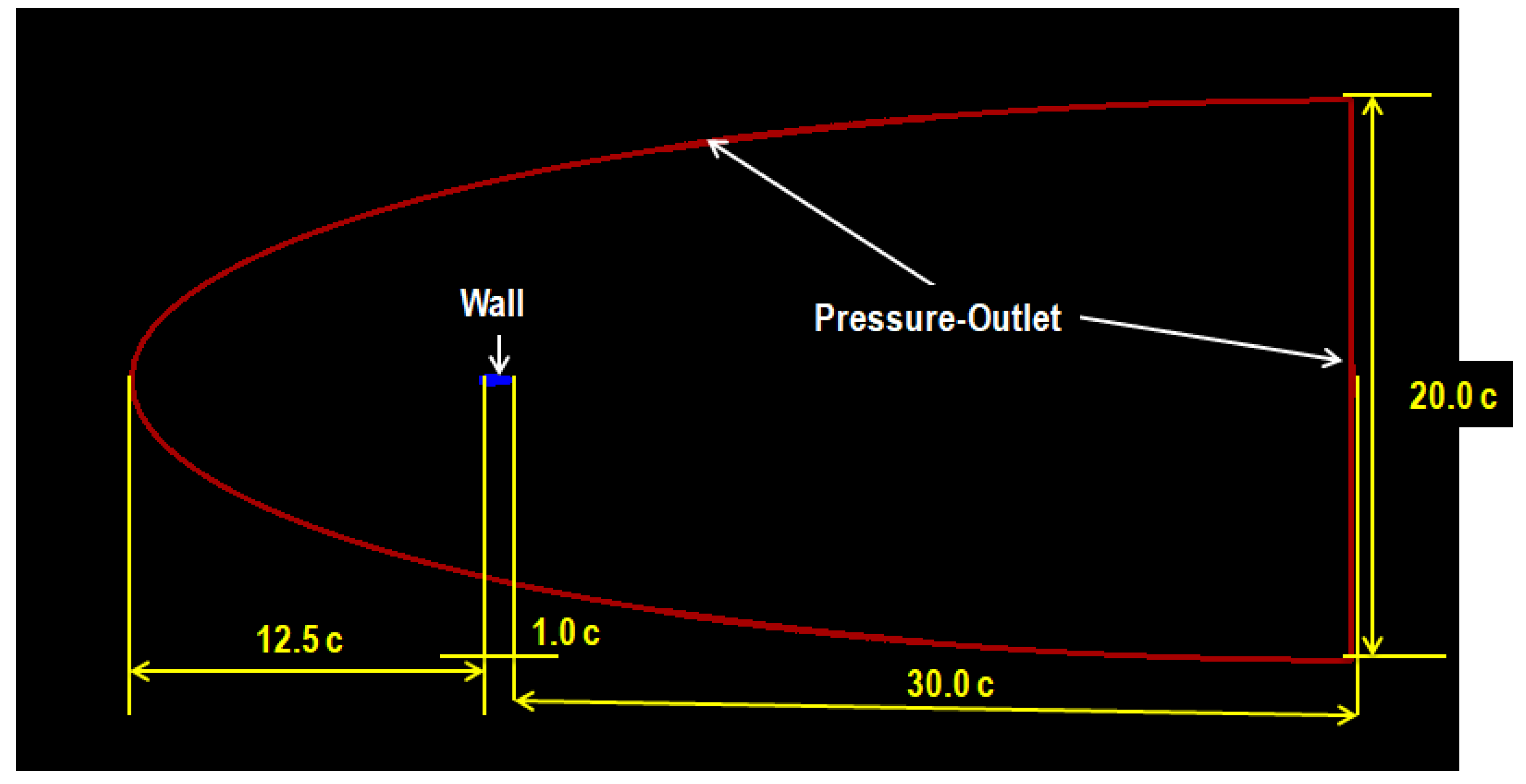
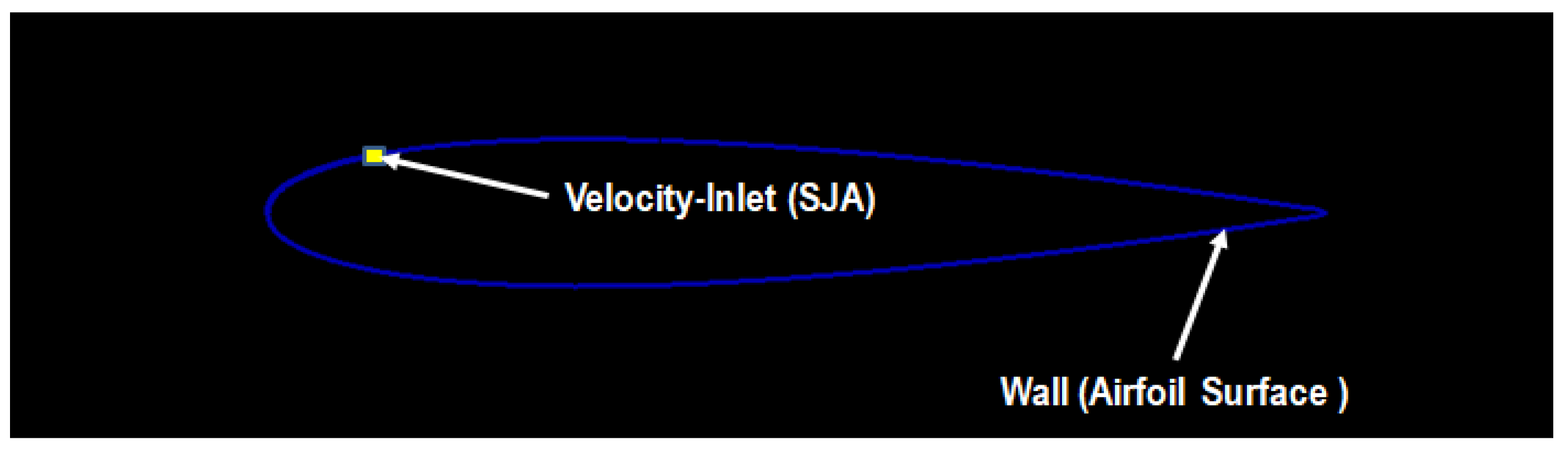
Figure 2.
Results of mesh intensity inspection for lift coefficient as predicted by the Spalart-Allmaras and the Realizable k-ε models at AoA = 12° for (a) Re = 105 and (b) Re =106.
Figure 2.
Results of mesh intensity inspection for lift coefficient as predicted by the Spalart-Allmaras and the Realizable k-ε models at AoA = 12° for (a) Re = 105 and (b) Re =106.
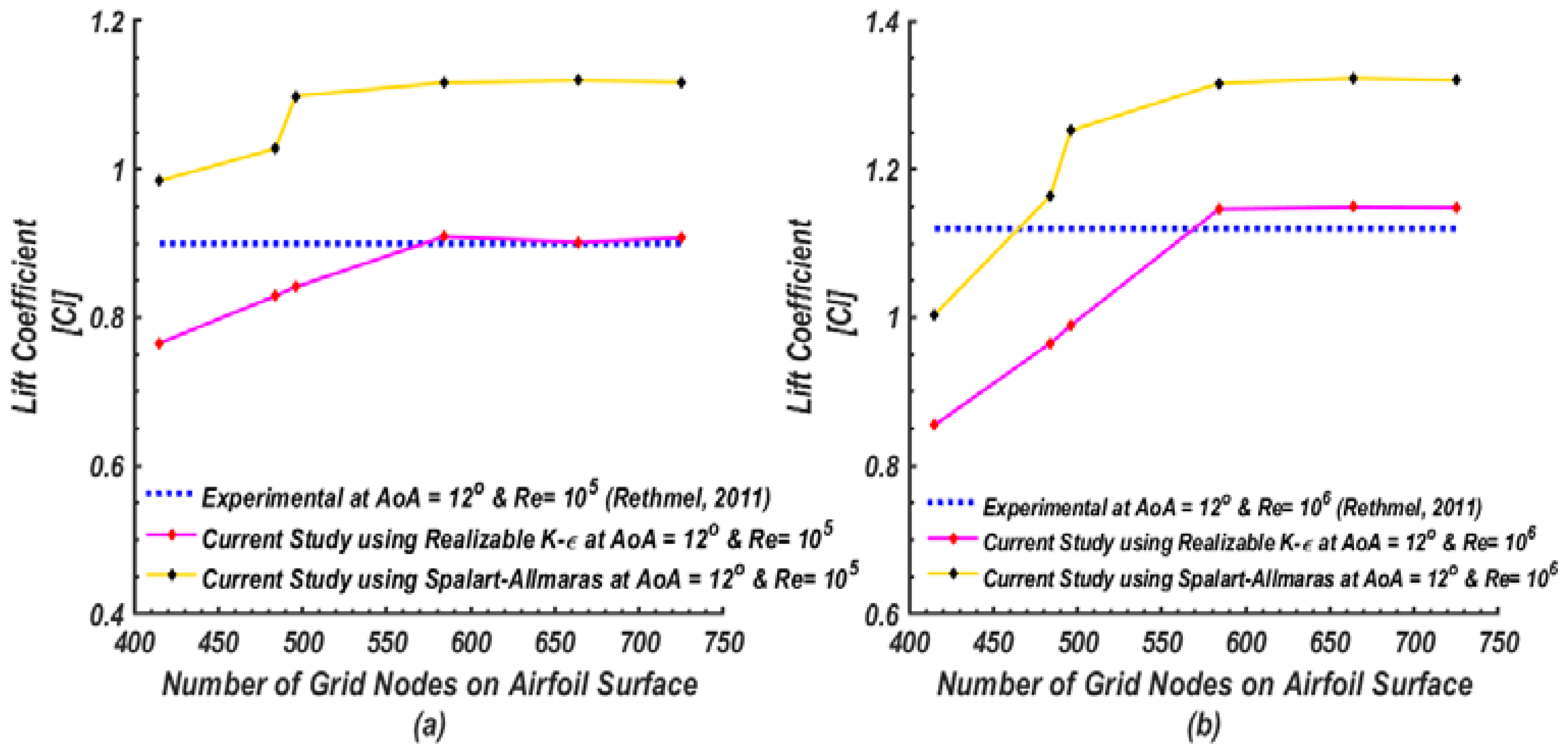
Figure 3.
Mesh structure for cases without SJA and with SJA, (a) Mesh clustering around airfoil surfaces, and (b) dense in the vicinity of the synthetic jet actuator.
Figure 3.
Mesh structure for cases without SJA and with SJA, (a) Mesh clustering around airfoil surfaces, and (b) dense in the vicinity of the synthetic jet actuator.
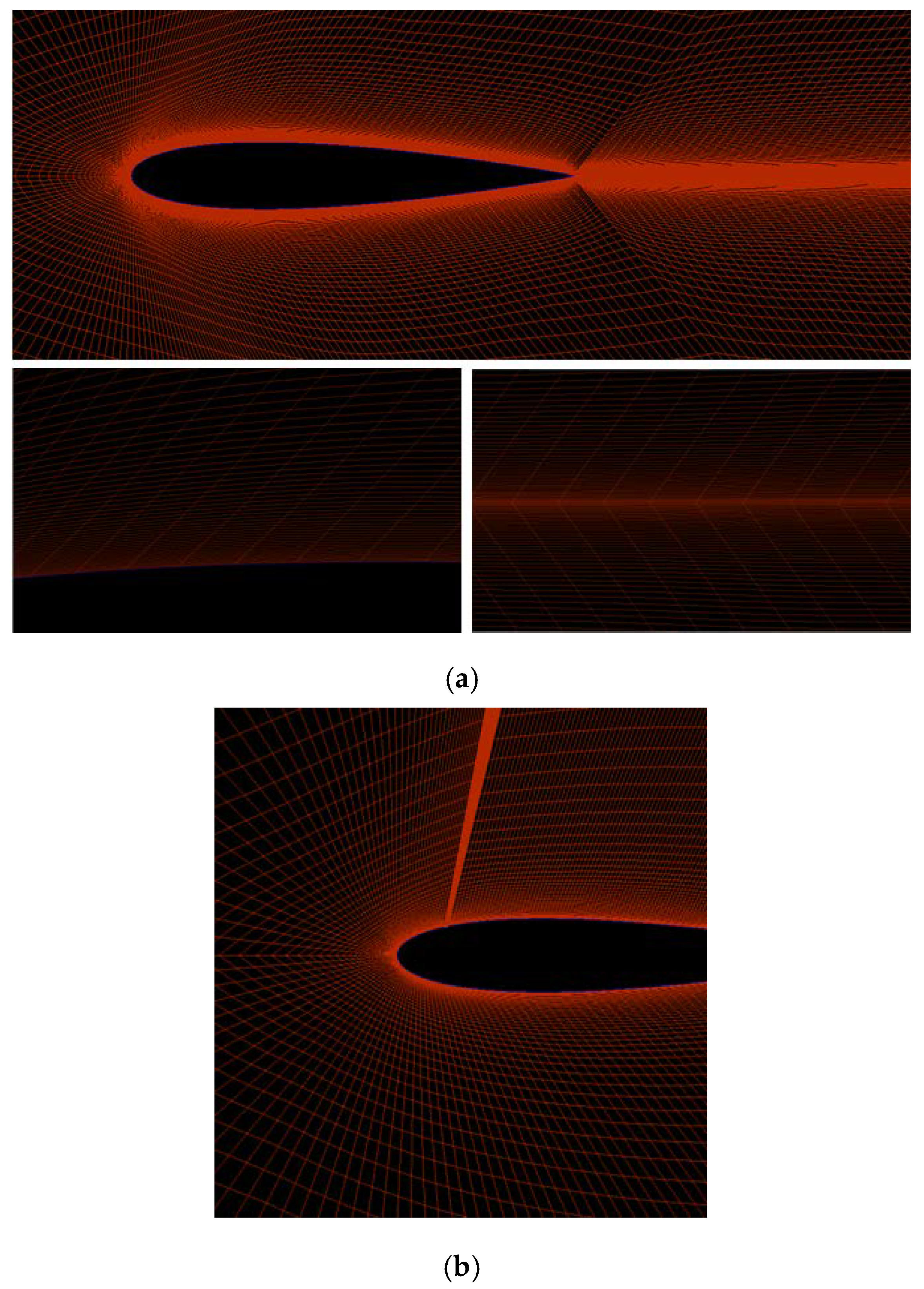
Figure 4.
Airfoil average lift coefficient as a function of angle of attack at chord Re = 106 (No-control case).
Figure 4.
Airfoil average lift coefficient as a function of angle of attack at chord Re = 106 (No-control case).

Figure 5.
Comparison of airfoil average drag coefficient against the angle of attack at chord Re = 106 (No-control case) with the experimental data and earlier numerical results.
Figure 5.
Comparison of airfoil average drag coefficient against the angle of attack at chord Re = 106 (No-control case) with the experimental data and earlier numerical results.

Figure 6.
The output static pressure signal as obtained from numerical simulations and used in the NARMAX construction.
Figure 6.
The output static pressure signal as obtained from numerical simulations and used in the NARMAX construction.

Figure 7.
(a) Variation of AIC and BIC with the NARMAX total number of parameters. (b) Variation of NSE efficiency with the NARMAX total number of parameters.
Figure 7.
(a) Variation of AIC and BIC with the NARMAX total number of parameters. (b) Variation of NSE efficiency with the NARMAX total number of parameters.

Figure 8.
(a) Time variations of the observed and predicted pressure signals at 250Hz. (b) Time variation of the absolute difference between the observed and estimated pressure signals .
Figure 8.
(a) Time variations of the observed and predicted pressure signals at 250Hz. (b) Time variation of the absolute difference between the observed and estimated pressure signals .
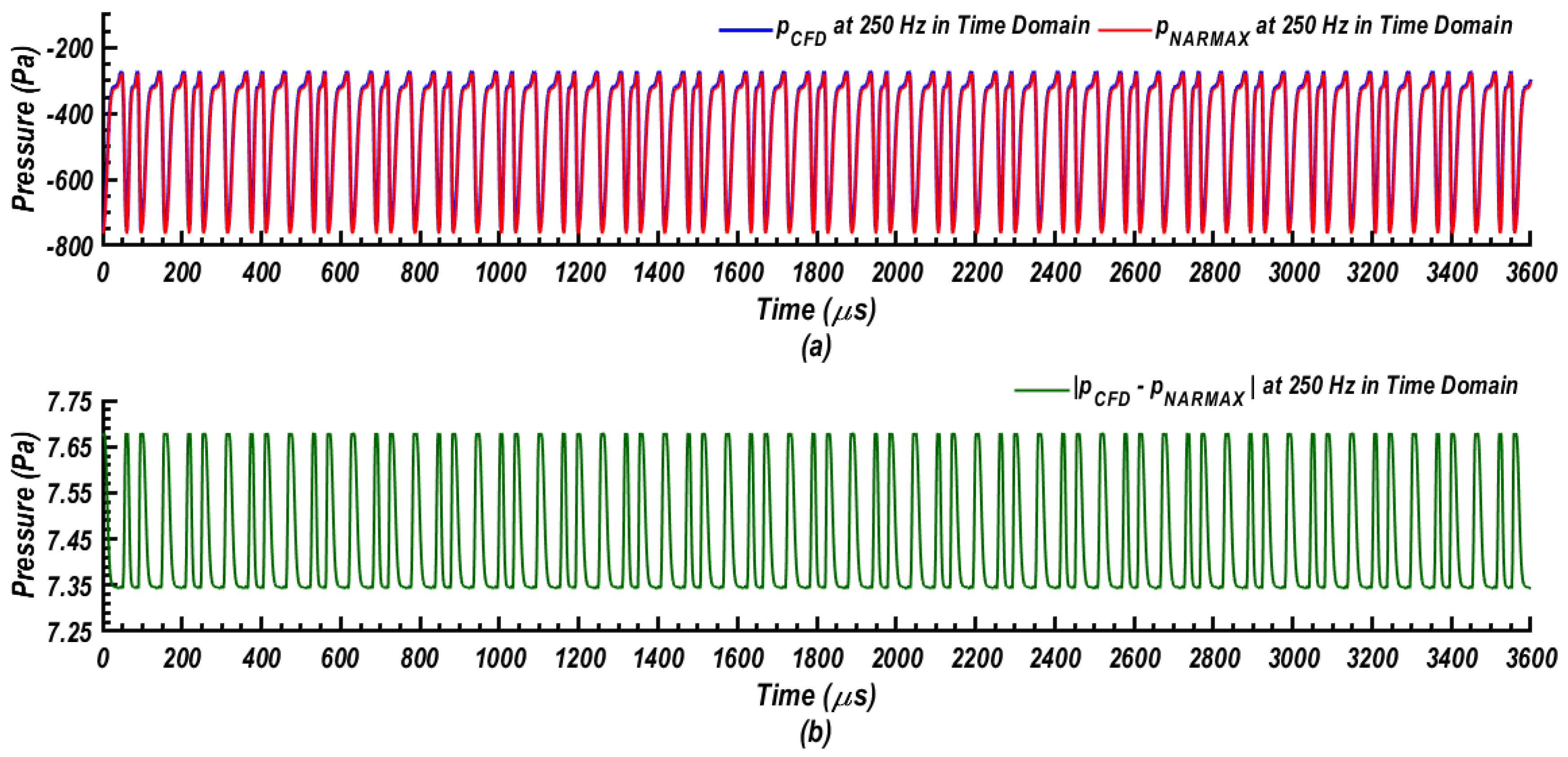
Figure 9.
Comparison of moving average of the pressure response as obtained from CFD calculations and NARMAX predictions for constant input.
Figure 9.
Comparison of moving average of the pressure response as obtained from CFD calculations and NARMAX predictions for constant input.
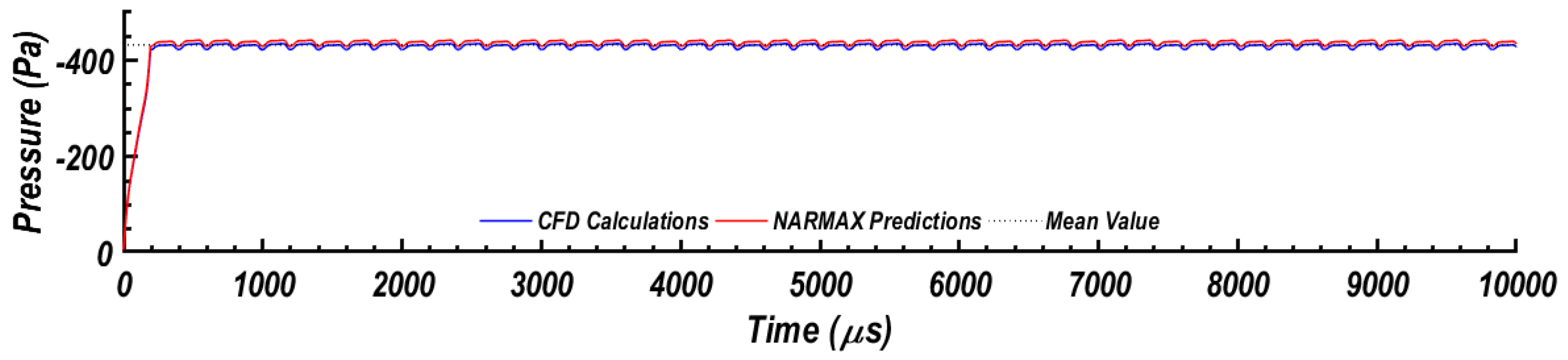
Figure 10.
Comparison of the power spectra of pressure signals. (a) Baseline flow (uncontrolled) and controlled flow with jet actuation at the frequency of 250 Hz. (b) CFD pressure signal and NARMAX estimated pressure signals with the jet driving frequency at 250Hz.
Figure 10.
Comparison of the power spectra of pressure signals. (a) Baseline flow (uncontrolled) and controlled flow with jet actuation at the frequency of 250 Hz. (b) CFD pressure signal and NARMAX estimated pressure signals with the jet driving frequency at 250Hz.

Figure 11.
Comparison between NARMAX model and CFD results for the mean pressure and SJA frequency at AoA = 16°
Figure 11.
Comparison between NARMAX model and CFD results for the mean pressure and SJA frequency at AoA = 16°
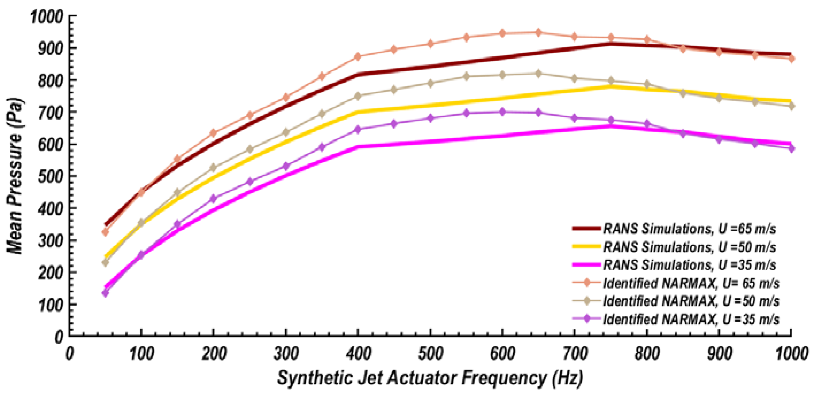
Figure 12.
Schematic diagram for the flow separation control.

Figure 13.
Schematic of an open-loop control system.
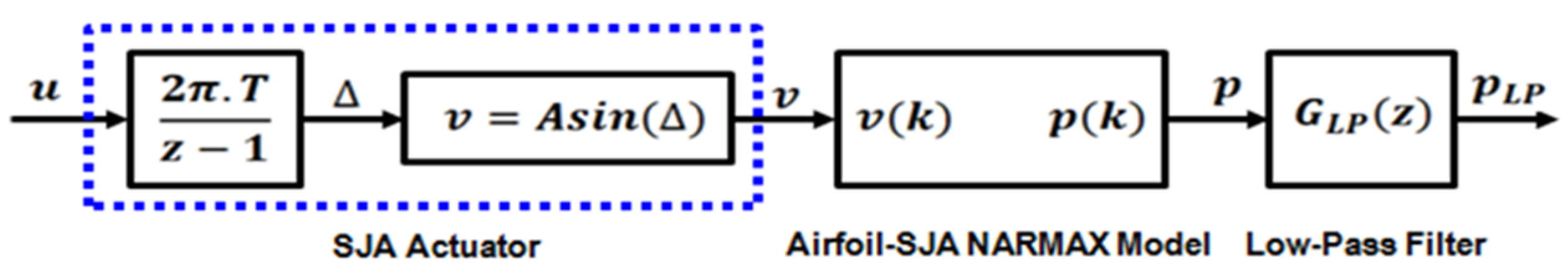
Figure 14.
Open-loop responses for the step inputs at 375 Hz, 775 Hz, and 1050 Hz. Time variations of (a) the synthetic jet frequency (), (b) synthetic jet velocity, , (c) static pressure signals as a result of synthetic jet actuation, and (d) filtered pressure signals from the low-pressure filter, .

Figure 15.
Simulink diagram for PI feedback control.

Figure 16.
Comparison of the power spectra of the predicted output pressure signals for the baseline and controlled flows with the synthetic jet actuation at 250 Hz and 629 Hz. (a) Higher than 108 power order and (b) in the range (106–107).
Figure 16.
Comparison of the power spectra of the predicted output pressure signals for the baseline and controlled flows with the synthetic jet actuation at 250 Hz and 629 Hz. (a) Higher than 108 power order and (b) in the range (106–107).

Figure 17.
A set of frequency responses of the linearized plant. (a) Magnitude in decibel versus frequency in Hz. (b) Phase in deg versus frequency in Hz.
Figure 17.
A set of frequency responses of the linearized plant. (a) Magnitude in decibel versus frequency in Hz. (b) Phase in deg versus frequency in Hz.
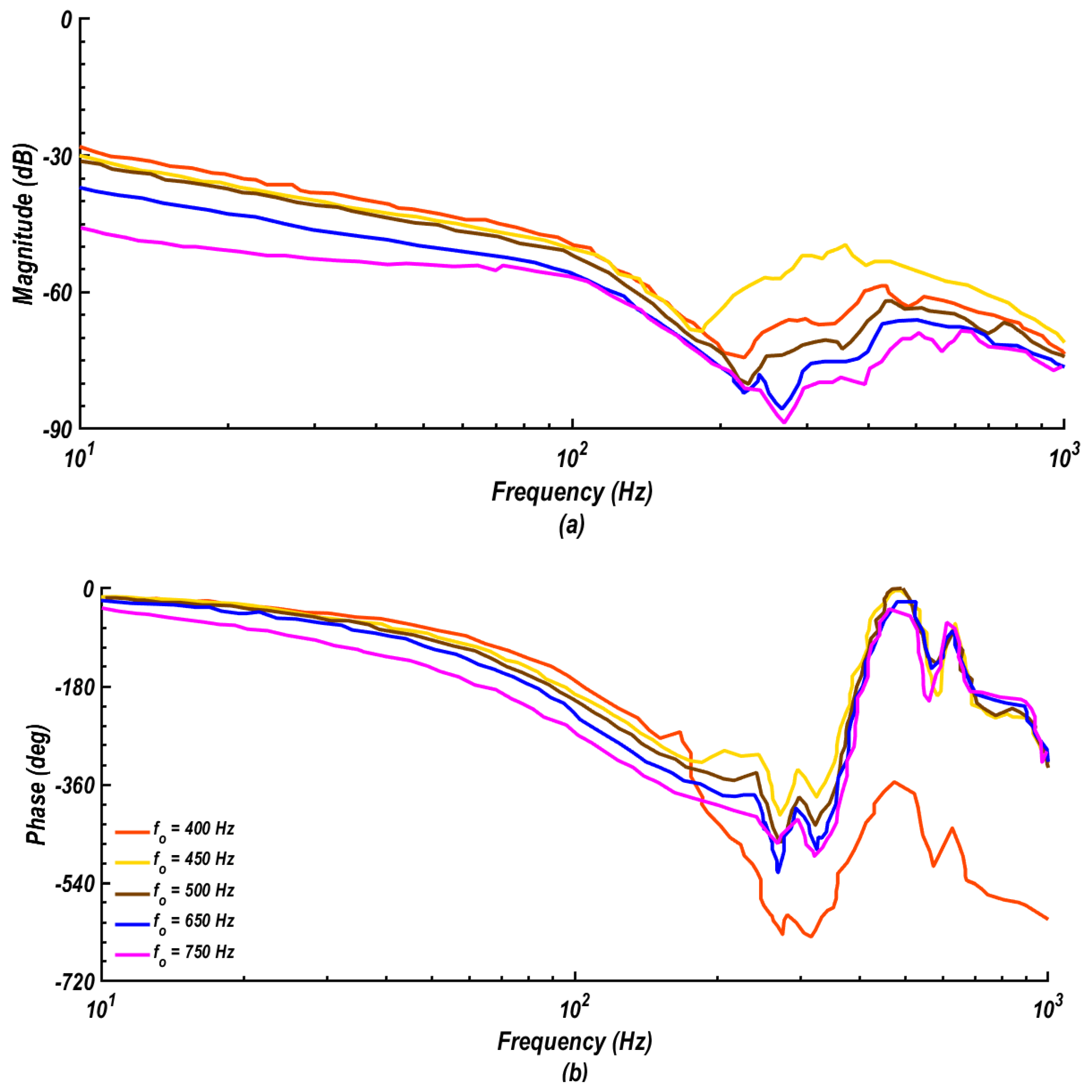
Figure 18.
A set of frequency responses of the open-loop transfer function of the controller-plant system, GpGc. (a) Magnitude in decibel versus frequency in Hz. (b) Phase in deg versus frequency in Hz.
Figure 18.
A set of frequency responses of the open-loop transfer function of the controller-plant system, GpGc. (a) Magnitude in decibel versus frequency in Hz. (b) Phase in deg versus frequency in Hz.
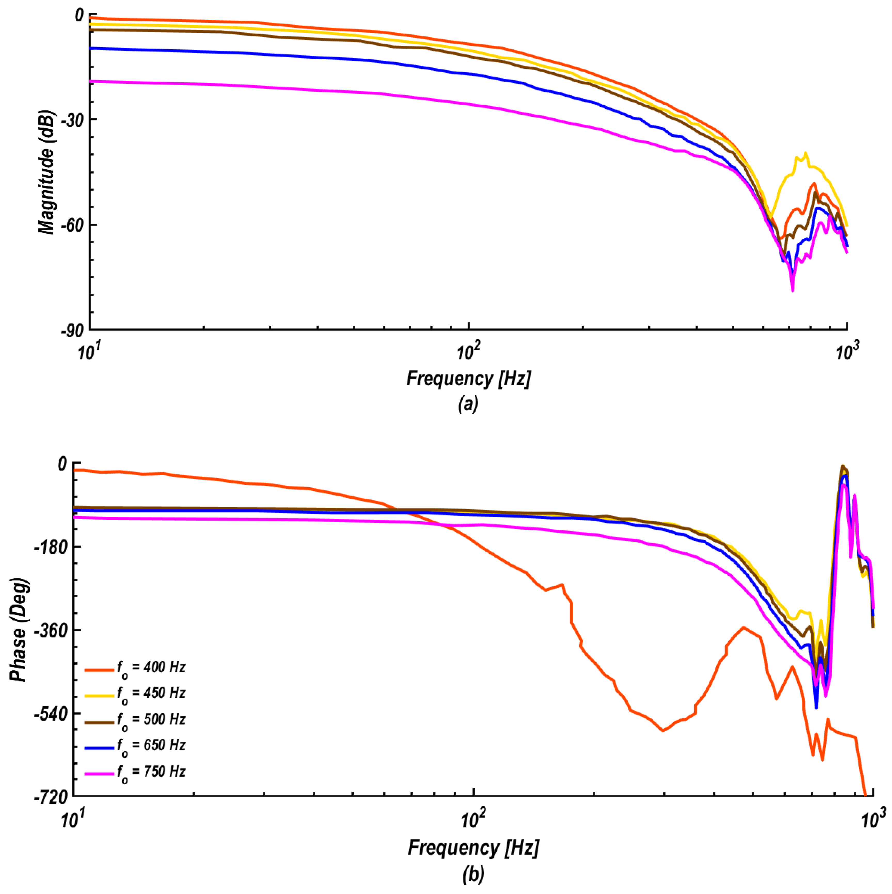
Figure 19.
System responses to step changes in the command signal for a proportional controller at various gain settings. (a) KP =1.636, (b) KP = 2.455, (c) KP = 3.273, (d) KP = 4.427, (e) KP = 5.581, and (f) KP = 6.735.
Figure 19.
System responses to step changes in the command signal for a proportional controller at various gain settings. (a) KP =1.636, (b) KP = 2.455, (c) KP = 3.273, (d) KP = 4.427, (e) KP = 5.581, and (f) KP = 6.735.

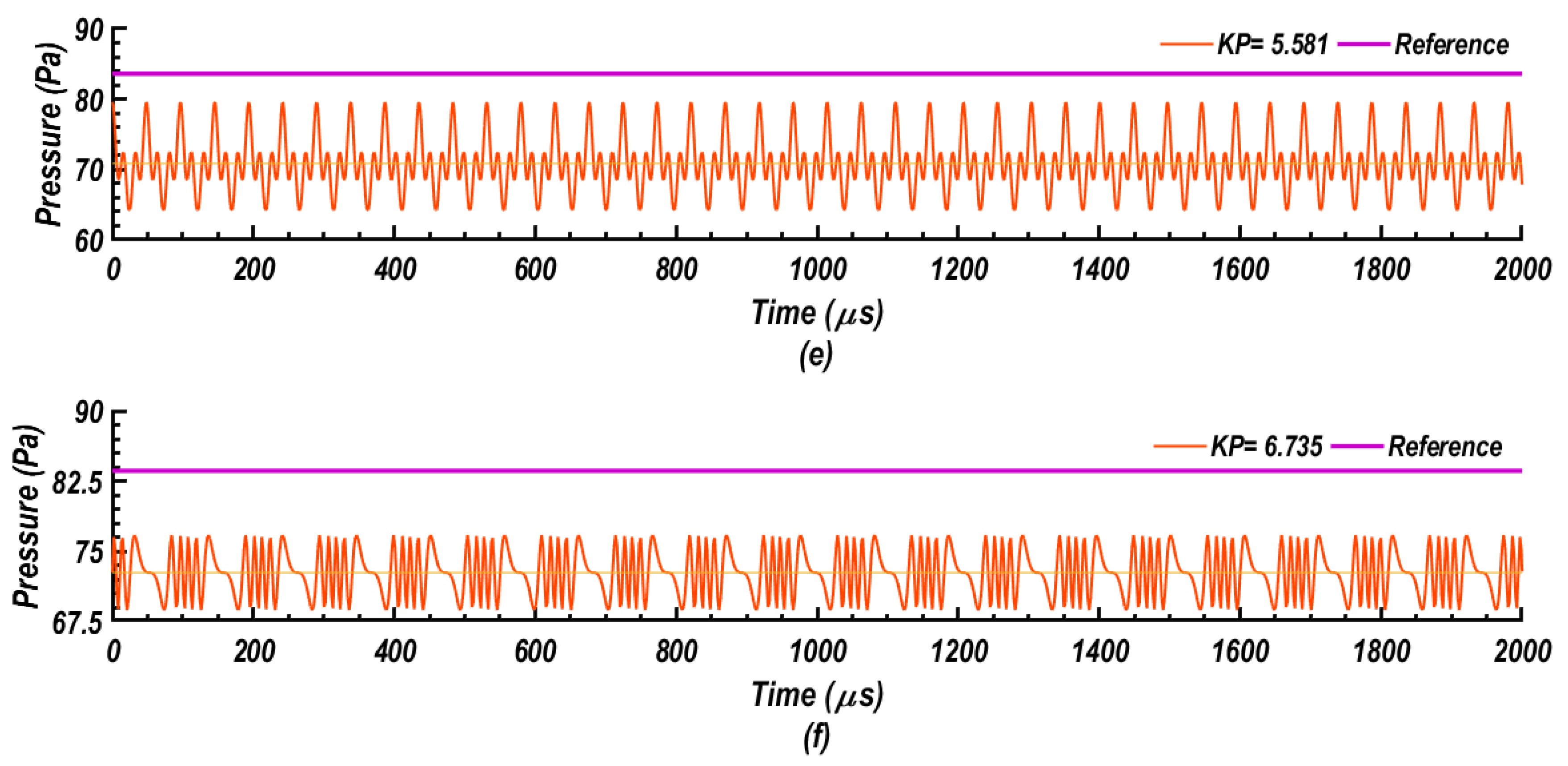
Figure 20.
Closed-loop step responses for PI controller for cases with (a) KP = 3.27 & various values of KI [0–0.330], and (b) KI = 0.083 and various values of KP [0–13.080].
Figure 20.
Closed-loop step responses for PI controller for cases with (a) KP = 3.27 & various values of KI [0–0.330], and (b) KI = 0.083 and various values of KP [0–13.080].

Figure 21.
Closed-loop responses using a PI controller with KP = 3.27 and KI = 0.083. (a) Time response of saturated SJA frequency, to step input (200 required by integral efforts to compensate feedback errors.) (b) Time response of pressure signal at 30% chord location to step input of 20 Pa. (200 required by integral efforts to compensate feedback errors.) and (c) Time response of pressure error signal to step input of 20 Pa. (Error signal reduces rapidly).

Figure 22.
Bode diagrams of the system. (a) Magnitude and phase plots of the PI Controller with KP = 3.27 and KI = 0.083. (b) Magnitude plot of the open-loop transfer function of the controller-plant system, GpGc, and (c) Phase plot of the open-loop transfer function of the controller-plant system, GpGc.
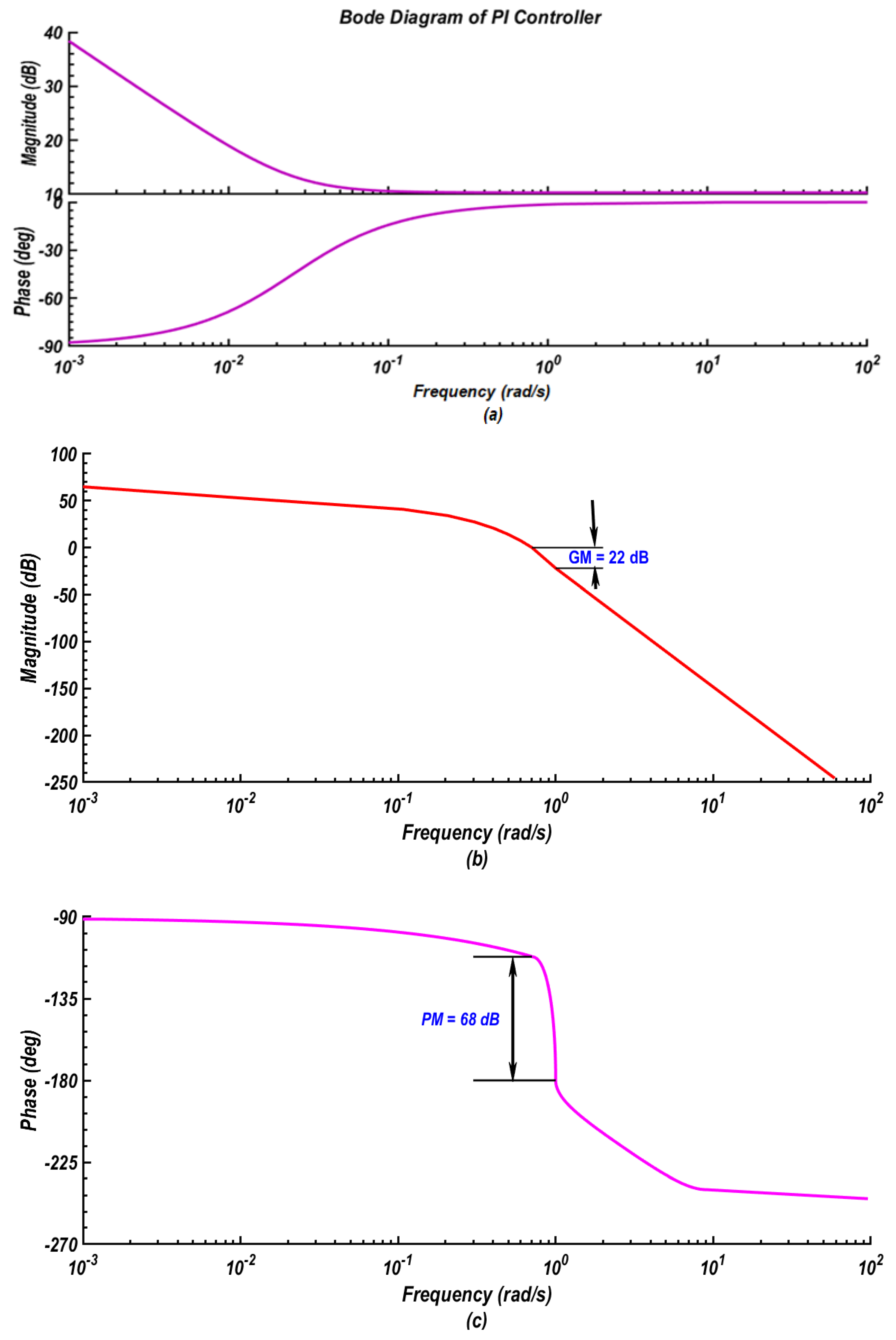
Figure 23.
Step responses of the PI controller with KP = 3.27 and KI = 0.083 for reference tracking and disturbance rejection. (a) Open-loop step response of PI controller. (b) Closed-loop step response of PI controller. (c) Closed-loop step response in case of input disturbance (). (d) Closed-loop step response in case of output disturbance ( ).


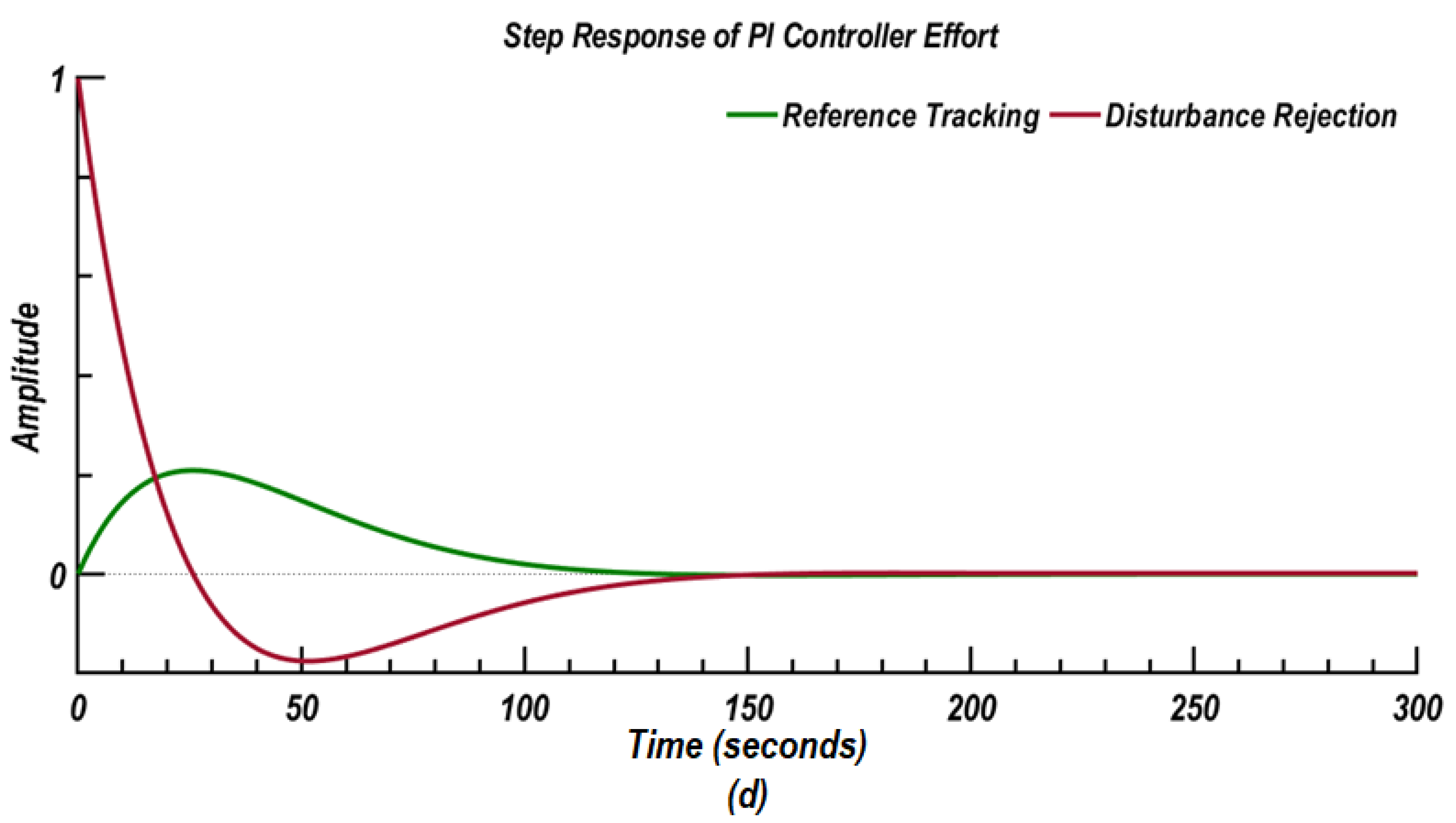
Figure 24.
Comparison of chord-wise average pressure coefficient curves along the sides of the airfoil at AoA = 16° for the control-off case and control-on cases.
Figure 24.
Comparison of chord-wise average pressure coefficient curves along the sides of the airfoil at AoA = 16° for the control-off case and control-on cases.
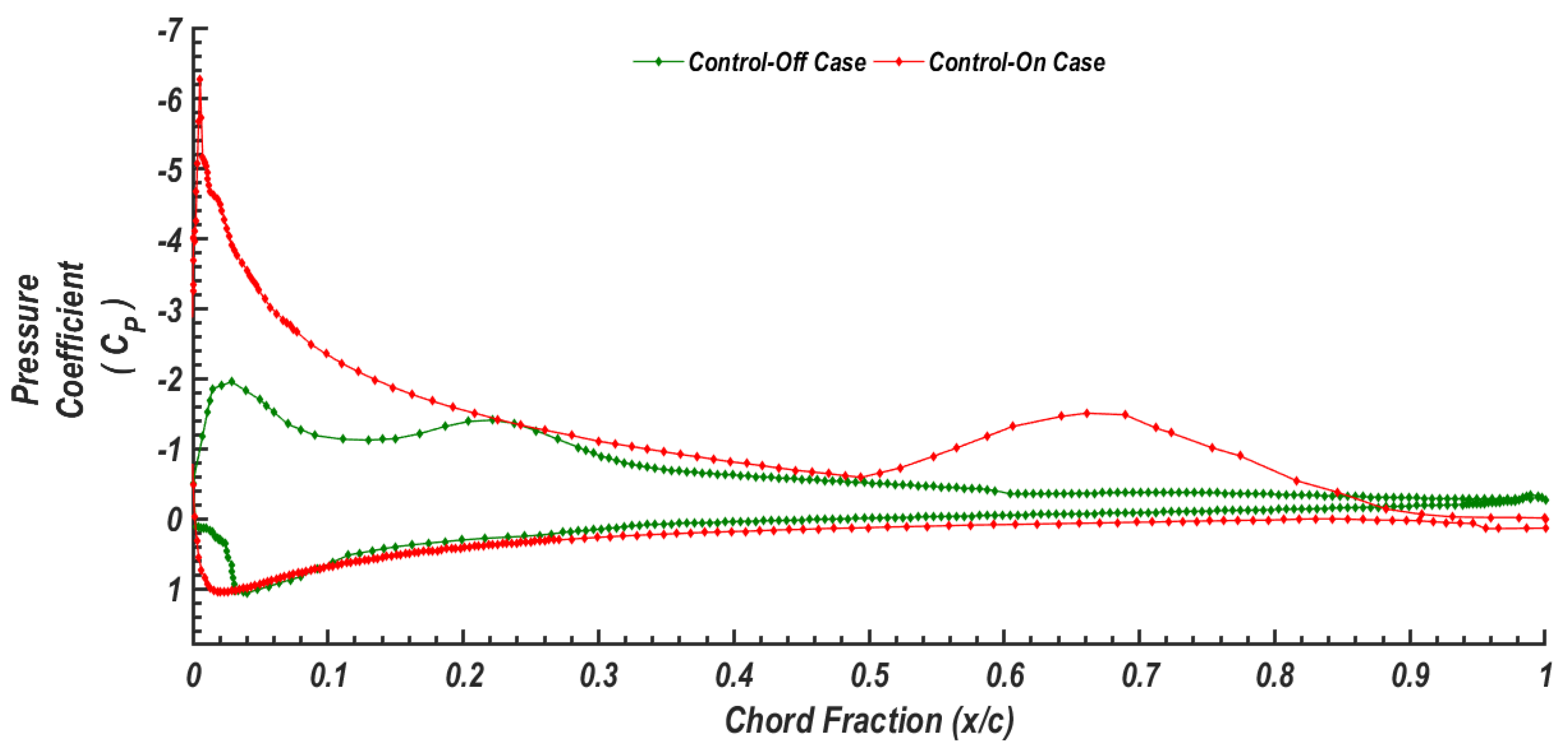
Figure 25.
Contours of the x-velocity component around the NACA 0015 airfoil at AoA = 16° for (a) control-off and (b) control-on case.
Figure 25.
Contours of the x-velocity component around the NACA 0015 airfoil at AoA = 16° for (a) control-off and (b) control-on case.
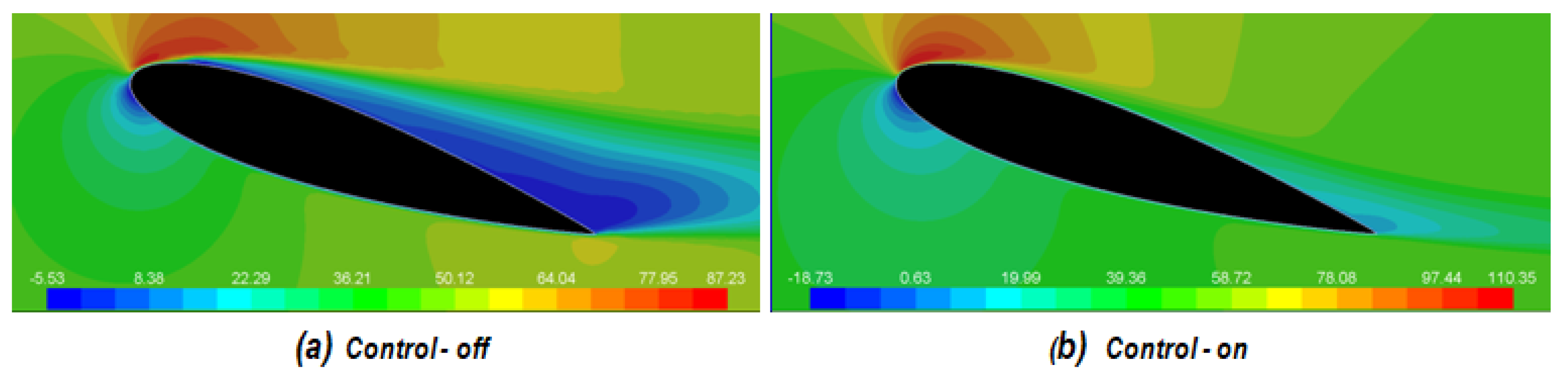
Figure 26.
Contours of turbulence kinetic energy around the NACA 0015 airfoil at AoA = 16° for (a) control-off and (b) control-on case.
Figure 26.
Contours of turbulence kinetic energy around the NACA 0015 airfoil at AoA = 16° for (a) control-off and (b) control-on case.
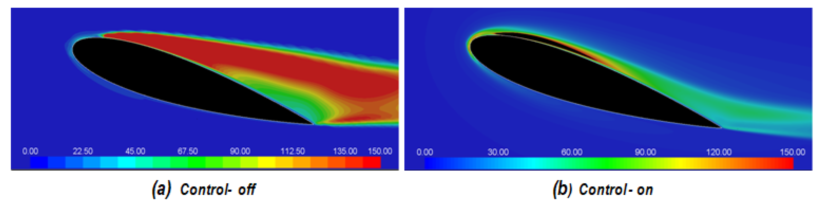
Figure 27.
Airfoil lift coefficient as a function of angle of attack at chord Re = 106 for control-off and control-on cases. Comparison with the earlier numerical results and experimental data.
Figure 27.
Airfoil lift coefficient as a function of angle of attack at chord Re = 106 for control-off and control-on cases. Comparison with the earlier numerical results and experimental data.
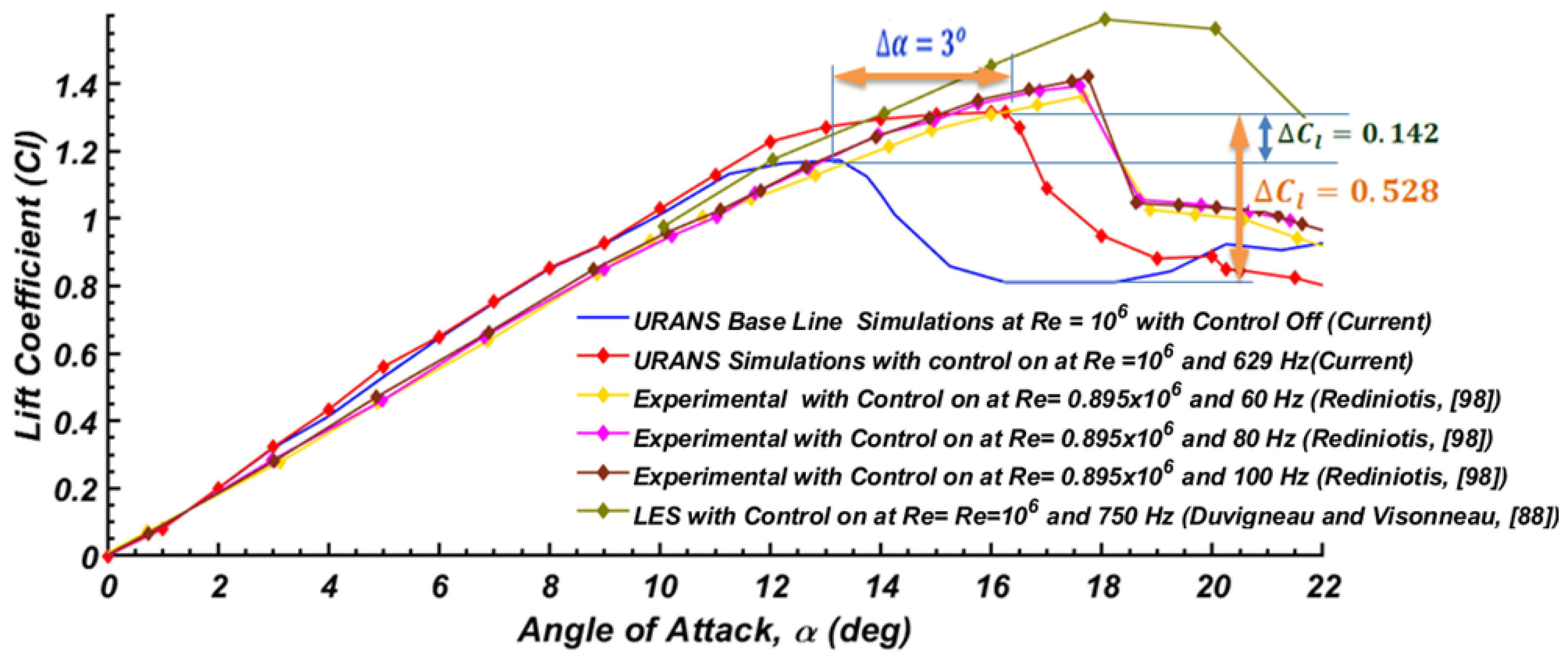
Figure 28.
Airfoil drag coefficient as a function of angle of attack at chord Re = 1 Million for control-off and control-on cases. Published numerical results and experimental data are also shown for comparison.
Figure 28.
Airfoil drag coefficient as a function of angle of attack at chord Re = 1 Million for control-off and control-on cases. Published numerical results and experimental data are also shown for comparison.
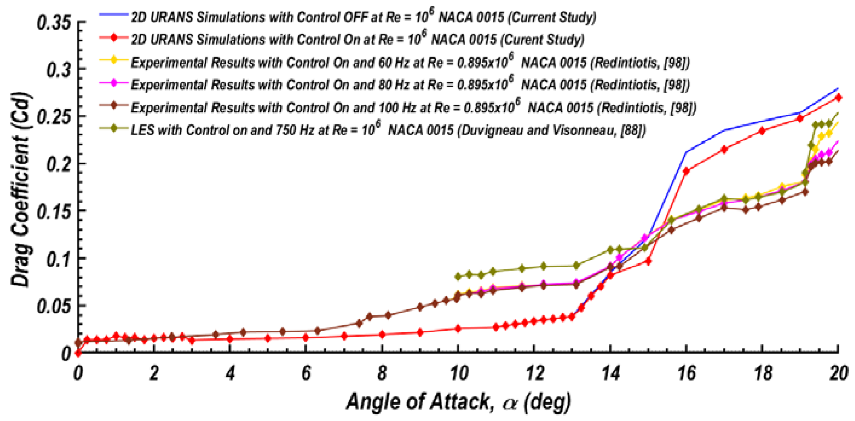
Figure 29.
Airfoil drag coefficient as a function of angle of attack at chord Re = 1 Million for control-off and control-on cases. Published numerical results and experimental data are also shown for comparison.
Figure 29.
Airfoil drag coefficient as a function of angle of attack at chord Re = 1 Million for control-off and control-on cases. Published numerical results and experimental data are also shown for comparison.

© 2020 by the authors. Licensee MDPI, Basel, Switzerland. This article is an open access article distributed under the terms and conditions of the Creative Commons Attribution (CC BY) license (http://creativecommons.org/licenses/by/4.0/).
Share and Cite
MDPI and ACS Style
Obeid, S.; Ahmadi, G.; Jha, R. NARMAX Identification Based Closed-Loop Control of Flow Separation over NACA 0015 Airfoil. Fluids 2020, 5, 100. https://doi.org/10.3390/fluids5030100
AMA Style
Obeid S, Ahmadi G, Jha R. NARMAX Identification Based Closed-Loop Control of Flow Separation over NACA 0015 Airfoil. Fluids. 2020; 5(3):100. https://doi.org/10.3390/fluids5030100
Chicago/Turabian StyleObeid, Sohaib, Goodarz Ahmadi, and Ratneshwar Jha. 2020. "NARMAX Identification Based Closed-Loop Control of Flow Separation over NACA 0015 Airfoil" Fluids 5, no. 3: 100. https://doi.org/10.3390/fluids5030100