Article

Breaking the Kolmogorov Barrier in Model Reduction of Fluid Flows

School of Mechanical and Aerospace Engineering, Oklahoma State University, Stillwater, OK 74078, USA
*
Author to whom correspondence should be addressed.
Fluids 2020, 5(1), 26; https://doi.org/10.3390/fluids5010026
Submission received: 15 January 2020 / Revised: 13 February 2020 / Accepted: 14 February 2020 / Published: 18 February 2020
(This article belongs to the Special Issue Recent Numerical Advances in Fluid Mechanics)

Abstract

:
Turbulence modeling has been always a challenge, given the degree of underlying spatial and temporal complexity. In this paper, we propose the use of a partitioned reduced order modeling (ROM) approach for efficient and effective approximation of turbulent flows. A piecewise linear subspace is tailored to capture the fine flow details in addition to the larger scales. We test the partitioned ROM for a decaying two-dimensional (2D) turbulent flow, known as 2D Kraichnan turbulence. The flow is initiated using an array of random vortices, corresponding to an arbitrary energy spectrum. We show that partitioning produces more accurate and stable results than standard ROM based on a global application of modal decomposition techniques. We also demonstrate the predictive capability of partitioned ROM through an energy spectrum analysis, where the recovered energy spectrum significantly converges to the full order model’s statistics with increased partitioning. Although the proposed approach incurs increased memory requirements to store the local basis functions for each partition, we emphasize that it permits the construction of more compact ROMs (i.e., of smaller dimension) with comparable accuracy, which in turn significantly reduces the online computational burden. Therefore, we consider that partitioning acts as a converter which reduces the cost of online deployment at the expense of offline and memory costs. Finally, we investigate the application of closure modeling to account for the effects of modal truncation on ROM dynamics. We illustrate that closure techniques can help to stabilize the results in the inertial range, but over-stabilization might take place in the dissipative range.

1. Introduction

Reduced order modeling (ROM) has been a hot topic in response to the increasing complexity of engineering systems and the requirement of near real-time and multi-query responses along with the limited advancement in computational resources [1,2,3,4,5]. This is vital for informed decision-making in the context of digital twins [6,7,8,9,10,11,12,13,14], model-based control [15,16,17,18,19,20,21,22], data assimilation [23,24,25,26,27,28,29,30,31,32,33], parameter estimation [34,35,36,37], and uncertainty quantification [38,39,40,41,42,43,44]. In fluid systems, this has been feasible thanks to the existence of a few underlying structures (e.g., vortices) that dominate the flow dynamics as well as the tremendous availability of data, which enables us to identify those structures (also called modes or basis functions) in a data-driven fashion [45,46,47,48,49,50,51,52,53,54,55,56,57]. However, most of the ROM developments have been applied mainly on prototypical flow problems. In particular, there is a limited number of investigations regarding ROMs in turbulent flows (e.g., see [58,59,60,61,62,63,64]). This is basically due to the excessive complexity of turbulent flows and existence of so many scales that interact with each other and control the mass, momentum, and energy transfer.
Challenges in the development of ROM for turbulent flows are also related to the Kolmogorov n-width for these systems. The Kolmogorov n-width is a concept from approximation theory that determines the linear reducibility of a system [65,66]. Mathematically, it is defined as [66,67,68]
d n ( M ) : = inf S n sup q M q Π S n q ,
where S n is a linear n-dimensional subspace, M is the solution manifold, and Π S n is the orthogonal projector onto S n . In other words, d n ( M ) quantifies the maximum possible error that might arise from the projection of solution manifold onto the best-possible n-dimensional linear subspace. When the decay of d n ( M ) with increasing n is fast, this means that the energy cascade and modal hierarchy allow the reduction of the system and the solution trajectory can be adequately approximated to evolve on a reduced linear subspace. However, for systems with strong nonlinearity, like turbulent flows, the intense interactions between different modes reduce the decay rate of the Kolmogorov n-width. Consequently, the linear reducibility is hindered. In ROM context, this is denoted as the “Kolmogorov barrier” because it necessitates involving more modes in ROM to guarantee sufficient approximation of the underlying dynamics. In short, turbulent flows are generally characterized by a slow decay of the Kolmogorov n-width, which raises the Kolmogorov barrier and the present work aims at addressing this issue.
In particular, we propose the use of a time domain partitioning approach, called principal interval decomposition (PID) [69,70,71,72,73] to break the Kolmogorov barrier of turbulent flows. PID has been investigated in previous studies and has been proven to be more accurate than standard ROMs based on the global basis construction (see [71,73] for example). Here, we aim at addressing a more complicated and involved flow problem characterizing two-dimensional turbulence. This allows us to investigate the effect of PID to capture the scales responsible for energy transfer and dissipation through an energy spectrum analysis. In addition, we relate the notion of the Kolmogorov barrier to the well-defined concept of relative information content in ROM context. Although turbulence is, by nature, three-dimensional, we investigate it in a simplified two-dimensional (2D) setting. It was shown that many aspects of idealized 2D turbulence are relevant for physical systems like geostrophic turbulence [74] and large-scale motions in the atmosphere and oceans [75,76]. The study of 2D turbulence idealizes geophysical phenomena and provides a starting point for their modeling. Specifically, we study ROM application on 2D Kraichnan turbulence. Moreover, we present a spectral study of the energy spectrum to emphasize the efficiency of PID approach for ROM in turbulence. Finally, we investigate the possibility of applying closure models for ROM stabilization. As a standard ROM technique, we employ proper orthogonal decomposition (POD) [46] for basis construction and Galerkin projection for dynamics approximation [58,77].
Fluid flow systems often include some sort of nonlinear interactions (e.g., corresponding to the convective effects). This implies that different modes (including the truncated ones) experience strong dynamical interactions between each others. Therefore, many modes need to be included for certain flows (especially for complex geometries and/or high Reynolds numbers). For example, Zhang and Stevens [78] stated that 2000 modes are necessary to capture 80 % of the total energy in a neutral atmospheric boundary layer (ABL) process, while Shah and Bou-Zeid [79] found that about 500 POD modes are required to capture the same amount of energy by using a two-dimensional snapshot POD. Nonetheless, the computational cost of a Galerkin ROM usually scales with R 3 in case of quadratic nonlinearity, where R is the number of retained/resolved modes. This necessitates the use of only a few modes for feasible ROM computations, especially for real-time control applications or multiple-query estimations. Other than the accuracy loss that would be incurred due to modal truncation, instabilities can easily occur. For instance, Östh et al. [80] showed a case for a flow around Ahmed body where the solution of a POD Galerkin model with 100 (or less) modes converges to infinity. Instabilities in standard ROMs have been attributed mainly to the truncation of higher modes, but Grimberg et al. [81] recently demonstrated that these instabilities are largely due to the standard Galerkin projection where the left and right set of basis functions match. To mitigate the instabilities encountered in Galerkin projection-based ROMs, Carlberg et al. [82] showed that least-squares Petrov–Galerkin can indeed build more accurate ROMs while Galerkin ROM becomes unstable for long time intervals. Alternatively, closure and stabilization models represent a feasible choice in the accuracy/stability-cost trade-off for Galerkin ROMs. Closure models have been popular in turbulence community, and found their way into ROM for fluid flows as well. Therefore, we also investigate the effect of a linear mode dependent eddy viscosity type closure model to stabilize the solution of ROM in case of 2D Kraichnan turbulence.

2. Two-Dimensional Kraichnan Turbulence

The two-dimensional (2D) turbulence cannot be realized in practice or experiments, but only in numerical simulations. Furthermore, 2D turbulence behaves differently from realistic 3D turbulence. In 3D turbulence, energy is transferred forward, from large scales to smaller scales, via vortex stretching. Conversely, in 2D turbulence, most of the forcing and dissipation energy will be transferred from smaller scales to larger scales and follows the Kraichnan–Batchelor–Leith (KBL) theory [83,84,85]. Despite the apparent simplicity in dealing with two spatial dimensions, 2D turbulence is very rich in its dynamics due to the inverse energy and forward enstrophy cascading mechanisms, which makes it a feasible testbed for a study of ROM in turbulence. Nonetheless, readers should be cautious while trying to extend the investigated framework into more realistic 3D turbulence cases.
The decaying homogeneous isotropic 2D Kraichnan turbulence follows the 2D Navier–Stokes equations, which can be written in vorticity-streamfunction formulation as below,
ω t + J ( ω , ψ ) = 1 Re 2 ω ,
where ω is the vorticity and ψ is the streamfunction. Re is Reynolds number relating the inertial and viscous effects. J ( ω , ψ ) and 2 ω are the Jacobian and Laplacian operators, respectively, which can be defined as
J ( ω , ψ ) = ω x ψ y ω y ψ x ,
2 ω = 2 ω x 2 + 2 ω y 2 .
The vorticity-streamfunction formulation enforces the incompressibility condition, where the vorticity and streamfunction fields are related by the following Poisson equation,
2 ψ = ω .
According to the KBL theory for 2D turbulence, the inertial range in the energy spectrum is proportional to k 3 in the inviscid limit. In our numerical experiments, the initial energy spectrum in Fourier space is given by
E ( k ) = 4 k 4 3 π k p 5 exp k k p 2 ,
where k = k x 2 + k y 2 and k p is the wavenumber at which the maximum value of initial energy spectrum occurs. During the time evolution process, due to the nonlinear interactions, this spectrum quickly approaches toward k 3 spectrum as we will show later when we present our results. The magnitude of the vorticity Fourier coefficients is related to the energy spectrum as
| ω ˜ ( k ) | = k π E ( k ) .
Then, the initial vorticity distribution (in Fourier space) is obtained by introducing a random phase. More details regarding derivation of the initial vorticity distribution from an assumed energy spectrum can be found in [86]. In the present study, we use a spatial computational domain of ( x , y ) [ 0 , 2 π ] × [ 0 , 2 π ] and a time domain of t [ 0 , 4 ] . Periodic boundary conditions are applied in both x- and y-directions. A spatial grid of 1024 2 and a timestep of Δ t = 0.001 are used. A fourth-order accurate Arakawa scheme [87] is used for spatial discretization and a third-order total variation diminishing Runge–Kutta scheme (TVD-RK3) [88] is adopted for temporal discretization.
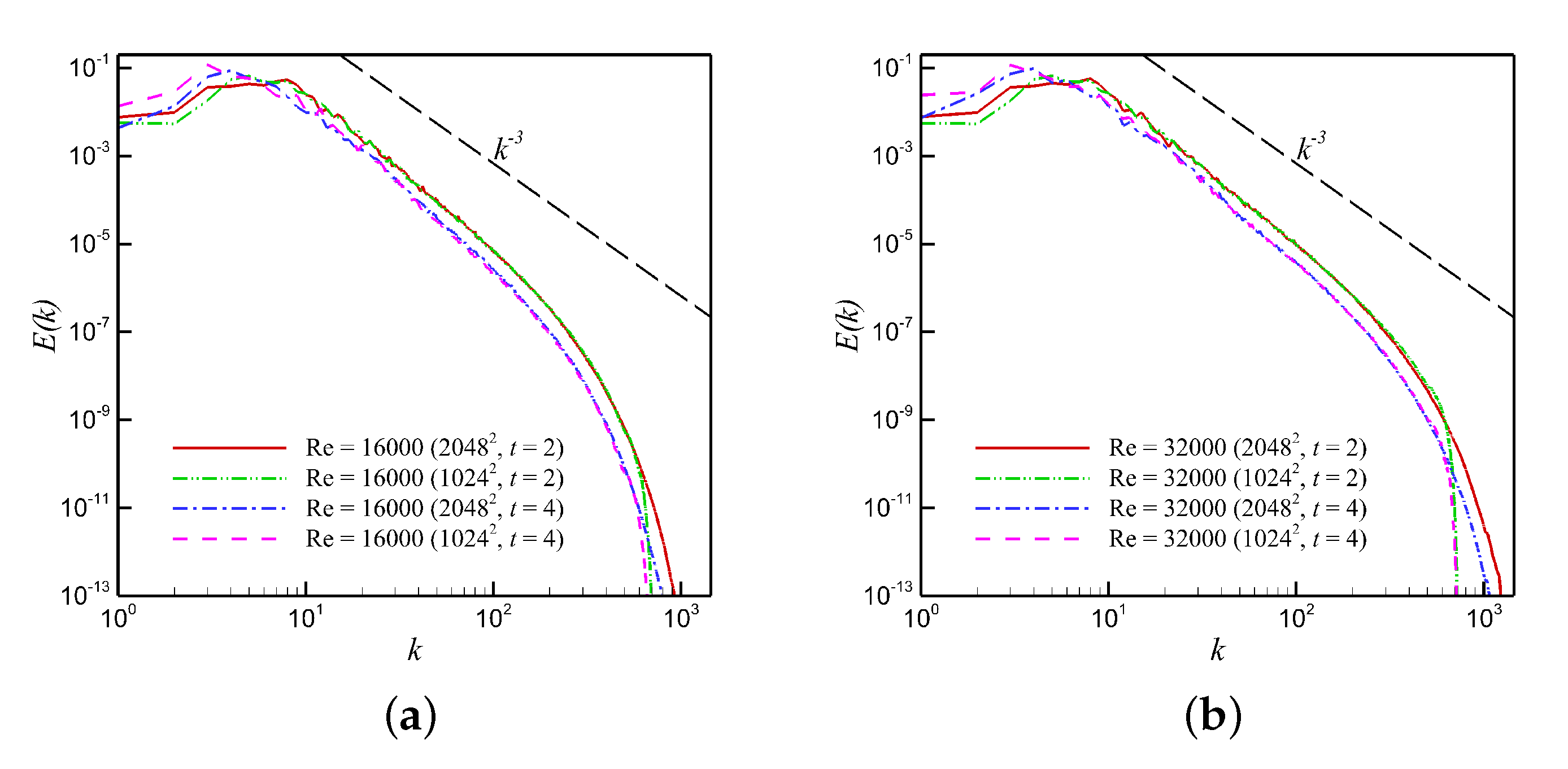
The energy spectrum for different values of Reynolds number is given in Figure 1 at t = 2 and t = 4 . We can observe that the energy spectrum in the inertial range flattens toward the classical k 3 scaling limit as Re increases, in agreement with the KBL theory for two-dimensional turbulence. It should be noted that the same initial vorticity distribution is enforced for all numerical experiments, by fixing the seed of the random numbers generator. In order to verify the validity of the used spatial resolution, Figure 2 shows the energy spectrum for Re = 16,000 (left) and Re = 32,000 (right) using two spatial resolutions (i.e., 1024 2 and 2048 2 ). A good match between the energy spectra corresponding to the two spatial resolutions can be seen, even for Re = 32,000. Nonetheless, we will consider Re = 16,000 with a spatial grid of 1024 2 for the rest of the present study. In addition, results obtained from solving Equation (2) using the aforementioned numerical schemes and resolution will be denoted as the full order model (FOM) results.

3. Reduced Order Modeling

In order to build a Galerkin projection-based reduced order model (ROM) of a physical system, the system’s state, u ( x , t ) , is assumed to live in a reduced trial subspace. Then, the high-dimensional operators are projected onto the same subspace, constraining the residual to be orthogonal to that subspace. Therefore, generating effective reduced subspaces that sufficiently contain the solution manifold is vital for the successful construction of Galerkin ROMs. One of the very early-developed and well-known approaches to build reduced subspaces is Fourier analysis. However, it assumes universal basis functions (or modes) which have no specific relation to the system in hand, except for boundary conditions. More efficiently, snapshot-based model reduction techniques can tailor a reduced subspace that best fits the problem by extracting the underlying coherent structures that control the major dynamical evolution we are interested in. Among those snapshot-based techniques, proper orthogonal decomposition (POD) is the most popular and well-established approach extracting the modes which contribute the most to the total system’s energy [4,89]. The basic implementation of POD is presented in the following subsection.

3.1. Proper Orthogonal Decomposition

As mentioned before, proper orthogonal decomposition (POD) is a snapshot-based approach. Therefore, a collection of system’s realizations (called snapshots) are required in advance. Assuming that a number of snapshots ( N s ) of the 2D vorticity field, denoted as ω ( x , y , t n ) , are stored at consecutive times t n for n = 1 , 2 , , N s , the time-averaged field, called “base flow”, can be computed as
ω ¯ ( x , y ) = 1 N n = 1 N ω ( x , y , t n ) .
The mean-subtracted snapshots, also called anomaly or fluctuation fields, are then computed as the difference between the instantaneous fields and the mean field,
ω ( x , y , t n ) = ω ( x , y , t n ) ω ¯ ( x , y ) .
This mean-subtraction is common in ROM community, and it guarantees that ROM solution would satisfy the same boundary conditions as a full order model [90]. This anomaly field procedure is also interpreted as a mapping of snapshot data to its origin (i.e., centering), and will be used for constructing the POD basis functions. The POD approach basically relies on an eigenvalue decomposition of a snapshot correlation (or covariance) matrix. Since the number of snapshots ( O ( 10 2 ) ) is usually much less than the number of grid points ( O ( 10 6 ) ), we follow the method of snapshots [54] for efficient implementation of the POD algorithm.
An N s × N s temporal correlation data matrix A = [ a i j ] is computed from the inner product of temporal anomaly fields as
a i j = ω ( x , y , t i ) ; ω ( x , y , t j ) ,
where the angle-parenthesis denotes the inner product in Hilbert space defined as
ω ( x , y , t i ) ; ω ( x , y , t j ) = Ω ω ( x , y , t i ) ω ( x , y , t j ) d x d y ,
where Ω represent the physical (spatial) domain. Then, an eigenvalue decomposition of A is performed as
A V = V Λ ,
where Λ is a diagonal matrix whose entries are the eigenvalues λ k of A , and V is a matrix whose columns v k are the corresponding eigenvectors. A is a Gramian matrix, a property which can be utilized for efficient solution of the eigenvalue problem (e.g., using Jacobi transformations [91]). The eigenvalues λ k represent the amount of information contained in each mode; therefore, they should be arranged in a descending order (i.e., λ 1 λ 2 λ N ), for proper selection of the POD modes. The POD modes ϕ k are finally computed as
ϕ k ( x , y ) = 1 λ k n = 1 N v k n ω ( x , y , t n ) ,
where v k n is the n-th component of the eigenvector v k . It can be easily verified that the POD modes are orthonormal (i.e., ϕ i ; ϕ j = δ i j ), which simplifies the derivation of ROM.

3.2. Galerkin Projection

With the POD algorithm implemented, a set of POD basis functions are obtained { ϕ k ( x , y ) } k = 1 R , where R is the number of POD modes retained in ROM (i.e., the size of the reduced subspace). The solution is therefore approximated as a superposition of the contributions of these selected modes as follows:
ω ( x , y , t ) = ω ¯ ( x , y ) + k = 1 R α k ( t ) ϕ k ( x , y ) ,
where α k ( t ) are the so-called temporal modal coefficients. Since the vorticity and streamfunction are related by the kinematic relationship given by Equation (5), the basis functions ( θ k ( x , y ) ) and mean field ( ψ ¯ ( x , y ) ) corresponding to the streamfunction can be obtained from those of the vorticity as follows:
2 ψ ¯ ( x , y ) = ω ¯ ( x , y ) ,
2 θ k ( x , y ) = ϕ k ( x , y ) , k = 1 , 2 , , R ,
which might result in a set of basis functions for the streamfunction that are not necessarily orthonormal. Moreover, the reduced order approximation of streamfunction can share the same temporal coefficients α k ( t ) ,
ψ ( x , y , t ) = ψ ¯ ( x , y ) + k = 1 R α k ( t ) θ k ( x , y ) .
Those approximations are then substituted in Equation (2), as follows:
t ω ¯ ( x , y ) + k = 1 R α k ( t ) ϕ k ( x , y ) = J ω ¯ ( x , y ) + k = 1 R α k ( t ) ϕ k ( x , y ) , ψ ¯ ( x , y ) + k = 1 R α k ( t ) θ k ( x , y ) + 1 Re 2 ω ¯ ( x , y ) + k = 1 R α k ( t ) ϕ k ( x , y ) .
Then, we use the definition of Jacobian operator and expand the above expression as
t ω ¯ ( x , y ) + t k = 1 R α k ( t ) ϕ k ( x , y ) = J ω ¯ ( x , y ) , ψ ¯ ( x , y ) J k = 1 R α k ( t ) ϕ k ( x , y ) , k = 1 R α k ( t ) θ k ( x , y ) J ω ¯ ( x , y ) , k = 1 R α k ( t ) θ k ( x , y ) J k = 1 R α k ( t ) ϕ k ( x , y ) , ψ ¯ ( x , y ) + 1 Re 2 ω ¯ ( x , y ) + 1 Re 2 k = 1 R α k ( t ) ϕ k ( x , y ) .
Note that the first term t ω ¯ ( x , y ) is zero. In addition, the Jacobian and Laplacian operators are spatial functions; therefore, the following can be written (after change of indices)
t i = 1 R α i ( t ) ϕ i ( x , y ) = J ω ¯ ( x , y ) , ψ ¯ ( x , y ) i = 1 R j = 1 R α i ( t ) α j ( t ) J ϕ i ( x , y ) , θ j ( x , y ) i = 1 R α i ( t ) J ω ¯ ( x , y ) , θ i ( x , y ) i = 1 R α i ( t ) J ϕ i ( x , y ) , ψ ¯ ( x , y ) + 1 Re 2 ω ¯ ( x , y ) + i = 1 R α i ( t ) 1 Re 2 ϕ i ( x , y ) .
Then, we can collect the constant, linear, and nonlinear terms (in time) as follows:
t i = 1 R α i ( t ) ϕ i ( x , y ) = J ω ¯ ( x , y ) , ψ ¯ ( x , y ) + 1 Re 2 ω ¯ ( x , y ) + i = 1 R α i ( t ) J ω ¯ ( x , y ) , θ i ( x , y ) J ϕ i ( x , y ) , ψ ¯ ( x , y ) + 1 Re 2 ϕ i ( x , y ) i = 1 R j = 1 R α i ( t ) α j ( t ) J ϕ i ( x , y ) , θ j ( x , y ) .
Finally, an inner product with an arbitrary basis function ϕ k ( x , y ) is performed, where we make use of the orthonormality of the vorticity basis functions. Therefore, a reduced order model is obtained, which can be simply represented by the following set of ODEs for α k ( t ) ,
d α k d t = B k + i = 1 R L i , k α i + i = 1 R j = 1 R N i , j , k α i α j , k = 1 , 2 , , R ,
where the predetermined model coefficients can be computed by the following numerical integration (offline computing)
B k = J ( ω ¯ , ψ ¯ ) + 1 Re 2 ω ¯ ; ϕ k , L i , k = J ( ω ¯ , θ i ) J ( ϕ i , ψ ¯ ) + 1 Re 2 ϕ i ; ϕ k , N i , j , k = J ( ϕ i , θ j ) ; ϕ k .
To complete the dynamical system given by Equation (18), the initial conditions for α k ( t ) may be obtained by the following projection of the initial vorticity field onto the respective basis functions,
α k ( t 0 ) = ω ( x , y , t 0 ) ω ¯ ( x , y ) ; ϕ k ,
where ω ( x , y , t 0 ) is the vorticity field specified at initial time t 0 .
We note that the approach described here is called tensorial ROM, since the model predetermined terms (especially those corresponding to nonlinear terms) are computed in advance as tensors during an offline stage, while the online solution of Equation (18) scales with R 3 . Alternatively, the model terms can be calculated online while minimizing the cost of computing the nonlinear terms through approximating approaches like discrete empirical interpolation method (DEIM) [92,93], gappy POD [60,94], and missing point estimation (MPE) [95,96]. An overview of these techniques can be found in [97,98].

4. Partitioned ROM

A representative solution subspace is a key factor in the construction of ROMs of physical systems and POD has been successfully offering a systematic approach for building such a subspace. However, POD in principle depends on a global approximation of the snapshot data. This has several consequences, a few of which are mentioned here. First, local temporary excursions in state space which contain small amounts of energy can be overlooked by POD because their contribution to the total energy may be negligible. These excursions can, however, be of interest and have significant impact on the dynamical evolution (see [99], for example). Second, the global nature of POD approach can result in overall deformation of the obtained modes for systems with fast variations in state. As a result, the constructed POD modes are smoothed out and cannot capture any dominant structure at all. This in turn causes an energy distribution across a large number of modes; therefore, the truncated modes contain a significant amount of system’s energy, which causes inaccuracies and instabilities in the solution unless the size of the ROM is increased.
An alternative approach which preserves the optimality of POD, while giving care to the system’s local characteristics, is called principal interval decomposition (PID) [69,70,71,72,73]. In PID, the time domain is divided into a few partitions, each characterizing a specific stage in the system’s dynamics and evolution. Then, the same POD algorithm is applied within each partition to generate a set of basis functions that best fit the respective partition locally. In a sense, the PID approach can be viewed as decomposing the global POD subspace into a few of locally optimal subspaces. As a result, accurate partitioned ROMs with smaller sizes can be dedicated to each individual sub-interval. More details about the properties of PID can be found in [73]. This partitioning idea can also be performed in the physical domain, state space, or parameter space [64,100,101,102].
In brief, the time domain T = [ t 0 , t f ] is divided into a number P of non-overlapping partitions (every two consecutive partitions share only the interface). Adaptive partitioning and clustering techniques can be used to tailor partitions with arbitrary widths if no a priori information is available about the dynamics of the systems. However, for simplicity and clarity of presentation, we assume equidistant decomposition of the time domain. In other words, the total number of snapshots N s is divided into N s / P sets. After that, local mean fields ω ¯ ( l ) ( x , y ) and ψ ¯ ( l ) ( x , y ) are computed and the POD algorithm described in Section 3.1 is applied to each group of snapshots to generate local basis functions { ϕ k ( l ) ( x , y ) } k = 1 R and { θ k ( l ) ( x , y ) } k = 1 R for l = 1 , 2 , , P . Then, the Galerkin ROM equations are obtained for each interval as
d α k ( l ) d t = B k ( l ) + i = 1 R L i , k ( l ) α i ( l ) + i = 1 R j = 1 R N i , j , k ( l ) α i ( l ) α j ( l ) , k = 1 , 2 , , R , l = 1 , 2 , , P ,
where the predetermined model coefficients can be computed partition-wise by the following numerical integrations:
B k ( l ) = J ( ω ¯ ( l ) , ψ ¯ ( l ) ) + 1 Re 2 ω ¯ ( l ) ; ϕ k ( l ) , L i , k ( l ) = J ( ω ¯ ( l ) , θ i ( l ) ) J ( ϕ i ( l ) , ψ ¯ ( l ) ) + 1 Re 2 ϕ i ( l ) ; ϕ k ( l ) , N i , j , k ( l ) = J ( ϕ i ( l ) , θ j ( l ) ) ; ϕ k ( l ) ,
and the initial conditions for α k ( 1 ) ( t ) are obtained by the following projection:
α k ( 1 ) ( t 0 ) = ω ( x , y , t 0 ) ω ¯ ( 1 ) ( x , y ) ; ϕ k ( 1 ) .
It remains to enforce the interface constraints to enable solution transition from one partition to the next, if no access to the true field at the interface instant is available. We do so by imposing the following condition at the interface [103],
ω ( l ) ( x , y , t l ) ω ( l + 1 ) ( x , y , t l ) ; ϕ k ( l + 1 ) = 0 ,
where t l represents the time instant at the interface between the interval l and l + 1 . Here, ω ( l ) ( x , y , t l ) is the reconstructed vorticity field at the interface using the left interval (l), while ω ( l + 1 ) ( x , y , t l ) is reconstructed at the same instant, but using the right interval ( l + 1 ). Those can be rewritten as
ω ( l ) ( x , y , t l ) = ω ¯ ( l ) ( x , y ) + k = 1 R α k ( l ) ( t l ) ϕ k ( l ) ( x , y ) ,
ω ( l + 1 ) ( x , y , t l ) = ω ¯ ( l + 1 ) ( x , y ) + k = 1 R α k ( l + 1 ) ( t l ) ϕ k ( l + 1 ) ( x , y ) .
This reduces to performing the following computation at the interface to re-initiate our solver at the first timestep of the new time interval,
α k ( l + 1 ) ( t l ) = i = 1 R α i ( l ) ( t l ) ϕ i ( l ) ( x , y ) + ω ¯ ( l ) ( x , y ) ω ¯ ( l + 1 ) ( x , y ) ; ϕ k ( l + 1 ) ( x , y ) .

5. Results

As indicated in Section 2, the full order model is solved over a square domain with a side length of 2 π using a spatial grid of 1024 2 for t [ 0 , 4 ] with a timestep of 0.001 . These were shown to be sufficient resolutions to solve the problem at a Reynolds number of 16 , 000 . To build the reduced order subspace using the POD and PID algorithms, described in Section 3.1 and Section 4, 800 snapshots of vorticity field were collected (i.e., every five timesteps). It was also shown that the sampling rate has minor effect on POD-based modal decomposition, as long as the Nyquist–Shannon sampling criterion is met [104]. Another factor we consider in our choice of sampling rate is to have adequate number of snapshots in each sub-interval (after partitioning the time domain).
The partitioned ROM approach is used to solve Equation (21) using different numbers of partitions. In particular, we present the results for P { 1 , 4 , 8 } . Note that, for P = 1 , the approach reduces to the standard Galerkin-POD ROM with a single interval covering the whole time domain. In Figure 3, the energy spectrum at t = 4 is used to illustrate the effect of increasing the number of partitions on ROM accuracy and convergence to the FOM solution. This is shown for P = 1 (top), P = 4 (middle), and P = 8 (bottom), along with a compensated (for zooming-in) view of the energy spectrum at the inertial range on the right. We can easily observe that increasing the number of partitions improves the convergence of ROM energy spectrum to the true one for all values of R.
Although increasing the number of retained modes generally improves the ROM accuracy, this does not help a lot in the case with P = 1 . This is shown in Figure 3, where we still see a large deviation of ROM results in the inertial range even with 32 modes. This might be attributed to the smoothing-out of constructed basis functions in such a way that information is distributed across a large number of modes. Consequently, the effect of modal truncation on system’s dynamics is no more negligible. On the other hand, a partitioned ROM with P = 8 enables us to build accurate ROMs with relatively compact sizes (e.g., R = 16 ).
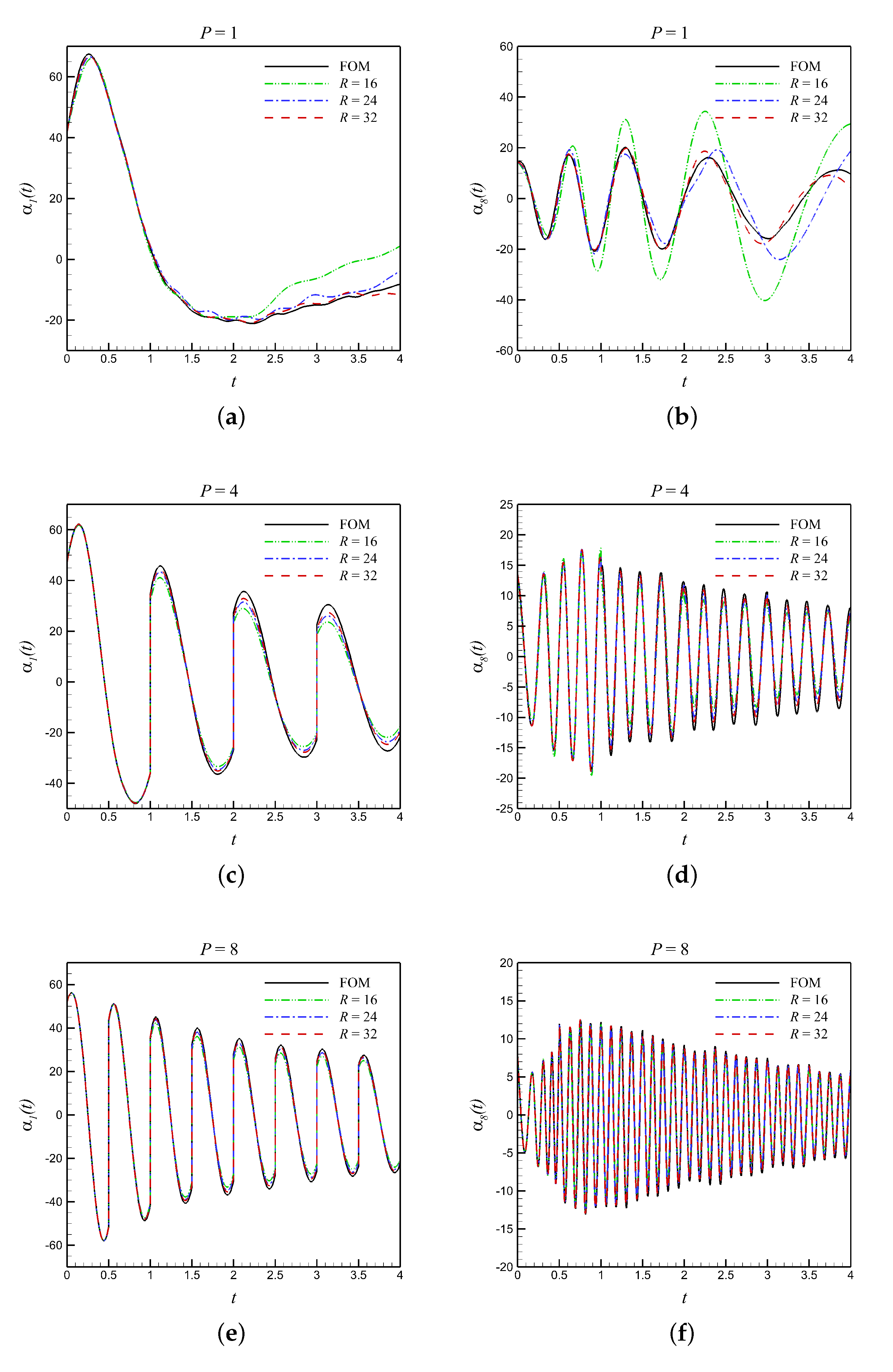
To provide more insights about the scales resolved with partitioned ROM, we plot the evolution of the temporal coefficients of the first and eighth modes in Figure 4. We can notice that a ROM with global POD modes (i.e., P = 1 ) can adequately capture the evolution of the first mode’s contribution (with increasing deviations toward the end of the time domain). On the other hand, a phase shift and amplification of the temporal evolution of the 8th modal coefficient are spotted after a small initial period. From a physical point of view, the first modes correspond to the large dominating scales, while the last ones correspond to the small (or fine) scales. This indicates that a global POD application provides ROMs that moderately capture the large scales, but can fail to capture the finer details. Moreover, we can deduce from Figure 4a that the dynamics at different time instants is different (where all the snapshots are projected onto the same set of basis functions). This justifies the use of paritioned ROM to tailor unique bases for each sub-interval. On the other hand, with partitioned ROMs (i.e., P = 4 and P = 8 ), the evolution of both α 1 and α 8 is tracked accurately, implying that the presented partitioning approach improves the ROM’s capabilities to represent the fine scales. Moreover, the accuracy of α 1 prediction is improved compared to P = 1 . Although the evolution of temporal coefficients in different sub-intervals looks similar, this is because the fields in each region are projected onto their respective bases. Therefore, once reconstructed, the dynamics in the full order space will be different. In addition, we can note the “jump” at the interfaces (e.g., at t { 1 , 2 , 3 , 4 } for P = 4 ) corresponding to updating the solution manifold. The true modal coefficients (denoted as FOM) is obtained from projecting the vorticity field at different times on the corresponding basis function as
α k ( l ) ( t ) = ω ( x , y , t ) ω ¯ ( l ) ( x , y ) ; ϕ k ( l ) ( x , y ) .
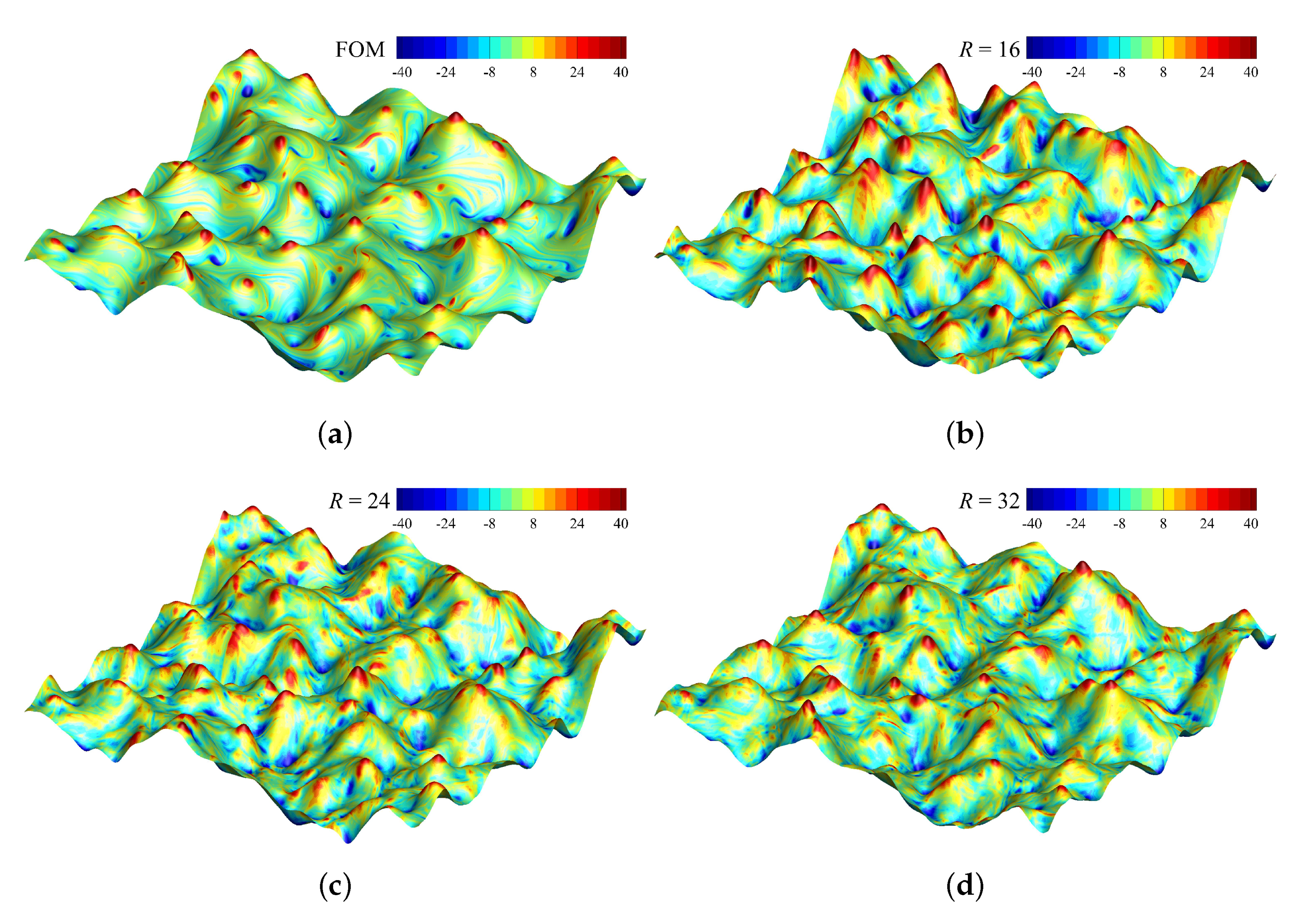
More visualizations of ROM’s predictability are provided in Figure 5 and Figure 6, showing the vorticity (in color) and streamfunction (in height) at the final time (i.e., t = 4 ), compared to the FOM results. In Figure 5, we illustrate that ROM with P = 1 fails to correctly predict the final fields at different values of R. At R = 16 , even the large scales are not captured accurately (recall the larger deviation of α 1 at final time from Figure 4). Conversely, both the large fine scales are predicted reliably using the partitioned ROM approach as shown in Figure 6 with R = 16 .
In order to obtain more insights about the scales resolved by partitioned ROM, compared to standard POD-based ROM, we compare PID ROM results for P = 8 and R = 16 , with standard ROM (i.e., P = 1 ) and increased number of modes. The root-mean-squares errors between Galerkin ROMs and FOM are shown in Table 1. We find that at least around R = 128 modes are needed for standard Galerkin ROM to achieve similar accuracy as partitioned ROM, which suggests that the relevant scales represented in those global 128 modes are almost encapsulated in 16 local modes if eight partitions are used. The computational gain of the PID approach can be easily seen from this analysis since online computational cost scales with O ( R 3 ) .

5.1. Kolmogorov n-Width and Relative Information Content

The Kologorov n-width provides a measure of the system’s reducibility, and in POD/PID context, it can be considered as a measure of how well a linear superposition of POD modes might represent the underlying dynamics. Similarly, a relative information content (RIC) of the snapshot matrix can be used as a simple quantitative metric to understand the Kolmogorov n-width of the system. The following RIC formula [105] is used to compute the percentage modal energy,
RIC ( l ) ( k ) = j = 1 k λ j ( l ) j = 1 N s / P λ j ( l ) × 100 .
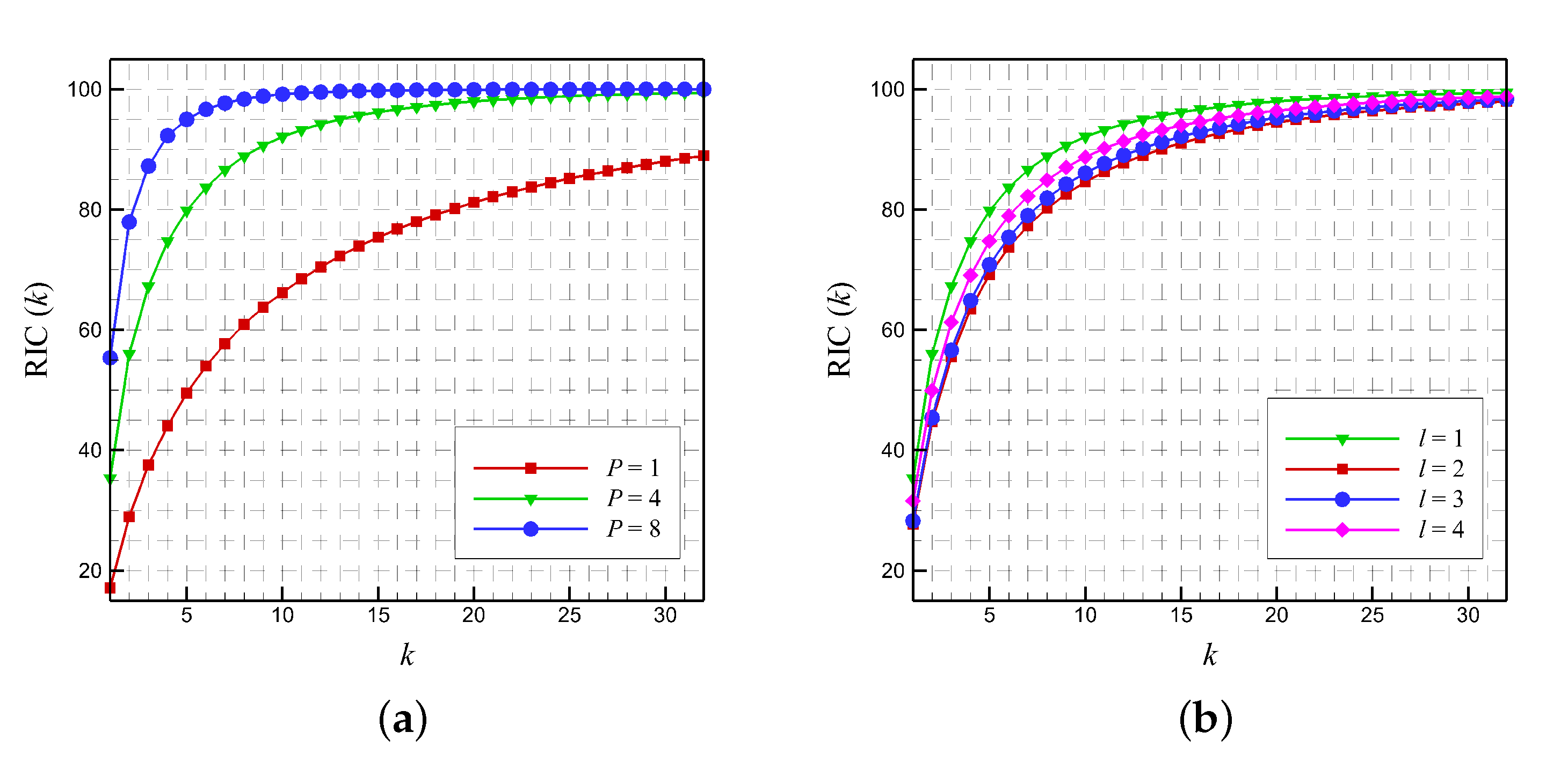
In other words, RIC ( k ) represents the fraction of information (variance) of the snapshot matrix that can be recovered using a specific number (k) of basis functions. Figure 7 shows the growth of RIC values with increasing k for different values of P. We can observe that, in case of P = 1 , the increase of the fraction of preserved information is relatively slow and more modes are required to exceed a 90 % RIC. On the other hand, with the use of a partitioned ROM approach, the slope of RIC curve increases significantly. For example, less than 10 modes are enough to hit the 90 % RIC value. In Kolmogorov n-width context, a faster increase in RIC corresponds to a faster decrease of the Kolmogorov n-width. Therefore, we consider that partitioned ROM can, in turn, help to break the Kolmogorov barrier and increase the system’s reducibility.
We note that, in Figure 7a, we only show the RIC in the first sub-interval (i.e., l = 1 ) for the sake of clarity. In Figure 7b, we plot the RIC curves for P = 4 in the four sub-intervals, where they almost match each other. An interesting observation from Figure 7b is that the slopes of RIC in the second and third sub-intervals are the lowest, compared to those in the first and last sub-intervals. This might be justified by the fact that flow is just initiated in the first sub-interval with relatively smooth dynamics. After that, most of the system’s vortical evolution and energy exchange take place within the following sub-intervals, decaying to quasi steady-state in the last sub-interval. For fast evolution and strong dynamics, more modes are required to capture sufficient amount of information. Alternatively, constructing local modes (through further partitioning) can help to accurately capture those dynamics. Since we use fixed number of modes in each sub-interval, this might correspond to different RIC values. That is the ROM approximation in some regions might be more or less accurate than the approximation in other regions. This might be crucial for flow problems with stronger and more complicated dynamics, where that difference in RIC values can cause inconsistencies of approximations. Alternatively, varying values of R can be used to satisfy pre-determined level of RIC in each partition.

5.2. Closure Modeling

It turns out that the partitioning approach helps with building more accurate and stable ROM due to several effects. First, it helps to construct more compact and localized subspaces which capture fine scales efficiently. Second, the energy (information) is concentrated in fewer modes. As a result of these two effects, modal truncation works effectively as the discarded modes have negligible effects on the system’s dynamics. However, as shown in previous discussions, a large number of partitions might be needed to provide acceptable accuracy. Other than the increased storage requirement to store basis function for each sub-interval, a projection error is accumulated due to interface treatment. If the true field data are available at the interface, it can be projected onto the respective basis functions to obtain the corresponding modal coefficients at the beginning of the sub-interval. Since this is not generally available, the update of ROM solution manifold is performed using Equation (27), where the obtained reduced order approximation of the field from the previous partition is projected onto the basis functions of the following partition. Since that approximation depends on the accuracy of the ROM in the current partition, and lives in a reduced subspace different than that of the following subspace, discontinuities can easily occur at the interface. In Figure 8, we show the modal coefficients at the interfaces for P = 4 obtained from ROMs with different R dimensions. Moreover, the mismatch between initial conditions at each interface increases in subsequent partitions, due to the successive interface treatment, resulting in amplification of the error. However, we highlight that the projection error generated at the interface is bounded and overall accuracy gain due to the localization in the PID approach surpasses that error.
Conversely, for ROM with global POD application without any partitioning, the truncated modes might include substantial amount of energy and/or have strong interactions with the retained modes. Hence, inaccuracies and instabilities can easily take place in the produced ROM. Therefore, a compromise between accuracy gain from localization and projection error from interfaces should be considered while selecting the number of intervals. To enhance the stability of ROMs, closure models have been effectively incorporated (inspired from large eddy simulation (LES) studies). Here, we investigate the effect of closure modeling to stabilize and correct ROMs based on global application of POD (i.e., P = 1 ). We utilize a linear mode length eddy viscosity closure based on Rempfer’s model [72,106,107], where the 2D Navier–Stokes equation (given in Equation (2)) is re-written as
ω t + J ( ω , ψ ) = 1 Re 1 + κ k R 2 ω ,
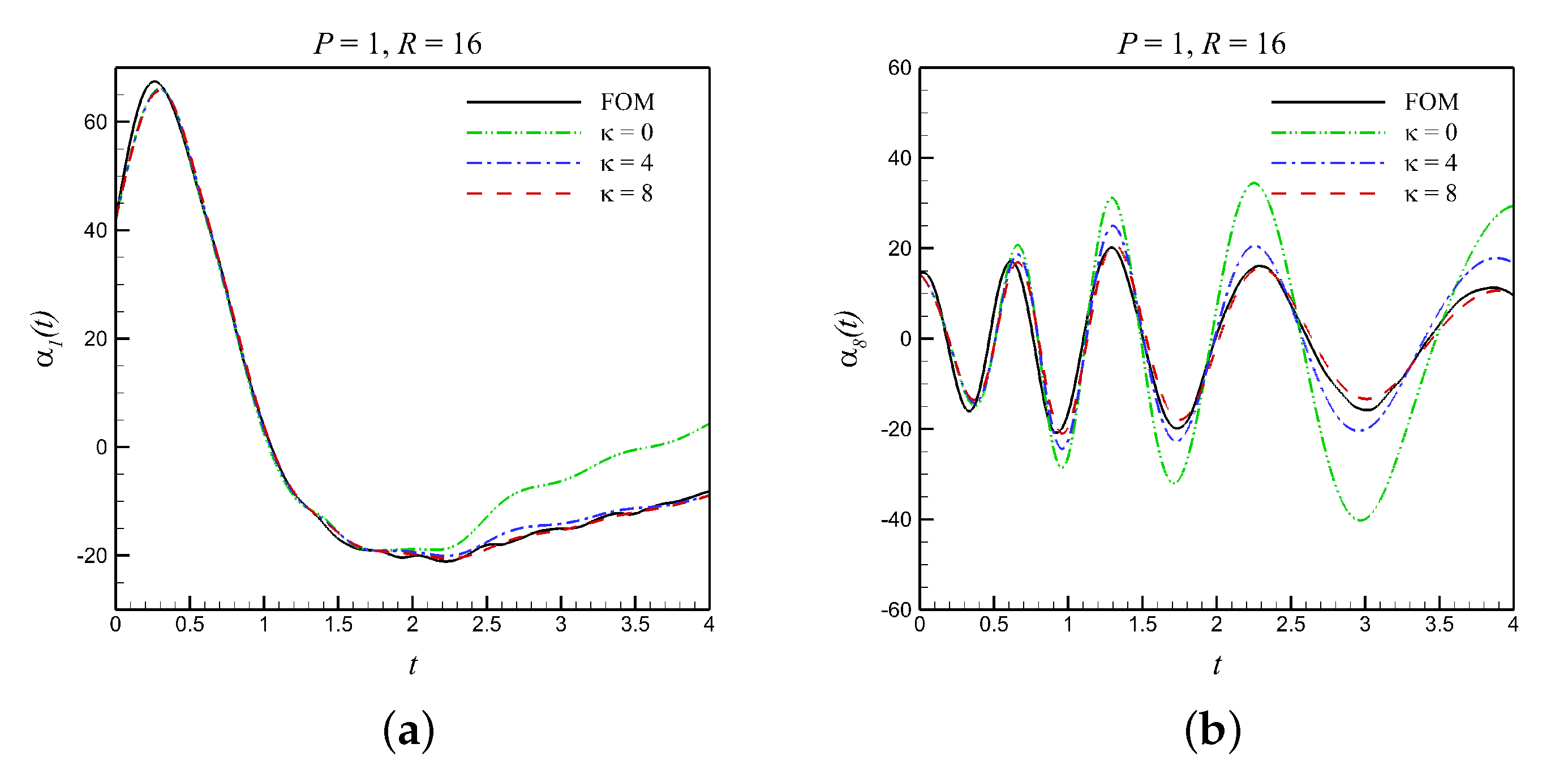
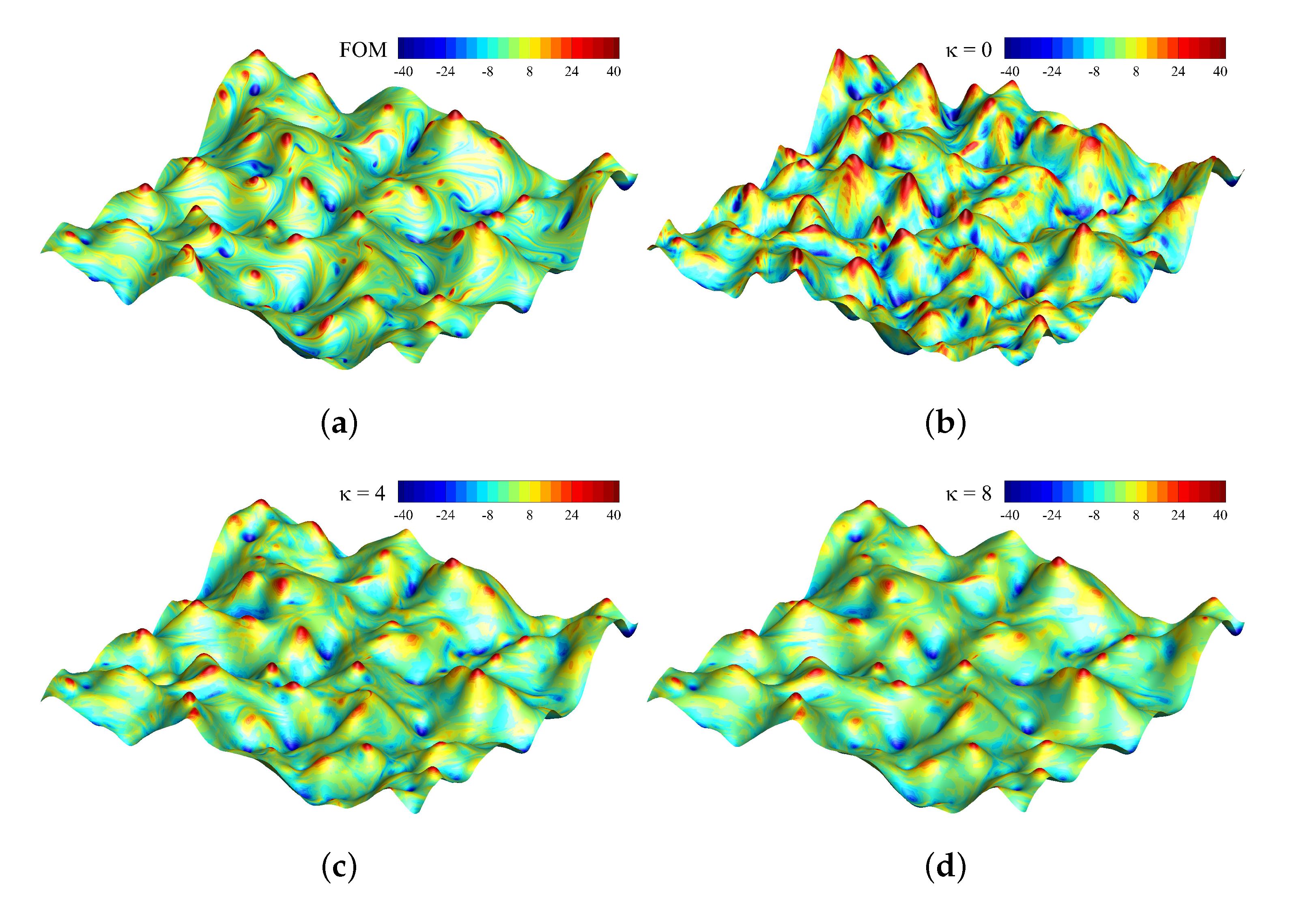
where κ is a free-parameter controlling the amount of stabilization added to the model, R is the number of modes, and k is the mode index (i.e., k = 1 , 2 , , R ). More recently, several ideas from a plethora of predictive turbulence models have been used in ROMs in the spirit of closure modeling to account for the effects of the truncated scales [108,109,110,111,112,113,114,115]. In the present study, we test the effect of the linear mode dependent eddy viscosity closure model for κ { 0 , 4 , 8 } , where κ = 0 corresponds to the standard Galerkin ROM without stabilization.
In Figure 9, we present the temporal evolution of α 1 and α 8 for ROM with 16 modes and a single global interval (i.e., P = 1 ). We find that the closure significantly improves the predictive capabilities of the ROM, and with increasing κ (i.e., adding more stabilization), results converge to the true values of the modal coefficients.
In addition, the final vorticity and streamfunction fields at t = 4 are shown in Figure 10. We can notice tremendous improvement of predicted results with closure modeling. With close investigation of surface topology, we can observe that Figure 10d captures the correct large scales as Figure 10a. However, we can see that smaller and finer details are overlooked and smoothed-out. This is to be expected given the fact that closure models try to compensate the effect of the truncated modes on the dynamics of the retained modes. In other words, it helps to improve our predictions of the dynamics of these retained modes, but does not add the contribution of the truncated modes into our reduced order approximation. Therefore, our ROM prediction will always be restricted to the scales represented by the retained modes. In case of global POD modes, only the large scales are captured and the fine scales are smoothed-out, which justifies Figure 10d.
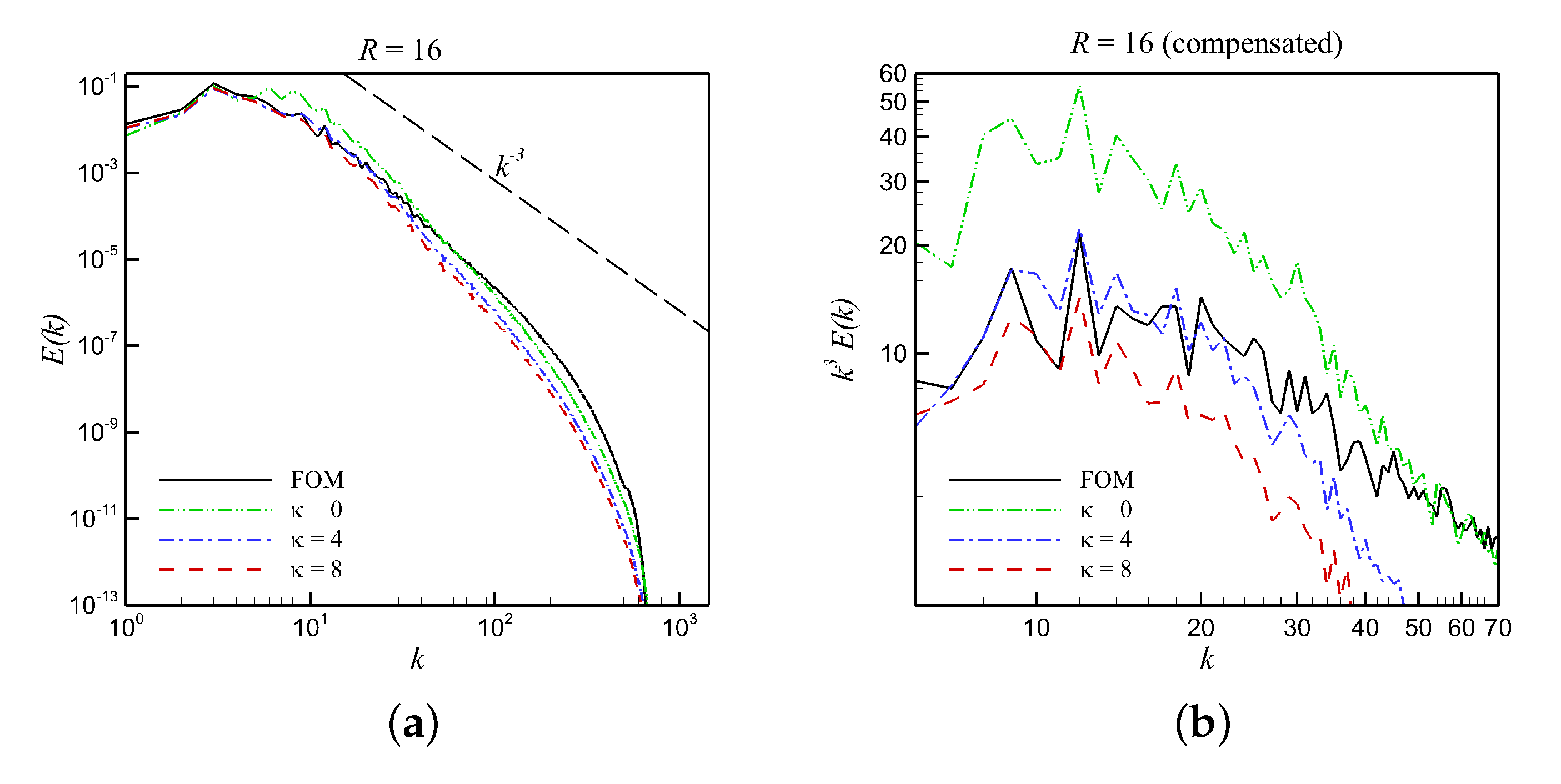
Finally, the energy spectrum at final time is given in Figure 11, where we can see the influence of closure modeling in improving ROM results. A very nice observation from this figure is that stabilization helps a lot in the inertial regime of energy spectrum, but it causes over-stabilization in the dissipative regime.
The root-mean-squares errors (RMSE) between Galerkin ROM approximation (with P = 1 and R = 16 ), in the presence of stabilization, and FOM solution are shown in Table 2, compared to the base case without closure. It is clear that the addition of stabilization to Galerkin ROM helps to improve the predictions and reduces the approximation error. However, compared to Table 1, we can deduce that the accuracy gain due to partitioning is much more superior than that of closure. In addition, the RMSE is sensitive to the value of the stabilization parameter. Therefore, a dynamic selection of this parameter might be needed to guarantee sufficient correction.
Moreover, it should be noted that there might exist situations where the gain from only closure is minimum, even in case of “optimal” closure [73]. Hence, a combination of both partitioning and stabilization seems to be a feasible choice for building accurate, stable, and compact ROMs for turbulent flows. Indeed, Ahmed and San [72] demonstrated that an eddy viscosity based closure in conjunction with PID yields significant improvements in accuracy for capturing strong moving discontinuities with a negligibly small computational overhead. In addition, Table 3 shows the effect of stabilization through closure modeling in the partitioned ROM (with P = and R = 16 ). It is clear that the closure slightly improves the RMSE of vorticity field approximation. In addition, we can see that further increase in κ can actually increase the RMSE due to over stabilization. It can be also observed that RMSE in streamfunction predictions in case of closure modeling with PID is generally larger than that in case of PID without closure. This can be attributed to the nature of streamfunction being inverse of the Laplacian operator of vorticity, making it a smoother field by construction. Therefore, closure with PID might cause over-stabilization and excessive smoothing of the streamfunction fields predictions. This again suggests the development of a dynamical strategy to estimate optimal values of eddy viscosity coefficient.

5.3. Computational Cost

In addition to the accuracy gains through the partitioned ROM approach, presented in previous subsections, a comparison in terms of computational cost is required for fair assessment. Here, we consider two phases of ROM computations: offline and online. By offline, we refer to the evaluation of the vectors, matrices, and tensors corresponding to the constant, linear, and nonlinear predetermined model coefficients (i.e., B , L , and R ). Meanwhile, we denote the actual prediction and solution of Equation (21) as the online stage. Table 4 provides the CPU times in the offline and online stages for different number of partitions and modes. From this table, we can see that increasing the number of modes increases the CPU times for both the offline (due to computation of larger vectors, matrices, and tensors) and online (due to solving an increased number of equations) stages. Interestingly, we can observe that the computational cost of the online stage scales cubically with increasing R. This conforms to the quadratic nonlinearity in the investigated system, making the online cost an order of O ( R 3 ) .
On the other hand, increasing the number of partitions has a negligible effect on the online CPU time. Therefore, the partitioned ROM approach provides more accurate results with similar online costs as standard ROM with the same number of modes. However, increasing P (with fixed R) results in an increase in the offline CPU time. This corresponds to the computation of B , L , and R for each individual partition. That is why the offline CPU time scales linearly with increasing P. Nonetheless, it was shown in [73] that the CPU times for basis construction are largely reduced in the PID framework due to the solution of smaller eigenvalue problems rather than solving a large one. Finally, it is noteworthy that the partitioned ROM approach requires more memory to store the local basis functions and model predetermined coefficients in each partition. Therefore, we can consider that partitioned ROM converts the offline and storage costs into a speed-up of the online deployment.

6. Conclusions and Future Works

We utilize a partitioning approach in the current study in order to build a compact reduced order models of 2D turbulent flows. We demonstrate the framework using the two-dimensional decaying Kraichnan turbulence. It is shown that this partitioned ROM helps to break the Kolmogorov n-width barrier, in the context of a relative information content criterion. An energy spectrum analysis is performed to emphasize the capabilities of the presented framework to sufficiently capture both the large and fine scales and recover the energy spectra within the inertial and dissipative ranges. The partitioned ROM produces significantly more accurate predictions than standard ROM without partitioning. A computational CPU time analysis reveals that the partitioned ROM minimizes the online cost at the expense of offline cost and increased memory to build reduced order approximation with acceptable accuracy. In addition, we investigate the use of a linear mode dependent eddy viscosity to stabilize ROM prediction. We find that closure improves the results in the inertial kinetic energy regime, corresponding to the large scales. However, it presents over-stabilization in the dissipative regime, which smoothens out the field finer details. This might advocate a strategy to develop optimal (or near optimal) estimates for the eddy viscosity coefficients to be posed. Therefore, we suggest the use of partitioning along with closure as an enabler for more efficient ROMs turbulent flow systems. Incorporating PID with closure would provide the flexibility of constructing ROMs with less modes (and same number of partitions), or with less partitions (and same number of modes). The former would provide higher speed-ups during online deployment, while the latter would reduce the offline cost.
To this end, the partitioned ROM has been shown to improve the predictions for the investigated 2D Kraichnan turbulence case. However, scaling this framework into a 3D setting is still required to fully assess the validity of the framework to address realistic turbulent flows with strong anisotropy. In addition, the PID has been shown to capture finer details than standard global POD. Application of this approach onto flow situations where global basis fails drastically and results in completely unstable and inaccurate ROMs can be an interesting extension to the current study. Also, the adopted PID approach assumes evenly-spaced partitions with an equal number of modes. Despite the resulting simplicity of implementation, this fixed partitioning might be less meaningful for more challenging flow problems where dynamics change rapidly. Therefore, an adaptive partitioning with varying number of modes can be another extension to generalize the present work. The assumption of non-overlapping partitions might also be relaxed to allow overlapping sub-intervals with an indicator for smooth transition between partitions based on the actual flow conditions. Finally, the development of a strategy to dynamically update the basis functions using data assimilation techniques would enable the extrapolation of ROM in time while reflecting local phenomena.

Author Contributions

Data curation, S.E.A. and O.S.; Supervision, O.S.; Writing—original draft, S.E.A.; and Writing—review and editing, S.E.A. and O.S. All authors have read and agreed to the published version of the manuscript.

Funding

U.S. Department of Energy, Office of Science, Office of Advanced Scientific Computing Research, Award Number: DE-SC0019290.

Acknowledgments

This material is based upon work supported by the U.S. Department of Energy, Office of Science, Office of Advanced Scientific Computing Research under Award Number DE-SC0019290. Omer San gratefully acknowledges their support. Disclaimer: This report was prepared as an account of work sponsored by an agency of the United States Government. Neither the United States Government nor any agency thereof, nor any of their employees, makes any warranty, express or implied, or assumes any legal liability or responsibility for the accuracy, completeness, or usefulness of any information, apparatus, product, or process disclosed, or represents that its use would not infringe privately owned rights. Reference herein to any specific commercial product, process, or service by trade name, trademark, manufacturer, or otherwise does not necessarily constitute or imply its endorsement, recommendation, or favoring by the United States Government or any agency thereof. The views and opinions of authors expressed herein do not necessarily state or reflect those of the United States Government or any agency thereof.

Conflicts of Interest

The authors declare no conflict of interest.

References

  1. Powell, J.R. The quantum limit to Moore’s law. Proc. IEEE 2008, 96, 1247–1248. [Google Scholar] [CrossRef]
  2. Waldrop, M.M. The chips are down for Moore’s law. Nat. News 2016, 530, 144. [Google Scholar] [CrossRef] [PubMed] [Green Version]
  3. Kumar, S. The end of Moore’s law and reinventing computing. In High-Speed and Lower Power Technologies: Electronics and Photonics; Choi, J.H., Ed.; CRC Press: Boca Raton, FL, USA, 2018. [Google Scholar]
  4. Taira, K.; Brunton, S.L.; Dawson, S.T.; Rowley, C.W.; Colonius, T.; McKeon, B.J.; Schmidt, O.T.; Gordeyev, S.; Theofilis, V.; Ukeiley, L.S. Modal analysis of fluid flows: An overview. AIAA J. 2017, 55, 4013–4041. [Google Scholar] [CrossRef] [Green Version]
  5. Puzyrev, V.; Ghommem, M.; Meka, S. pyROM: A computational framework for reduced order modeling. J. Comput. Sci. 2019, 30, 157–173. [Google Scholar] [CrossRef]
  6. Rasheed, A.; San, O.; Kvamsdal, T. Digital Twin: Values, Challenges and Enablers. arXiv 2019, arXiv:1910.01719. [Google Scholar]
  7. Grieves, M.; Vickers, J. Digital twin: Mitigating unpredictable, undesirable emergent behavior in complex systems. In Transdisciplinary Perspectives on Complex Systems; Springer: Berlin/Heidelberg, Germany, 2017; pp. 85–113. [Google Scholar]
  8. Boschert, S.; Rosen, R. Digital twin—The simulation aspect. In Mechatronic Futures; Springer: Berlin/Heidelberg, Germany, 2016; pp. 59–74. [Google Scholar]
  9. Tao, F.; Cheng, J.; Qi, Q.; Zhang, M.; Zhang, H.; Sui, F. Digital twin-driven product design, manufacturing and service with big data. Int. J. Adv. Manuf. Technol. 2018, 94, 3563–3576. [Google Scholar] [CrossRef]
  10. Uhlemann, T.H.J.; Lehmann, C.; Steinhilper, R. The digital twin: Realizing the cyber-physical production system for industry 4.0. Procedia CIRP 2017, 61, 335–340. [Google Scholar] [CrossRef]
  11. Glaessgen, E.; Stargel, D. The digital twin paradigm for future NASA and US Air Force vehicles. In Proceedings of the 53rd AIAA/ASME/ASCE/AHS/ASC Structures, Structural Dynamics and Materials Conference 20th AIAA/ASME/AHS Adaptive Structures Conference 14th AIAA, Honolulu, HI, USA, 23–26 April 2012; p. 1818. [Google Scholar]
  12. Kapteyn, M.G.; Willcox, K.; Knezevic, D.J. Toward predictive digital twins via component-based reduced-order models and interpretable machine learning. In Proceedings of the AIAA Scitech 2020 Forum, Orlando, FL, USA, 6–10 January 2020; p. 0418. [Google Scholar]
  13. Singh, V.; Willcox, K.E. Engineering Design with Digital Thread. AIAA J. 2018, 56, 4515–4528. [Google Scholar] [CrossRef]
  14. Hartmann, D.; Herz, M.; Wever, U. Model order reduction a key technology for digital twins. In Reduced-Order Modeling (ROM) for Simulation and Optimization; Springer: Berlin/Heidelberg, Germany, 2018; pp. 167–179. [Google Scholar]
  15. Noack, B.R.; Morzynski, M.; Tadmor, G. Reduced-Order Modelling for Flow Control; Springer: Berlin/Heidelberg, Germany, 2011; Volume 528. [Google Scholar]
  16. Ito, K.; Ravindran, S.S. Reduced basis method for optimal control of unsteady viscous flows. Int. J. Comput. Fluid Dyn. 2001, 15, 97–113. [Google Scholar] [CrossRef]
  17. McNamara, A.; Treuille, A.; Popović, Z.; Stam, J. Fluid control using the adjoint method. ACM Trans. Graph. 2004, 23, 449–456. [Google Scholar] [CrossRef]
  18. Bergmann, M.; Cordier, L. Optimal control of the cylinder wake in the laminar regime by trust-region methods and POD reduced-order models. J. Comput. Phys. 2008, 227, 7813–7840. [Google Scholar] [CrossRef] [Green Version]
  19. Ravindran, S.S. A reduced-order approach for optimal control of fluids using proper orthogonal decomposition. Int. J. Numer. Methods Fluids 2000, 34, 425–448. [Google Scholar] [CrossRef]
  20. Graham, W.; Peraire, J.; Tang, K. Optimal control of vortex shedding using low-order models. Part I–open-loop model development. Int. J. Numer. Methods Eng. 1999, 44, 945–972. [Google Scholar] [CrossRef]
  21. Graham, W.; Peraire, J.; Tang, K. Optimal control of vortex shedding using low-order models. Part II–model-based control. Int. J. Numer. Methods Eng. 1999, 44, 973–990. [Google Scholar] [CrossRef]
  22. Brunton, S.L.; Noack, B.R. Closed-loop turbulence control: Progress and challenges. Appl. Mech. Rev. 2015, 67, 050801. [Google Scholar] [CrossRef]
  23. Daescu, D.N.; Navon, I.M. Efficiency of a POD-based reduced second-order adjoint model in 4D-Var data assimilation. Int. J. Numer. Methods Fluids 2007, 53, 985–1004. [Google Scholar] [CrossRef] [Green Version]
  24. Navon, I.M. Data assimilation for numerical weather prediction: A review. In Data Assimilation for Atmospheric, Oceanic and Hydrologic Applications; Park, S.K., Xu, L., Eds.; Springer: New York, NY, USA, 2009; pp. 21–65. [Google Scholar]
  25. Cao, Y.; Zhu, J.; Navon, I.M.; Luo, Z. A reduced-order approach to four-dimensional variational data assimilation using proper orthogonal decomposition. Int. J. Numer. Methods Fluids 2007, 53, 1571–1583. [Google Scholar] [CrossRef]
  26. He, J.; Sarma, P.; Durlofsky, L.J. Use of reduced-order models for improved data assimilation within an EnKF context. In Proceedings of the SPE Reservoir Simulation Symposium, The Woodlands, TX, USA, 21–23 February 2011; Society of Petroleum Engineers: Richardson, TX, USA, 2011. [Google Scholar]
  27. Houtekamer, P.L.; Mitchell, H.L. Data assimilation using an ensemble Kalman filter technique. Mon. Weather. Rev. 1998, 126, 796–811. [Google Scholar] [CrossRef]
  28. Houtekamer, P.L.; Mitchell, H.L. A sequential ensemble Kalman filter for atmospheric data assimilation. Mon. Weather. Rev. 2001, 129, 123–137. [Google Scholar] [CrossRef]
  29. Bennett, A.F. Inverse Modeling of the Ocean and Atmosphere; Cambridge University Press: New York, NY, USA, 2005. [Google Scholar]
  30. Evensen, G. Data Assimilation: The Ensemble Kalman Filter; Springer: Berlin/Heidelberg, Germany, 2009. [Google Scholar]
  31. Law, K.J.; Stuart, A.M. Evaluating data assimilation algorithms. Mon. Weather. Rev. 2012, 140, 3757–3782. [Google Scholar] [CrossRef] [Green Version]
  32. Buljak, V. Inverse Analyses with Model Reduction: Proper Orthogonal Decomposition in Structural Mechanics; Springer: Berlin/Heidelberg, Germany, 2011. [Google Scholar]
  33. Xiao, D.; Du, J.; Fang, F.; Pain, C.; Li, J. Parameterised non-intrusive reduced order methods for ensemble Kalman filter data assimilation. Comput. Fluids 2018, 177, 69–77. [Google Scholar] [CrossRef]
  34. Navon, I. Practical and theoretical aspects of adjoint parameter estimation and identifiability in meteorology and oceanography. Dyn. Atmos. Ocean. 1998, 27, 55–79. [Google Scholar] [CrossRef] [Green Version]
  35. Fu, H.; Wang, H.; Wang, Z. POD/DEIM reduced-order modeling of time-fractional partial differential equations with applications in parameter identification. J. Sci. Comput. 2018, 74, 220–243. [Google Scholar] [CrossRef] [Green Version]
  36. Boulakia, M.; Schenone, E.; Gerbeau, J.F. Reduced-order modeling for cardiac electrophysiology. Application to parameter identification. Int. J. Numer. Methods Biomed. Eng. 2012, 28, 727–744. [Google Scholar] [CrossRef] [PubMed] [Green Version]
  37. Kramer, B.; Peherstorfer, B.; Willcox, K. Feedback control for systems with uncertain parameters using online-adaptive reduced models. SIAM J. Appl. Dyn. Syst. 2017, 16, 1563–1586. [Google Scholar] [CrossRef] [Green Version]
  38. Galbally, D.; Fidkowski, K.; Willcox, K.; Ghattas, O. Non-linear model reduction for uncertainty quantification in large-scale inverse problems. Int. J. Numer. Methods Eng. 2010, 81, 1581–1608. [Google Scholar] [CrossRef] [Green Version]
  39. Biegler, L.; Biros, G.; Ghattas, O.; Heinkenschloss, M.; Keyes, D.; Mallick, B.; Tenorio, L.; Waanders, B.V.B.; Willcox, K.; Marzouk, Y. Large-Scale Inverse Problems and Quantification of Uncertainty; Wiley Online Library: Chichester, UK, 2011. [Google Scholar]
  40. Mathelin, L.; Hussaini, M.Y.; Zang, T.A. Stochastic approaches to uncertainty quantification in CFD simulations. Numer. Algorithms 2005, 38, 209–236. [Google Scholar] [CrossRef]
  41. Smith, R.C. Uncertainty Quantification: Theory, Implementation, and Applications; SIAM: Philadelphia, PA, USA, 2014. [Google Scholar]
  42. Najm, H.N. Uncertainty quantification and polynomial chaos techniques in computational fluid dynamics. Annu. Rev. Fluid Mech. 2009, 41, 35–52. [Google Scholar] [CrossRef]
  43. Zahr, M.J.; Carlberg, K.T.; Kouri, D.P. An efficient, globally convergent method for optimization under uncertainty using adaptive model reduction and sparse grids. SIAM/ASA J. Uncertain. Quantif. 2019, 7, 877–912. [Google Scholar] [CrossRef]
  44. Fairbanks, H.R.; Jofre, L.; Geraci, G.; Iaccarino, G.; Doostan, A. Bi-fidelity approximation for uncertainty quantification and sensitivity analysis of irradiated particle-laden turbulence. J. Comput. Phys. 2020, 402, 108996. [Google Scholar] [CrossRef] [Green Version]
  45. Kevlahan, N.R.; Hunt, J.; Vassilicos, J. A comparison of different analytical techniques for identifying structures in turbulence. Appl. Sci. Res. 1994, 53, 339–355. [Google Scholar] [CrossRef] [Green Version]
  46. Holmes, P.; Lumley, J.L.; Berkooz, G. Turbulence, Coherent Structures, Dynamical Systems and Symmetry; Cambridge University Press: New York, NY, USA, 1998. [Google Scholar]
  47. Rowley, C.W.; Colonius, T.; Murray, R.M. Model reduction for compressible flows using POD and Galerkin projection. Phys. D Nonlinear Phenom. 2004, 189, 115–129. [Google Scholar] [CrossRef]
  48. Ma, Z.; Ahuja, S.; Rowley, C.W. Reduced-order models for control of fluids using the eigensystem realization algorithm. Theor. Comput. Fluid Dyn. 2011, 25, 233–247. [Google Scholar] [CrossRef] [Green Version]
  49. Rowley, C.W. Model reduction for fluids, using balanced proper orthogonal decomposition. Int. J. Bifurc. Chaos 2005, 15, 997–1013. [Google Scholar] [CrossRef] [Green Version]
  50. Willcox, K.; Peraire, J. Balanced model reduction via the proper orthogonal decomposition. AIAA J. 2002, 40, 2323–2330. [Google Scholar] [CrossRef]
  51. Schmid, P.J. Dynamic mode decomposition of numerical and experimental data. J. Fluid Mech. 2010, 656, 5–28. [Google Scholar] [CrossRef] [Green Version]
  52. Williams, M.O.; Kevrekidis, I.G.; Rowley, C.W. A data–driven approximation of the koopman operator: Extending dynamic mode decomposition. J. Nonlinear Sci. 2015, 25, 1307–1346. [Google Scholar] [CrossRef] [Green Version]
  53. Peterson, J.S. The reduced basis method for incompressible viscous flow calculations. SIAM J. Sci. Stat. Comput. 1989, 10, 777–786. [Google Scholar] [CrossRef]
  54. Sirovich, L. Turbulence and the dynamics of coherent structures. I. Coherent structures. Q. Appl. Math. 1987, 45, 561–571. [Google Scholar] [CrossRef] [Green Version]
  55. Rim, D.; Peherstorfer, B.; Mandli, K.T. Manifold Approximations via Transported Subspaces: Model reduction for transport-dominated problems. arXiv 2019, arXiv:1912.13024. [Google Scholar]
  56. Lai, X.; Wang, X.; Nie, Y.; Li, Q. Characterizing complex flows via adaptive sparse dynamic mode decomposition with error approximation. Int. J. Numer. Methods Fluids 2019. [Google Scholar] [CrossRef]
  57. Kastian, S.; Reese, S. An Adaptive Way of Choosing Significant Snapshots for Proper Orthogonal Decomposition. In Proceedings of the IUTAM Symposium on Model Order Reduction of Coupled Systems, Stuttgart, Germany, 22–25 May 2018; Springer: Berlin/Heidelberg, Germany, 2020; pp. 67–79. [Google Scholar]
  58. Aubry, N.; Holmes, P.; Lumley, J.L.; Stone, E. The dynamics of coherent structures in the wall region of a turbulent boundary layer. J. Fluid Mech. 1988, 192, 115–173. [Google Scholar] [CrossRef]
  59. Wang, Z.; Akhtar, I.; Borggaard, J.; Iliescu, T. Proper orthogonal decomposition closure models for turbulent flows: A numerical comparison. Comput. Methods Appl. Mech. Eng. 2012, 237, 10–26. [Google Scholar] [CrossRef] [Green Version]
  60. Carlberg, K.; Farhat, C.; Cortial, J.; Amsallem, D. The GNAT method for nonlinear model reduction: Effective implementation and application to computational fluid dynamics and turbulent flows. J. Comput. Phys. 2013, 242, 623–647. [Google Scholar] [CrossRef] [Green Version]
  61. Protas, B.; Noack, B.R.; Östh, J. Optimal nonlinear eddy viscosity in Galerkin models of turbulent flows. J. Fluid Mech. 2015, 766, 337–367. [Google Scholar] [CrossRef] [Green Version]
  62. Stabile, G.; Ballarin, F.; Zuccarino, G.; Rozza, G. A reduced order variational multiscale approach for turbulent flows. Adv. Comput. Math. 2019, 45, 2349–2368. [Google Scholar] [CrossRef] [Green Version]
  63. Xiao, D.; Heaney, C.; Mottet, L.; Fang, F.; Lin, W.; Navon, I.; Guo, Y.; Matar, O.; Robins, A.; Pain, C. A reduced order model for turbulent flows in the urban environment using machine learning. Build. Environ. 2019, 148, 323–337. [Google Scholar] [CrossRef] [Green Version]
  64. Xiao, D.; Heaney, C.; Fang, F.; Mottet, L.; Hu, R.; Bistrian, D.; Aristodemou, E.; Navon, I.; Pain, C. A domain decomposition non-intrusive reduced order model for turbulent flows. Comput. Fluids 2019, 182, 15–27. [Google Scholar] [CrossRef] [Green Version]
  65. Kolmogoroff, A. Über die beste Annäherung von Funktionen einer gegebenen Funktionenklasse. Ann. Math. 1936, 37, 107–110. [Google Scholar] [CrossRef]
  66. Pinkus, A. N-Widths in Approximation Theory; Springer Science & Business Media: Berlin/Heidelberg, Germany, 2012; Volume 7. [Google Scholar]
  67. Taddei, T. A registration method for model order reduction: Data compression and geometry reduction. arXiv 2019, arXiv:1906.11008. [Google Scholar]
  68. Greif, C.; Urban, K. Decay of the Kolmogorov N-width for wave problems. Appl. Math. Lett. 2019, 96, 216–222. [Google Scholar] [CrossRef] [Green Version]
  69. IJzerman, W. Signal Representation and Modeling of Spatial Structures in Fluids. Ph.D. Thesis, University of Twente, Enschede, The Netherlands, 2000. [Google Scholar]
  70. Borggaard, J.; Hay, A.; Pelletier, D. Interval-based reduced order models for unsteady fluid flow. Int. J. Numer. Anal. Model. 2007, 4, 353–367. [Google Scholar]
  71. San, O.; Borggaard, J. Principal interval decomposition framework for POD reduced-order modeling of convective Boussinesq flows. Int. J. Numer. Methods Fluids 2015, 78, 37–62. [Google Scholar] [CrossRef]
  72. Ahmed, M.; San, O. Stabilized principal interval decomposition method for model reduction of nonlinear convective systems with moving shocks. Comput. Appl. Math. 2018, 37, 6870–6902. [Google Scholar] [CrossRef]
  73. Ahmed, S.E.; Rahman, S.M.; San, O.; Rasheed, A.; Navon, I.M. Memory embedded non-intrusive reduced order modeling of non-ergodic flows. Phys. Fluids 2019, 31, 126602. [Google Scholar] [CrossRef] [Green Version]
  74. Charney, J.G. Geostrophic turbulence. J. Atmos. Sci. 1971, 28, 1087–1095. [Google Scholar] [CrossRef] [Green Version]
  75. Kraichnan, R.H.; Montgomery, D. Two-dimensional turbulence. Rep. Prog. Phys. 1980, 43, 547. [Google Scholar] [CrossRef]
  76. Boffetta, G.; Ecke, R.E. Two-dimensional turbulence. Annu. Rev. Fluid Mech. 2012, 44, 427–451. [Google Scholar] [CrossRef]
  77. Rempfer, D. On low-dimensional Galerkin models for fluid flow. Theor. Comput. Fluid Dyn. 2000, 14, 75–88. [Google Scholar] [CrossRef]
  78. Zhang, M.; Stevens, R.J. Characterizing the Coherent Structures Within and Above Large Wind Farms. Bound.-Layer Meteorol. 2019, 1–20. [Google Scholar] [CrossRef] [Green Version]
  79. Shah, S.; Bou-Zeid, E. Very-large-scale motions in the atmospheric boundary layer educed by snapshot proper orthogonal decomposition. Bound.-Layer Meteorol. 2014, 153, 355–387. [Google Scholar] [CrossRef]
  80. Östh, J.; Noack, B.R.; Krajnović, S.; Barros, D.; Borée, J. On the need for a nonlinear subscale turbulence term in POD models as exemplified for a high-Reynolds-number flow over an Ahmed body. J. Fluid Mech. 2014, 747, 518–544. [Google Scholar] [CrossRef] [Green Version]
  81. Grimberg, S.; Farhat, C.; Youkilis, N. On the stability of projection-based model order reduction for convection-dominated laminar and turbulent flows. arXiv 2020, arXiv:2001.10110. [Google Scholar]
  82. Carlberg, K.; Barone, M.; Antil, H. Galerkin v. least-squares Petrov–Galerkin projection in nonlinear model reduction. J. Comput. Phys. 2017, 330, 693–734. [Google Scholar] [CrossRef] [Green Version]
  83. Kraichnan, R.H. Inertial ranges in two-dimensional turbulence. Phys. Fluids 1967, 10, 1417–1423. [Google Scholar] [CrossRef] [Green Version]
  84. Batchelor, G.K. Computation of the energy spectrum in homogeneous two-dimensional turbulence. Phys. Fluids 1969, 12, II-233. [Google Scholar] [CrossRef]
  85. Leith, C. Atmospheric predictability and two-dimensional turbulence. J. Atmos. Sci. 1971, 28, 145–161. [Google Scholar] [CrossRef] [Green Version]
  86. San, O.; Staples, A.E. High-order methods for decaying two-dimensional homogeneous isotropic turbulence. Comput. Fluids 2012, 63, 105–127. [Google Scholar] [CrossRef] [Green Version]
  87. Arakawa, A. Computational design for long-term numerical integration of the equations of fluid motion: Two-dimensional incompressible flow. Part I. J. Comput. Phys. 1966, 1, 119–143. [Google Scholar] [CrossRef]
  88. Gottlieb, S.; Shu, C.W. Total variation diminishing Runge-Kutta schemes. Math. Comput. 1998, 67, 73–85. [Google Scholar] [CrossRef] [Green Version]
  89. Rowley, C.W.; Dawson, S.T. Model reduction for flow analysis and control. Annu. Rev. Fluid Mech. 2017, 49, 387–417. [Google Scholar] [CrossRef] [Green Version]
  90. Chen, K.K.; Tu, J.H.; Rowley, C.W. Variants of dynamic mode decomposition: Boundary condition, Koopman, and Fourier analyses. J. Nonlinear Sci. 2012, 22, 887–915. [Google Scholar] [CrossRef]
  91. Press, W.H.; Flannery, B.P.; Teukolsky, S.A.; Vetterling, W.T. Numerical Recipes in FORTRAN; Cambridge University Press: New York, NY, USA, 1992. [Google Scholar]
  92. Chaturantabut, S.; Sorensen, D.C. Discrete empirical interpolation for nonlinear model reduction. In Proceedings of the 48th IEEE Conference on Decision and Control, Shanghai, China, 16–18 December 2009; pp. 4316–4321. [Google Scholar]
  93. Chaturantabut, S.; Sorensen, D.C. Nonlinear model reduction via discrete empirical interpolation. SIAM J. Sci. Comput. 2010, 32, 2737–2764. [Google Scholar] [CrossRef]
  94. Everson, R.; Sirovich, L. Karhunen–Loeve procedure for gappy data. JOSA A 1995, 12, 1657–1664. [Google Scholar] [CrossRef] [Green Version]
  95. Astrid, P.; Weiland, S.; Willcox, K.; Backx, T. Missing point estimation in models described by proper orthogonal decomposition. IEEE Trans. Autom. Control. 2008, 53, 2237–2251. [Google Scholar] [CrossRef] [Green Version]
  96. Zimmermann, R.; Willcox, K. An accelerated greedy missing point estimation procedure. SIAM J. Sci. Comput. 2016, 38, A2827–A2850. [Google Scholar] [CrossRef] [Green Version]
  97. Ştefănescu, R.; Sandu, A.; Navon, I.M. Comparison of POD reduced order strategies for the nonlinear 2D shallow water equations. Int. J. Numer. Methods Fluids 2014, 76, 497–521. [Google Scholar] [CrossRef] [Green Version]
  98. Dimitriu, G.; Ştefănescu, R.; Navon, I.M. Comparative numerical analysis using reduced-order modeling strategies for nonlinear large-scale systems. J. Comput. Appl. Math. 2017, 310, 32–43. [Google Scholar] [CrossRef]
  99. Cazemier, W.; Verstappen, R.; Veldman, A. Proper orthogonal decomposition and low-dimensional models for driven cavity flows. Phys. Fluids 1998, 10, 1685–1699. [Google Scholar] [CrossRef] [Green Version]
  100. Amsallem, D.; Zahr, M.J.; Farhat, C. Nonlinear model order reduction based on local reduced-order bases. Int. J. Numer. Methods Eng. 2012, 92, 891–916. [Google Scholar] [CrossRef]
  101. Peherstorfer, B.; Willcox, K. Online adaptive model reduction for nonlinear systems via low-rank updates. SIAM J. Sci. Comput. 2015, 37, A2123–A2150. [Google Scholar] [CrossRef]
  102. Taddei, T.; Perotto, S.; Quarteroni, A. Reduced basis techniques for nonlinear conservation laws. ESAIM Math. Model. Numer. Anal. 2015, 49, 787–814. [Google Scholar] [CrossRef]
  103. Dihlmann, M.; Drohmann, M.; Haasdonk, B. Model reduction of parametrized evolution problems using the reduced basis method with adaptive time-partitioning. In Proceedings of the International Conference on Adaptive Modeling and Simulation (ADMOS 2011), Paris, France, 6–8 June 2011; pp. 156–167. [Google Scholar]
  104. Ahmed, S.E.; San, O.; Bistrian, D.A.; Navon, I.M. Sampling and resolution characteristics in reduced order models of shallow water equations: Intrusive vs non-intrusive. arXiv 2019, arXiv:1910.07654. [Google Scholar] [CrossRef] [Green Version]
  105. Gunzburger, M.D. Flow Control; Springer: Berlin, Gemany, 2012. [Google Scholar]
  106. Rempfer, D. Kohärente Strukturen und Chaos beim Laminar-Turbulenten Grenzschichtumschlag. Ph.D. Thesis, University of Stuttgart, Stuttgart, Germany, 1997. [Google Scholar]
  107. San, O.; Iliescu, T. Proper orthogonal decomposition closure models for fluid flows: Burgers equation. INternational J. Numer. Anal. Model. Ser. B 2014, 5, 217–237. [Google Scholar]
  108. Wang, Z.; Akhtar, I.; Borggaard, J.; Iliescu, T. Two-level discretizations of nonlinear closure models for proper orthogonal decomposition. J. Comput. Phys. 2011, 230, 126–146. [Google Scholar] [CrossRef]
  109. Borggaard, J.; Iliescu, T.; Wang, Z. Artificial viscosity proper orthogonal decomposition. Math. Comput. Model. 2011, 53, 269–279. [Google Scholar] [CrossRef]
  110. Akhtar, I.; Wang, Z.; Borggaard, J.; Iliescu, T. A new closure strategy for proper orthogonal decomposition reduced-order models. J. Comput. Nonlinear Dyn. 2012, 7, 034503. [Google Scholar] [CrossRef]
  111. Iliescu, T.; Wang, Z. Variational multiscale proper orthogonal decomposition: Navier-stokes equations. Numer. Methods Part. Differ. Equations 2014, 30, 641–663. [Google Scholar] [CrossRef] [Green Version]
  112. Xie, X.; Wells, D.; Wang, Z.; Iliescu, T. Approximate deconvolution reduced order modeling. Comput. Methods Appl. Mech. Eng. 2017, 313, 512–534. [Google Scholar] [CrossRef] [Green Version]
  113. Xie, X.; Wells, D.; Wang, Z.; Iliescu, T. Numerical analysis of the Leray reduced order model. J. Comput. Appl. Math. 2018, 328, 12–29. [Google Scholar] [CrossRef] [Green Version]
  114. Xie, X.; Mohebujjaman, M.; Rebholz, L.G.; Iliescu, T. Data-driven filtered reduced order modeling of fluid flows. SIAM J. Sci. Comput. 2018, 40, B834–B857. [Google Scholar] [CrossRef] [Green Version]
  115. Rahman, S.M.; Ahmed, S.E.; San, O. A dynamic closure modeling framework for model order reduction of geophysical flows. Phys. Fluids 2019, 31, 046602. [Google Scholar] [CrossRef] [Green Version]
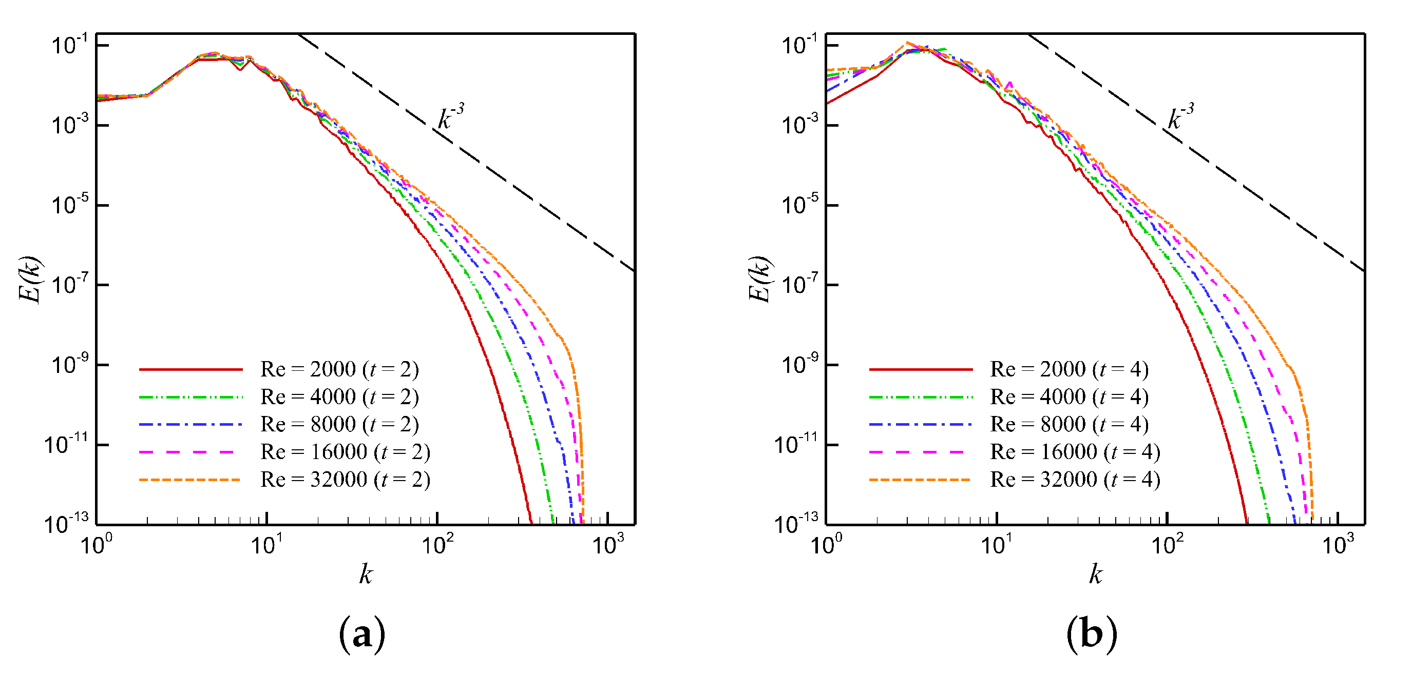
Figure 1. Evolution of energy spectra in 2D decaying Kraichnan turbulence for Re {2000, 4000, 8000, 16,000, 32,000 } at t = 2 (a) and t = 4 (b). Notice the convergence of energy spectrum in the inertial range to the k 3 scaling with increasing Reynolds number.
Fluids 05 00026 g001
Figure 2. A mesh independence test for Re = 16,000 (a) and Re = 32,000 (b) using two spatial resolutions. An acceptable match is obtained from both resolutions.
Fluids 05 00026 g002
Figure 3. Energy spectra obtained from partitioned ROM with P = 1 (a,b), P = 4 (c,d), and P = 8 (e,f). Note that P = 1 corresponds to the standard Galerkin-based reduced order model (ROM) with global proper orthogonal decomposition (POD) modes.
Fluids 05 00026 g003
Figure 4. Temporal evolution of the first and eighth modal coefficients using different numbers of partitions, compared to the true values obtained from the projection of FOM vorticity field on the corresponding basis function. (a) shows the first modal coefficient with P = 1 , while the eighth is given in (b). Results for P = 4 are shown in (c,d), while those for P = 8 are given in (e,f).
Fluids 05 00026 g004
Figure 5. Predicted results at time t = 4 showing vorticity contours in color with the level of streamfunction as height. (a) Full order model (FOM), (b) ROM ( R = 16 ) with P = 1 , (c) ROM ( R = 24 ) with P = 1 , and (d) ROM ( R = 32 ) with P = 1 . Note that P = 1 refers to the standard Galerkin ROM approach using a single partitioning zone.
Fluids 05 00026 g005
Figure 6. Predicted results at time t = 4 showing vorticity contours in color with the level of streamfunction as height. (a) Full order model (FOM), (b) ROM ( R = 16 ) with P = 1 , (c) ROM ( R = 16 ) with P = 4 , and (d) ROM ( R = 16 ) with P = 8 .
Fluids 05 00026 g006
Figure 7. Relative information content (RIC) of the snapshot matrix. (a) varying the number of partitions P, and (b) its sensitivity with respect to different zones for P = 4 case.
Fluids 05 00026 g007
Figure 8. Close-up views of temporal coefficients at the interfaces for P = 4 case.
Fluids 05 00026 g008
Figure 9. Temporal evolution of the first (a) and eighth (b) modal coefficients in the presence of closure modeling.
Fluids 05 00026 g009
Figure 10. Predicted results in the presence of closure modeling at time t = 4 showing vorticity contours in color with the level of streamfunction as height. (a) full order model (FOM), (b) ROM with κ = 0 , (c) ROM with κ = 4 , and (d) ROM with κ = 8 . For (bd): R = 16 and P = 1 .
Fluids 05 00026 g010
Figure 11. Energy spectra at final time predicted by ROMs in the presence of stabilization, compared to the FOM spectrum and k 3 scaling (a), with a compensated view in (b).
Fluids 05 00026 g011
Table 1. Root-mean-squares error at time t = 4 between Galerkin ROM (without any additional stabilization κ = 0 ) and FOM at Re = 16,000.
Model | | ψ R O M ψ F O M | | | | ω R O M ω F O M | |
P = 8 ( R = 16 ) 7.47 × 10 3 1.2774
P = 1 ( R = 16 ) 1.14 × 10 1 9.7322
P = 1 ( R = 24 ) 7.43 × 10 2 8.8779
P = 1 ( R = 32 ) 4.48 × 10 2 7.6098
P = 1 ( R = 48 ) 1.77 × 10 2 5.2468
P = 1 ( R = 64 ) 1.12 × 10 2 4.1695
P = 1 ( R = 96 ) 5.99 × 10 3 2.7428
P = 1 ( R = 128 ) 3.86 × 10 3 1.9213
Table 2. Root-mean-squares error at time t = 4 between the standard Galerkin ROM ( P = 1 , R = 16 ) and FOM in order to demonstrate the sensitivity with respect to the additional stabilization through κ at Re = 16,000.
Model with 16 Modes (P = 1) | | ψ R O M ψ F O M | | | | ω r o m ω F O M | |
κ = 0 1.14 × 10 1 9.7322
κ = 0.1 1.11 × 10 1 9.6010
κ = 0.25 1.07 × 10 1 9.4103
κ = 1.0 8.97 × 10 2 8.5579
κ = 2.0 7.24 × 10 2 7.6032
κ = 4.0 5.39 × 10 2 6.3506
κ = 8.0 5.27 × 10 2 5.6756
κ = 16.0 6.41 × 10 2 5.7574
Table 3. Root-mean-squares error at time t = 4 between the partitioned ROM ( P = 8 , R = 16 ) and FOM in order to demonstrate the sensitivity with respect to the additional stabilization through κ at Re = 16,000.
Model with 16 Modes ( P = 8 ) | | ψ R O M ψ F O M | | | | ω R O M ω F O M | |
κ = 0 7.47 × 10 3 1.2774
κ = 0.1 7.62 × 10 3 1.2627
κ = 0.25 7.85 × 10 3 1.2445
κ = 1.0 8.89 × 10 3 1.2058
κ = 2.0 1.01 × 10 2 1.2322
κ = 4.0 1.18 × 10 2 1.3574
κ = 8.0 1.40 × 10 2 1.5752
κ = 16.0 1.61 × 10 2 1.8108
Table 4. CPU time (in seconds) for ROM prediction and predetermined model coefficients computations, denoted as online and offline stages, respectively. We note that the CPU time assessments documented in this table are based on Fortran executions.
R = 16 R = 24 R = 32
P = 1
online 0.3889 1.1448 2.6925
offline 153.1237 393.5841 745.8216
P = 4
online 0.3719 1.1568 2.6026
offline 619.4428 1507.8947 3032.1081
P = 8
online 0.3699 1.1368 2.6036
offline 1142.9432 2882.4478 5776.0589