Changes in Vertical Distribution of Zooplankton under Wind-Induced Turbulence: A 36-Year Record

Atmosphere and Ocean Research Institute, The University of Tokyo, Kashiwa, Chiba 277-8564, Japan
Fluids 2019, 4(4), 195; https://doi.org/10.3390/fluids4040195
Submission received: 17 October 2019
/
Revised: 20 November 2019
/
Accepted: 22 November 2019
/
Published: 25 November 2019
(This article belongs to the Special Issue Fluid Mechanics of Plankton)
Abstract
:A multidecadal record of a local zooplankton community, stored in an open-access database, was analyzed with wind data to examine the impact of wind-induced turbulence on vertical distribution of zooplankton. Two major findings were made. First, the abundance of zooplankton assemblage (composed of copepods, cladocerans, etc.) in the upper layer (<10 m deep) decreased with increasing turbulence intensity, suggesting turbulence avoidance by zooplankton. Second, when focusing on each species, it was found that ambush (sit-and-wait) feeders showed statistically significant changes in response to turbulence, whereas suspension (filter) feeders did not. This is the first clear evidence that ambush feeders change vertical distribution in response to turbulence.
1. Introduction
While sub-centimeter-sized zooplankton play important roles in the marine ecosystem [1], processes that control their spatial distribution are elusive. Microscale turbulence, a ubiquitous characteristic of the ocean environment [2], significantly affects zooplankton swimming, feeding, and escape behavior [3]. Encounter rates with prey and mates are enhanced by environmental turbulence [4], but, at the same time, turbulence obscures signs of approaching predators, increasing the risks posed by staying in highly turbulent regions [5]. A numerical physical–ecological simulation, which considered the trade-off between reproduction and predation, suggested that avoidance of high levels of turbulence is most advantageous for reproduction [6]. Indeed, turbulence avoidance by zooplankton has been observed in small tank experiments, in which turbulence intensity was controlled by an oscillating grid [7]. However, field studies that demonstrate turbulence avoidance by zooplankton are limited [8,9,10,11]. Moreover, their conclusions are based on relatively short-term campaigns (<10 days) [8,9,10,11]. In this study, the impact of turbulence on zooplankton distribution was examined using a multidecadal record of a local zooplankton community and long-term sea-surface wind data.
2. Materials and Methods
2.1. Biological Parameters
Zooplankton data were obtained from an open-access database provided by the National Centers for Environmental Information. A biological dataset “36-Year Time Series (1963–1998) of Zooplankton, Temperature, and Salinity in the White Sea” [12] was used in this study. Zooplankton assemblage was sampled at the White Sea Biological Station (66°19.5′ N, 33°39.4′ E; the Arctic Ocean) from 1963 to 1998, i.e., 36 years. The water depth was 65 m at the station. A standard juday net was vertically towed every 10 days, collecting samples from surface (0 to 10 m deep), middle (10 to 25 m), and deep (25 to 65 m) layers. Mesh size and mouth area were 168 µm and 0.1 m2, respectively. Zooplankton were fixed with 10% formaldehyde solution and classified to the species level. The net tows were performed during daytime. A total of 814 net tows were made.
Representative vertical position, mean depth distribution (MDD; m) was calculated for each net tow:
where is the total abundance of zooplankton in the water column, is the abundance in the ith depth bin (i.e., i = 1, 2, and 3), and is the average depth of the ith depth bin (i.e., = 5 m, = 17.5 m, and = 45 m). MDD was calculated for the entire zooplankton assemblage, as well as for each species. In case a certain species was not observed in any depth layer, MDD was not calculated for this species. MDD and zooplankton abundance in the surface layer (individuals m−2) were analyzed with turbulence intensity.
2.2. Physical Parameters
Turbulence intensity at the biological station was estimated with wind data provided by the European Centre for Medium-Range Weather Forecasts. The historical reanalysis dataset “ERA-40” [13] was used in this study, covering the entire period of the biological data. A sequence of wind speed at 10 m above the sea surface at the biological station was downloaded with a temporal resolution of 6 h. Wind events may need to be sustained for several hours to affect underwater distribution of zooplankton [8,9,10,11]. Hence, representative wind speeds (m s−1) during the net tows were obtained by averaging wind speeds at 09:00 and 15:00 in local time ( and , respectively). The wind speed, , was rejected when the difference between and exceeded half of . Consequently, 105 of 814 data points (about 13%) were rejected.
Turbulent kinetic energy (TKE) dissipation rate (W kg−1), which is a typical parameter to quantify turbulence intensity, was estimated by the “law of wall” method. This study employs an empirical equation valid for the layers shallower than 10 m deep, which was provided by MacKenzie and Leggett (1993) [14]:
where is the volume-based TKE dissipation rate (W m−3) and is the depth (m). The empirical coefficients were , , and , respectively [14]. As suggested by Equation (2), turbulence intensity due to wind greatly varies along the vertical coordinate. To determine the representative turbulence intensity for the surface layer (0 to 10 m), the values were averaged over the surface layer, i.e., . Then, the averaged (W m−3) was converted to (W kg−1) based on the typical seawater density of 1028 kg m−3 [2]. Since Equation (2) is not applicable for ice-covered periods (November to May), values were rejected for those periods (296 of 814 data points; 36%). Finally, 419 pairs of biological and physical parameters were analyzed.
2.3. Statistical Analyses
Long-term environmental changes, such as slow climate changes, could induce long-term trends both in the physical and biological parameters, resulting in spurious correlations between them [15]. Hence, such long-term trends were examined by linear regression models. Seasonal changes, which have the same problem, were also examined by analysis of variance (ANOVA) tests and autocorrelation analyses. The ANOVA tests were performed for the data divided into monthly intervals (i.e., June, July, August, September, and October), whereas the autocorrelation analyses were applied to monthly averaged data. As autocorrelation is applicable for equally spaced data points, the winter data (i.e., November to May), which were not used for any other analyses, were included in the autocorrelation analyses.
Then, potential effects of ε on surface abundance and MDD of the entire assemblage were examined by linear regression models and ANOVA tests. Logarithmic values of were used for the linear regression models. The ANOVA tests were performed for the data divided into 8 intervals of different turbulence levels, which were equally spaced in logarithmic scale. The relationships between vs. the surface abundance and MDD were also examined based on the datum averaged over each cycle (i.e., June to October) to eliminate potential bias due to seasonal changes. The effects of on each zooplankton species were examined by two-sample t-tests, where the data were divided into 2 levels of turbulence: one for low (ε < 10−7 W kg−1) and the other for high (ε > 10−7 W kg−1).
3. Results
Wind speed reached 10 m s−1 during the analysis period. TKE dissipation rate, , ranged from 10−8 to 10−6 W kg−1. The average was = 2 × 10⁻⁷ ± 2 × 10⁻⁷ W kg−1 (mean ± standard deviation), typical in the surface layer [2]. Zooplankton assemblage was dominated by copepod species (Table 1), typical in the White Sea [16]. Abundance of entire zooplankton assemblage was highly concentrated in the surface layer (37,000 ± 46,000 individuals m−2) relative to the middle and deep layers (17,000 ± 23,000 and 5000 ± 10,000 individuals m–2, respectively). Average MDD of the entire assemblage was 12.9 ± 5.2 m.
Linear regression models showed that long-term trends were not statistically significant in ε (p = 0.639), surface abundance of entire assemblage (p = 0.324), nor MDD of the entire assemblage (p = 0.822) (Table 2). Yearly change in was −4 × 10⁻¹⁰ W kg−1 yr−1, which corresponds to an overall decrease of 10−8 W kg−1 for 36 years (Figure 1a). This is one order smaller than the standard deviation of . Similarly, overall changes were calculated as +7380 individuals m−2 for the surface abundance and −0.2 m for the MDD (Figure 1b,c), much smaller than the standard deviations of those parameters. In contrast, the ANOVA tests showed that seasonal trends were significant for the surface abundance (p < 0.001) and the MDD (p < 0.001) (Table 3). The surface abundance has a peak in August, while the MDD increased from early summer to fall (Figure 2b,c). Such seasonal cycles are also suggested by the autocorrelation analyses (Figure 3b,c). Seasonal cycles in were found in the autocorrelation analysis (Figure 3a) but not in the ANOVA test (p = 0.073; Table 3; Figure 2a).
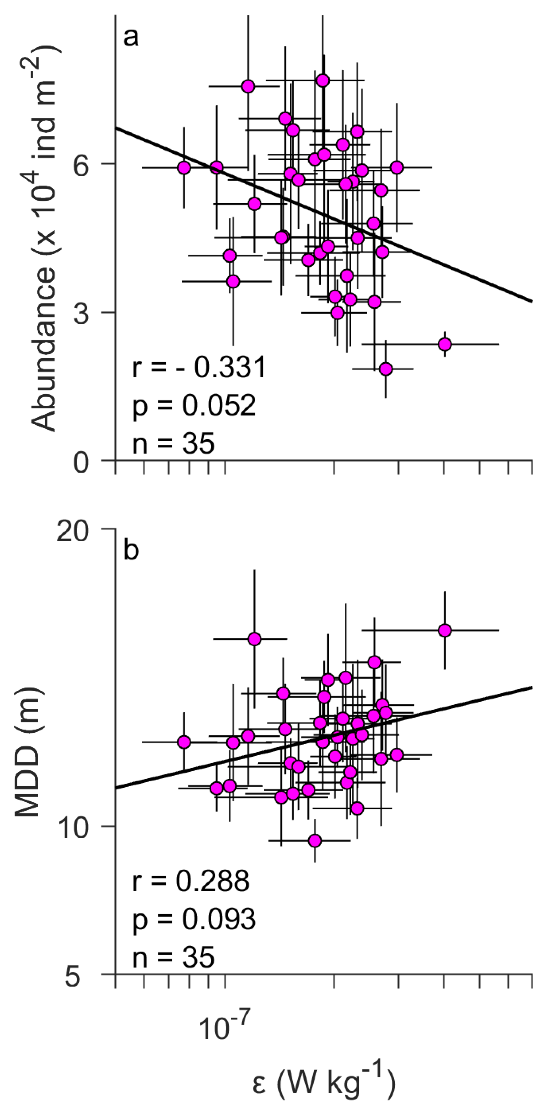
The surface abundance of the entire assemblage decreased with increasing (Figure 4a). The linear regression model shows a correlation coefficient of r = −0.12 (p = 0.012) between the surface abundance and (Table 4). Additionally, the MDD increased (deepened) with increasing (Figure 4c). The regression model shows r = 0.14 (p = 0.003; Table 4) for the MDD. Such trends against can be clearly seen in bar graphs (Figure 4b,d). The ANOVA tests showed statistically significant differences among the different levels of (p = 0.004 for the surface abundance and p = 0.010 for the MDD; Table 4). The analyses for the data averaged over seasonal cycles also suggested negative and positive slopes for the surface abundance (r = −0.33) and the MDD (r = 0.29), respectively (Figure 5), consistent with those for the raw data (Figure 4a,c). However, those trends were not statistically significant (p = 0.052 for the surface abundance and p = 0.093 for the MDD; Figure 5). This is probably due to the small range of the average (Figure 5).
When focusing on each species, the feeding mode was found to be associated with sensitivity to turbulence. Ambush feeders, such as calanoid copepod Oithona similis and chaetognath Saggita elegans, showed a statistically significant decrease in surface abundance and increase in the MDD in response to increased (p < 0.02; Table 1). In contrast, suspension feeders, such as calanoid copepod Temora longicornis, cladoceran Evadne nordmanni, and appendicularian Fritillaria borealis, showed no significant changes in surface abundance or MDD (Table 1). Calanoid copepod Acartia longiremis, which can switch between ambush and suspension feeding, exhibited no significant changes (Table 1). No changes were found for harpacticoid copepod Microstella norvegica, a particle feeder.
4. Discussion
Analysis of a multidecadal record of a local zooplankton community revealed avoidance of wind-induced turbulence by zooplankton, whereas significant response to turbulence was found only in ambush feeders (Table 1). This is consistent with laboratory experiments that demonstrated that ambush feeding is hindered by high levels of turbulence, while suspension feeding is less dependent on turbulence intensity [20,21]. Such turbulent effects on ambush feeding are also demonstrated by a theoretical model, which is designed to predict gut contents of ambush feeders in turbulent water [22]. In the literature, the model results were compared with those from field campaigns and showed that gut contents of ambush feeders decreased with increasing turbulence intensity [22]. Results from this study are consistent with those from the experimental and theoretical works [20,21,22].
In contrast to ambush feeders, pure suspension feeders exhibited no significant changes in response to turbulence. Given that suspension feeders are able to adapt to relatively high levels of turbulence [6], they probably place less priority on changing their position. Additionally, Acartia longiremis, which have multiple feeding modes, may switch their feeding mode to suspension feeding when in turbulent waters, rather than seek out low levels of turbulence (a similar discussion is seen in [21]). Although the particle feeder Microstella norvegica showed no significant changes in response to turbulence, this species, in another study, exhibited significant migration to deeper depths in response to wind-induced turbulence [11]. The reason for the difference between this study and the literature [11] remains unclear.
Physical processes, such as wind [23] and surface cooling [24], frequently disturb surface waters, producing vertical gradients in turbulence intensity in the water column [25]. Hence, downward migration is generally optimal behavior to seek lower levels of turbulence. However, turbulence is also generated by other processes, such as bottom stress associated with barotropic tides and swells [26], and shear stress associated with internal gravity waves [27]. Hence, actual turbulence intensities in the ocean would be different from those estimated by the simple model in Equation (2). This will result in errors in estimation of TKE dissipation rate (ε). Additionally, the reanalysis dataset would include potential errors in wind speed, which consequently induce additional errors in ε The European Centre for Medium-Range Weather Forecasts does not quantify the magnitude of the errors, but it could be substantial.
The r value of surface abundance vs. was r = −0.12 (Table 4), which corresponds to the coefficient of determination, r2, of 0.0144. This means only 1% of the fluctuation is explained by ε. Zooplankton generally exhibit highly intermittent distributions in the ocean, resulting in high levels of inter-sample variability in zooplankton density [28]. This means that single/instantaneous samples could have substantial (generally large) differences from the true density [28]. Such an inter-sample variability would be a source of potential errors (or biological noise) in surface abundance (Figure 1b, Figure 2b and Figure 4a).
Here, I compare turbulent velocity to typical swimming speeds of zooplankton. While turbulent flow speeds are highly variable in space and time, the representative velocity scale near the boundary is the friction velocity (m s−1). The friction velocity is a function of and the depth ( (m) (e.g., Equation (4.9) in [2]):
where is the von Karman constant (=0.41). Assuming ε = 10−7 W kg−1 (at which the significant changes in surface abundance and MDD were found) and = 10 m, we obtain = 0.7 cm s−1, which is on the same order as the turbulent velocity scales in the seasonal thermocline [29]. This is comparable with typical swimming speeds of sub-centimeter-sized zooplankton, but much lower than their instantaneous escape jumps >10 cm s−1 [29,30]. Hence, I suspect that they can perform oriented swimming even in highly turbulent waters to seek optimal levels of turbulence.
Despite the potential errors inherent in the open-access database, statistically significant trends were found between turbulence and ambush feeders. Turbulence estimation based on wind speed is valid for the surface layer and provides information about physical processes at scales of individual plankton, which is generally absent in biological samplings. I hope this study encourages other researchers to examine the reproducibility of the observed trends.
Funding
This research received no external funding.
Acknowledgments
The author gratefully acknowledges discussions with Amatzia Genin, Rubens M. Lopes, Gregory N. Ivey, Yoshinari Endo, J. Rudi Strickler, and Hidekatsu Yamazaki.
Conflicts of Interest
The author declares no conflicts of interest.
References
- Steinberg, D.K.; Landry, M.R. Zooplankton and the ocean carbon cycle. Annu. Rev. Mar. Sci. 2017, 9, 413–444. [Google Scholar] [CrossRef] [PubMed]
- Thorpe, S.A. The Turbulent Ocean; Cambridge University Press: Cambridge, UK, 2005. [Google Scholar]
- Kiørboe, T. A Mechanistic Approach to Plankton Ecology; Princeton University Press: Princeton, NJ, USA, 2008. [Google Scholar]
- Yamazaki, H.; Osborn, T.R.; Squires, K.D. Direct numerical simulation of planktonic contact in turbulent flow. J. Plankton Res. 1991, 13, 629–643. [Google Scholar] [CrossRef]
- Gilbert, O.M.; Buskey, E.J. Turbulence decreases the hydrodynamic predator sensing ability of the calanoid copepod Acartia tonsa. J. Plankton Res. 2005, 27, 1067–1071. [Google Scholar] [CrossRef]
- Visser, A.W.; Mariani, P.; Pigolotti, S. Swimming in turbulence: Zooplankton fitness in terms of foraging efficiency and predation risk. J. Plankton Res. 2009, 31, 121–133. [Google Scholar] [CrossRef]
- Seuront, L.; Yamazaki, H.; Souissi, S. Hydrodynamic disturbance and zooplankton swimming behavior. Zool. Stud. 2004, 43, 376–387. [Google Scholar]
- Lagadeuc, Y.; Boulé, M.; Dodson, J.J. Effect of vertical mixing on the vertical distribution of copepods in coastal waters. J. Plankton Res. 1997, 19, 1183–1204. [Google Scholar] [CrossRef]
- Incze, L.S.; Hebert, D.; Wolff, N.; Oakey, N.; Dye, D. Changes in copepod distributions associated with increased turbulence from wind stress. Mar. Ecol. Prog. Ser. 2001, 213, 229–240. [Google Scholar] [CrossRef]
- Visser, A.W.; Saito, H.; Saiz, E.; Kiørboe, T. Observations of copepod feeding and vertical distribution under natural turbulent conditions in the North Sea. Mar. Biol. 2001, 138, 1011–1019. [Google Scholar] [CrossRef]
- Maar, M.; Visser, A.W.; Nielsen, T.G.; Stips, A.; Saito, H. Turbulence and feeding behaviour affect the vertical distributions of Oithona similis and Microsetella norwegica. Mar. Ecol. Prog. Ser. 2006, 313, 157–172. [Google Scholar] [CrossRef]
- 36-Year Time Series (1963–1998) of Zooplankton, Temperature, and Salinity in the White Sea. Available online: https://www.nodc.noaa.gov/OC5/WH_SEA/index1.html (accessed on 20 November 2019).
- The ERA-40 archive. Available online: https://www.ecmwf.int/node/10595 (accessed on 20 November 2019).
- MacKenzie, B.R.; Leggett, W.C. Wind-based models for estimating the dissipation rates of turbulent energy in aquatic environments: Empirical comparisons. Mar. Ecol. Prog. Ser. 1993, 94, 207–216. [Google Scholar] [CrossRef]
- Prairie, Y.T.; Bird, D.F. Some misconceptions about the spurious correlation problem in the ecological literature. Oecologia 1989, 81, 285–288. [Google Scholar] [CrossRef] [PubMed]
- Pertsova, N.M.; Kosobokova, K.N. Zooplankton of the White Sea: Features of the composition and structure, seasonal dynamics, and the contribution to the formation of matter fluxes. Oceanol. C/C Okeanol. 2003, 43, S108–S122. [Google Scholar]
- Flood, P.R. House formation and feeding behaviour of Fritillaria borealis (Appendicularia: Tunicata). Mar. Biol. 2003, 143, 467–475. [Google Scholar] [CrossRef]
- Tönnesson, K.; Tiselius, P. Diet of the chaetognaths Sagitta setosa and S. elegans in relation to prey abundance and vertical distribution. Mar. Ecol. Prog. Ser. 2005, 289, 177–190. [Google Scholar] [CrossRef]
- Brun, P.; Payne, M.R.; Kiørboe, T. A trait database for marine copepods. Earth Syst. Sci. Data 2017, 9, 99–113. [Google Scholar] [CrossRef]
- Saiz, E.; Kiørboe, T. Predatory and suspension feeding of the copepod Acartia tonsa in turbulent environments. Mar. Ecol. Prog. Ser. 1995, 122, 147–158. [Google Scholar] [CrossRef]
- Saiz, E.; Calbet, A.; Broglio, E. Effects of small-scale turbulence on copepods: The case of Oithona davisae. Limnol. Oceanogr. 2003, 48, 1304–1311. [Google Scholar] [CrossRef]
- Pécseli, H.L.; Trulsen, J.K.; Stiansen, J.E.; Sundby, S.; Fossum, P. Feeing of plankton in turbulent oceans and lakes. Limnol. Oceanogr. 2019, 64, 1034–1046. [Google Scholar] [CrossRef]
- Oakey, N.S.; Elliott, J.A. Dissipation within the surface mixed layer. J. Phys. Oceanogr. 1982, 12, 171–185. [Google Scholar] [CrossRef]
- Shay, T.J.; Gregg, M.C. Convectively driven turbulent mixing in the upper ocean. J. Phys. Oceanogr. 1986, 16, 1777–1798. [Google Scholar] [CrossRef]
- Smyth, W.D.; Moum, J.N. 3D Turbulence. In Encyclopedia of Ocean Sciences, 3rd ed.; Cochran, J.K., Bokuniewicz, H.J., Yager, P.L., Eds.; Elsevier Ltd.: London, UK, 2019; Volume 3, pp. 486–496. [Google Scholar]
- Drost, E.J.F.; Lowe, R.J.; Ivey, G.N.; Jones, N.L. Wave-current interactions in the continental shelf bottom boundary layer of the Australian North West Shelf during tropical cyclone conditions. Cont. Shelf Res. 2018, 165, 78–92. [Google Scholar] [CrossRef]
- Kokubu, Y.; Yamazaki, H.; Nagai, T.; Gross, E.S. Mixing observations at a constricted channel of a semi-closed estuary: Tokyo Bay. Cont. Shelf Res. 2013, 69, 1–16. [Google Scholar] [CrossRef]
- Downing, J.A.; Pérusse, M.; Frenette, Y. Effect of interreplicate variance on zooplankton sampling design and data analysis. Limnol. Oceanogr. 1987, 32, 673–680. [Google Scholar] [CrossRef]
- Yamazaki, H.; Squires, K.D. Comparison of oceanic turbulence and copepod swimming. Mar. Ecol. Prog. Ser. 1996, 144, 299–301. [Google Scholar] [CrossRef]
- Buskey, E.J.; Swift, E. Behavioral responses of oceanic zooplankton to simulated bioluminescence. Biol. Bull. 1985, 168, 263–275. [Google Scholar] [CrossRef]
Figure 1.
Time series for turbulent kinetic energy dissipation rate (a), surface abundance of the entire assemblage (0 to 10 m deep) (b), and mean depth distribution (MDD) of the entire assemblage (c). Filled circles denote raw data. Red lines denote linear regression models. Results of the regression models are summarized in Table 2.
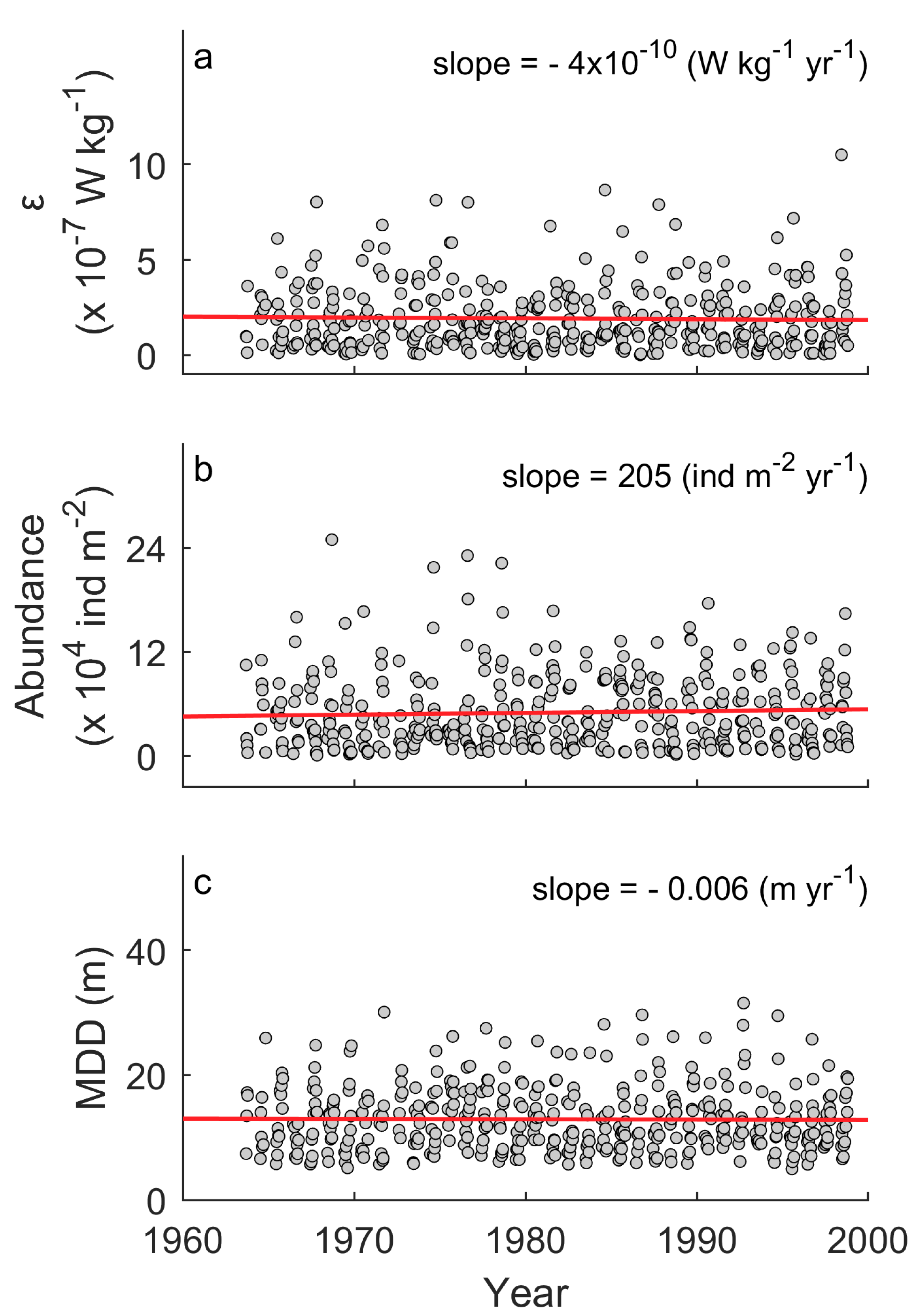
Figure 2.
Seasonal trends in turbulent kinetic energy dissipation rate (a), surface abundance of the entire assemblage (0 to 10 m deep) (b), and mean depth distribution (MDD) of the entire assemblage (c). Filled circles denote raw data. Horizontal bars denote averages over month categories (i.e., June, July, August, September, and October). Error bars denote standard error. Results of the ANOVA tests are summarized in Table 3.
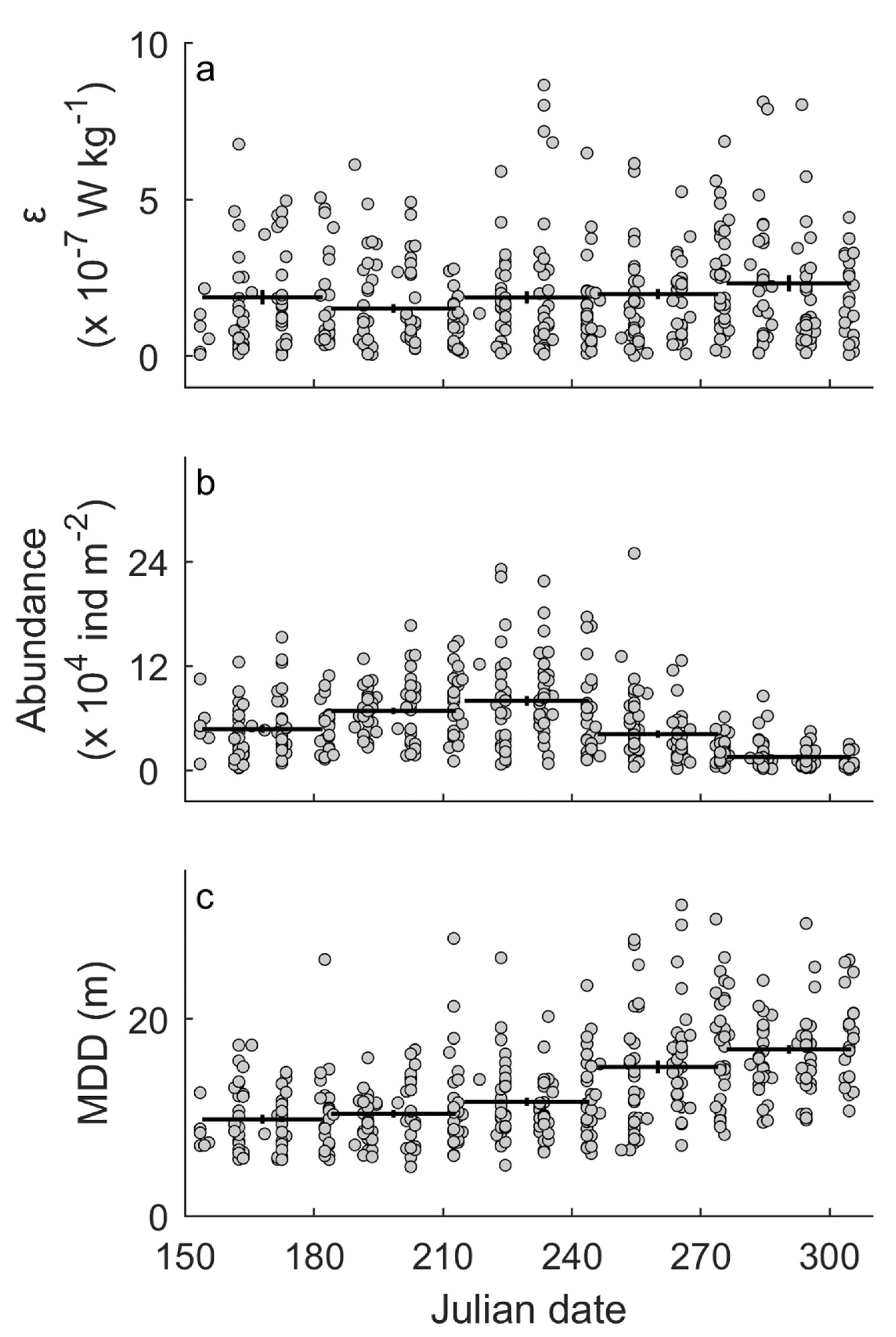
Figure 3.
Results from the autocorrelation analyses on turbulent kinetic energy dissipation rate (ε) (a), surface abundance of the entire assemblage (0 to 10 m deep) (b), and mean depth distribution (MDD) of the entire assemblage (c). Red lines denote 99% confidence intervals.
Figure 3.
Results from the autocorrelation analyses on turbulent kinetic energy dissipation rate (ε) (a), surface abundance of the entire assemblage (0 to 10 m deep) (b), and mean depth distribution (MDD) of the entire assemblage (c). Red lines denote 99% confidence intervals.

Figure 4.
Surface abundance (0 to 10 m deep) (a,b) and mean depth distribution (MDD) (c,d) of the entire assemblage vs. turbulent kinetic energy dissipation rate (ε). The panels on the left show raw data. Each circle corresponds to a vertical net tow sample (n = 419). Solid lines denote linear regression models. The panels on the right show averages for different levels of turbulence. Error bars denote standard error. Results of the linear regression models and ANOVA tests are summarized in Table 4.
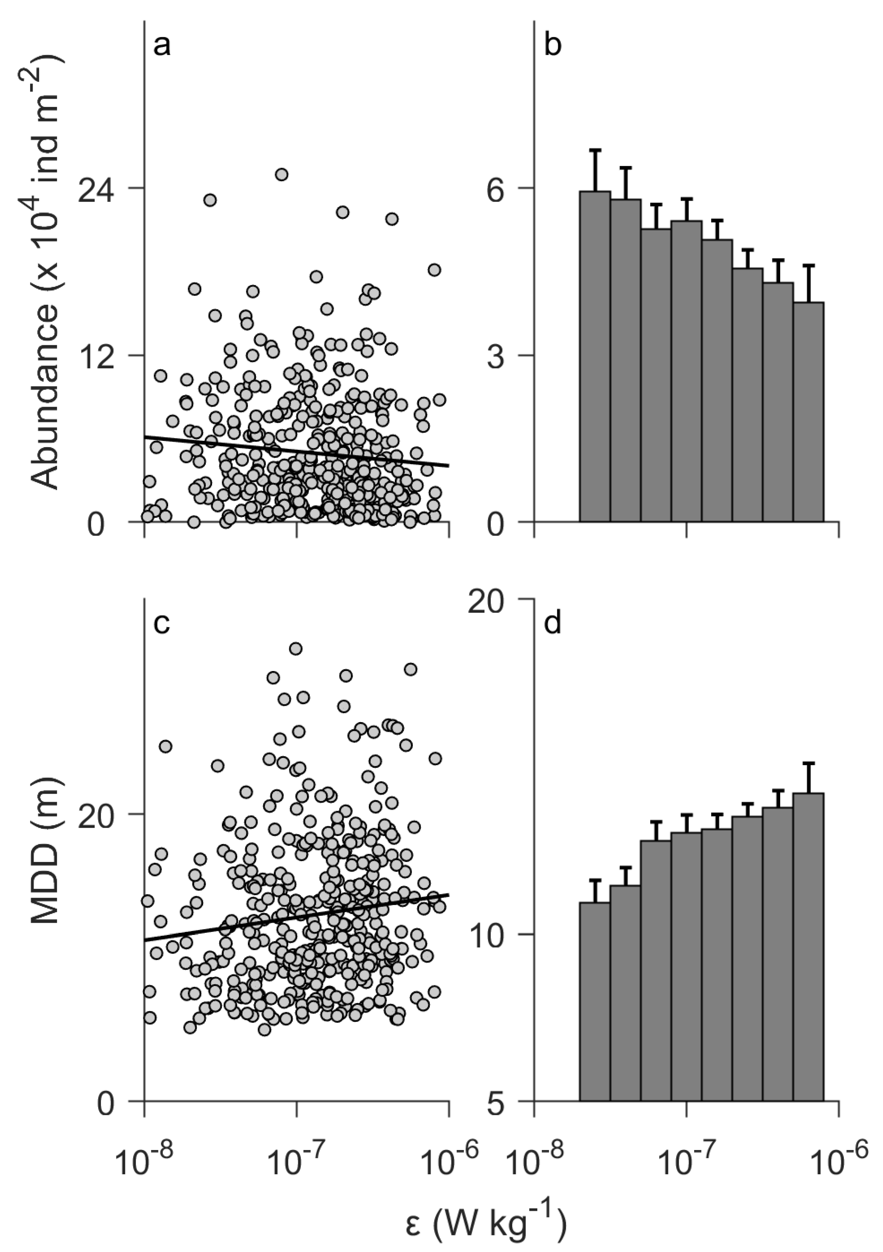
Figure 5.
Same figures as in Figure 4 (left panels) but for the data averaged over seasonal cycle (i.e., June to October). Horizontal and vertical lines denote standard error. The first year, 1963, was excluded since net tows started from September. The number of samples is n = 35.
Figure 5.
Same figures as in Figure 4 (left panels) but for the data averaged over seasonal cycle (i.e., June to October). Horizontal and vertical lines denote standard error. The first year, 1963, was excluded since net tows started from September. The number of samples is n = 35.

Table 1.
List of zooplankton species. Feeding mode definitions are based on the literature [17,18,19]. The effects of turbulence intensity on surface abundance (0 to 10 m deep) and mean depth distribution (MDD) were examined by two-sample t-tests, where the data were divided into two levels of turbulence: one for low ( < 10−7 W kg−1) and the other for high ( > 10−7 W kg−1). Boldface italics indicate statistical significance (p < 0.02).
| Surface Abundance (×103 ind m−2) | MDD (m) | |||||||||
|---|---|---|---|---|---|---|---|---|---|---|
| t-Test | t-Test | |||||||||
| Feeding Mode | Turbulence Level | Mean ± Standard Error | df | t-Value | p-Value | Mean ± Standard Error | df | t-Value | p-Value | |
| Copepod | ||||||||||
| Acartia longiremis | Ambush/suspension | Low | 3.13 ± 0.30 | 417 | 0.76 | 0.449 | 12.45 ± 0.58 | 405 | −0.50 | 0.619 |
| High | 2.87 ± 0.32 | 13.05 ± 0.60 | ||||||||
| Microstella norvegica | Particle | Low | 0.43 ± 0.10 | 417 | 1.06 | 0.290 | 13.47 ± 0.73 | 199 | −0.17 | 0.864 |
| High | 0.52 ± 0.11 | 13.17 ± 0.61 | ||||||||
| Oithona similis | Ambush | Low | 35.53 ± 2.19 | 417 | 3.50 | 0.001 | 11.98 ± 0.34 | 417 | −2.55 | 0.011 |
| High | 26.96 ± 1.96 | 13.10 ± 0.35 | ||||||||
| Temora longicornis | Suspension | Low | 7.36 ± 1.05 | 417 | −0.29 | 0.771 | 13.36 ± 0.59 | 378 | −1.99 | 0.047 |
| High | 6.86 ± 1.08 | 14.54 ± 0.55 | ||||||||
| Chaetognath | ||||||||||
| Saggita elegans | Ambush | Low | 0.53 ± 0.08 | 417 | 2.85 | 0.005 | 24.53 ± 0.85 | 401 | −2.54 | 0.011 |
| High | 0.42 ± 0.09 | 27.78 ± 0.84 | ||||||||
| Cladoceran | ||||||||||
| Evadne nordmanni | Suspension | Low | 4.35 ± 0.57 | 417 | 1.71 | 0.088 | 7.64 ± 0.40 | 353 | −0.97 | 0.335 |
| High | 2.98 ± 0.42 | 7.83 ± 0.33 | ||||||||
| Appendiclarian | ||||||||||
| Fritillaria borealis | Suspension | Low | 3.98 ± 0.55 | 417 | 1.42 | 0.156 | 9.68 ± 0.45 | 361 | −1.35 | 0.179 |
| High | 3.66 ± 0.83 | 10.66 ± 0.52 | ||||||||
Table 2.
Results of linear regression models to examine long-term trends in turbulent kinetic energy dissipation rate (denoted as “”), surface abundance of entire assemblage (0 to 10 m deep) (“Abundance”), and mean depth distribution of the entire assemblage (“MDD”). Data from Figure 1.
Table 2.
Results of linear regression models to examine long-term trends in turbulent kinetic energy dissipation rate (denoted as “”), surface abundance of entire assemblage (0 to 10 m deep) (“Abundance”), and mean depth distribution of the entire assemblage (“MDD”). Data from Figure 1.
| y = ax + b | ||||
|---|---|---|---|---|
| n | a | b | p-Value | |
| ε | 419 | −4 × 10⁻¹⁰ | 1 × 10⁻⁶ | 0.639 |
| Abundance | 419 | 205 | −4 × 10⁵ | 0.324 |
| MDD | 419 | −0.006 | 24 | 0.822 |
Table 3.
ANOVA table to examine the effects of month (denoted as “Month”) on turbulent kinetic energy dissipation rate (“”), surface abundance of entire assemblage (0 to 10 m deep) (“Abundance”), and mean depth distribution (“MDD”) of the entire assemblage. Data from Figure 2.
Table 3.
ANOVA table to examine the effects of month (denoted as “Month”) on turbulent kinetic energy dissipation rate (“”), surface abundance of entire assemblage (0 to 10 m deep) (“Abundance”), and mean depth distribution (“MDD”) of the entire assemblage. Data from Figure 2.
| Source | df | SS | MS | F | p-Value | |
|---|---|---|---|---|---|---|
| ε | Month | 4 | 3 × 10–13 | 8 × 10–14 | 2.2 | 0.073 |
| Abundance | Month | 4 | 2 × 10¹¹ | 6 × 10¹⁰ | 42.7 | <0.001 |
| MDD | Month | 4 | 3271 | 818 | 42.5 | <0.001 |
Table 4.
Results of linear regression models and ANOVA tests to examine the effects of turbulent kinetic energy dissipation rate (denoted as “ε”) on surface abundance of the entire assemblage (0 to 10 m deep) (“Abundance”) and mean depth distribution (“MDD”) of entire assemblage. r denotes the correlation coefficient. Data from Figure 4.
| Linear Regression Model | ANOVA | ||||||||||
|---|---|---|---|---|---|---|---|---|---|---|---|
| y = ax + b | |||||||||||
| n | a | b | r | p-Value | Source | df | SS | MS | F | p-Value | |
| Abundance | 419 | −1 × 10⁴ | 3 × 10⁴ | −0.12 | 0.012 | ε | 7 | 3 × 10¹⁰ | 4 × 10⁹ | 2.2 | 0.004 |
| MDD | 419 | 1.57 | 23.8 | 0.14 | 0.003 | ε | 7 | 510 | 73 | 2.7 | 0.010 |
© 2019 by the author. Licensee MDPI, Basel, Switzerland. This article is an open access article distributed under the terms and conditions of the Creative Commons Attribution (CC BY) license (http://creativecommons.org/licenses/by/4.0/).
Share and Cite
MDPI and ACS Style
Tanaka, M. Changes in Vertical Distribution of Zooplankton under Wind-Induced Turbulence: A 36-Year Record. Fluids 2019, 4, 195. https://doi.org/10.3390/fluids4040195
AMA Style
Tanaka M. Changes in Vertical Distribution of Zooplankton under Wind-Induced Turbulence: A 36-Year Record. Fluids. 2019; 4(4):195. https://doi.org/10.3390/fluids4040195
Chicago/Turabian StyleTanaka, Mamoru. 2019. "Changes in Vertical Distribution of Zooplankton under Wind-Induced Turbulence: A 36-Year Record" Fluids 4, no. 4: 195. https://doi.org/10.3390/fluids4040195