Molecular Dynamics Simulation of the Superspreading of Surfactant-Laden Droplets. A Review
by
 , , , and
Panagiotis E. Theodorakis
1,* ,
,
Edward R. Smith
2,*,
Richard V. Craster
3,*,
Erich A. Müller
4,* and
Omar K. Matar
4,* 1
Institute of Physics, Polish Academy of Sciences, Al. Lotników 32/46, 02-668 Warsaw, Poland
2
Department of Mechanical and Aerospace Engineering, Brunel University London, Uxbridge, Middlesex UB8 3PH, UK
3
Department of Mathematics, Imperial College London, Exhibition Road, South Kensington, London SW7 2AZ, UK
4
Department of Chemical Engineering, Imperial College London, Exhibition Road, South Kensington, London SW7 2AZ, UK
*
Authors to whom correspondence should be addressed.
Fluids 2019, 4(4), 176; https://doi.org/10.3390/fluids4040176
Submission received: 5 September 2019
/
Revised: 20 September 2019
/
Accepted: 27 September 2019
/
Published: 1 October 2019
(This article belongs to the Special Issue Coupled Flow and Heat or Mass Transport)
Abstract
:Superspreading is the rapid and complete spreading of surfactant-laden droplets on hydrophobic substrates. This phenomenon has been studied for many decades by experiment, theory, and simulation, but it has been only recently that molecular-level simulation has provided significant insights into the underlying mechanisms of superspreading thanks to the development of accurate force-fields and the increase of computational capabilities. Here, we review the main advances in this area that have surfaced from Molecular Dynamics simulation of all-atom and coarse-grained models highlighting and contrasting the main results and discussing various elements of the proposed mechanisms for superspreading. We anticipate that this review will stimulate further research on the interpretation of experimental results and the design of surfactants for applications requiring efficient spreading, such as coating technology.

1. Introduction
Superspreading is the unexpectedly fast and complete spreading (Figure 1) of surfactant-laden aqueous droplets on hydrophobic substrates, a phenomenon that has attracted significant attention over the last decades [1,2,3,4,5,6]. Surfactants that are responsible for this phenomenon are known as superspreaders with the most well-known example being Silwet-L77, which belongs to the family of trisiloxane surfactants. These surfactants have a characteristic hydrophobic head group composed of three siloxane chemical groups and a hydrophilic alkyl ether tail, which may vary in length or composition (Figure 2). Superspreading is important for many applications in a wide range of different areas, such as coating technology, drug and herbicides delivery, and enhanced oil recovery [3,7,8,9,10], manifested as enhanced fluid flow and efficient spreading. In view of the large spectrum of applications, superspreading has motivated a wide range of experimental [11,12,13,14,15,16,17,18], as well as numerical and simulation research in the recent years [19,20,21,22,23,24,25,26]. The main focus of these studies has been the underlying mechanisms of this phenomenon and identifying key features that distinguish superspreaders from other common (or conventional) surfactants. Due to these challenges, this research area continues to attract attention.
The manifestation of superspreading takes place at the macroscopic level [4], where the spreading of a droplet is much faster in the case of a droplet with superspreading surfactant than in the case of a droplet with a common surfactant (Figure 1). In the latter case, the radius of the droplet base increases as with the exponent (Tanner’s law) [27], while in the case of superspreading, exponents as large as have been reported in experiments [2,28] and simulations [20]. Another characteristic of superspreading behaviour is the dependence of the spreading rate and the droplet contact-angle on surfactant concentration. Both properties do not vary monotonically with the increase of surfactant concentration, but both initially increase with surfactant concentration and then decrease upon further increase of the concentration [2,20]. Experiments have carefully studied the effect of various factors on spreading as exeplified by studies on the rate of evaporation [29], humidity [30], pH [31], influence of surfactant structure and concentration [32,33], surfactant aging effects [34], the behaviour of surfactant mixtures [35,36], substrate hydrophobicity [2,30,37], and temperature [32,38]. Although these studies have provided a great deal of information, understanding the superspreading mechanism and the key design features of superspreaders remains elusive. This is due to the inability of experiment to capture the underlying microscopic processes that dictate the superspreading phenomenon. Moreover, varying conditions can often lead to contradictory results between different experiments [5].
Another way of studying superspreading is with numerical simulation [23,24,25]. For example, Karapetsas et al. have studied the superspreading of surfactant-laden droplets by using continuum simulation based on lubrication theory, advection–diffusion equations and chemical kinetic fluxes for the surfactant transport [25]. Based on a system of coupled equations, the numerical model obtained results for the droplet thickness, interfacial concentrations of surfactant monomers, and bulk concentrations of monomers and aggregates. Thus, the various adsorption processes within the droplet and aggregation properties of the surfactant were properly taken into consideration. This model highlights the adsorption of surfactant from the liquid–vapour (LV) surface at the substrate through the contact line (CL) as an indispensable part of the superspreading mechanism. The authors have also underlined the role of high Marangoni stresses close to the droplet edge due to the surfactant depletion at the LV surface as a driving force for the fast spreading. The Karapetsas et al. [25] model predicted values of spreading exponents or even higher, while the non-monotonic variation of the spreading rate with surfactant concentration was captured by the model in agreement with experimental observations [2]. Recently, computational fluid dynamics and theoretical models [23] have been employed to study superspreading confirming these predictions [24]. While numerical simulation and theory have contributed significantly to unveiling the superspreading mechanism, both are unable to describe the microscopic behaviour of the systems. In these models, the microscopic effects (for example, the contact angle, slip, the liquid-vapour interface, etc.) are model assumptions that have to be incorporated in the equations through empirical coefficients.
In contrast to continuum modelling and analytical theory, molecular simulation does not face such issues and can capture the microscopic behaviour of the system in detail. Molecular-level methods can track molecules at any time under controlled conditions during the in silico experiment. Nowadays, the existence of reliable force-fields for water–surfactant systems based on all-atom [39,40,41,42] and coarse-grained (CG) models [43,44,45,46,47,48,49,50,51,52,53,54,55,56,57,58,59,60] enable the genuine simulation of such systems. For example, recent simulations of aqueous solutions with surfactants [21,22,61,62,63,64,65,66,67] have established the connection between the behaviour of surfactants in the bulk and spreading [68,69,70,71], while the superspreading mechanism and the main characteristics of superspreading surfactants have been the focus of recent studies [5,19,20,21,22,23,24,68,70,71,72]. In view of these important advances in the superspreading arena, this review will highlight what we believe are the most important methods and results obtained by molecular dynamics (MD) simulation of all-atom and CG models. Hence, our discussion will evolve as follows: In Section 2, we will describe various all-atom and CG methods that have been so far employed to investigate superspreading. In Section 3, we will present relevant results obtained by MD simulation based on these models. Finally, in Section 4, we will briefly discuss future perspectives in the research area of superspreading.
2. Methods
2.1. All-Atom Models
There are a number of all-atom models (Figure 2), which can be applied in the case of water–surfactant systems. Still, these models require testing in order to confirm that key properties of the system are well reproduced. Such properties may include the phase behaviour of the water–surfactant system, surface tension, and dynamic properties such as diffusion, adsorption coefficients, etc. The number of all-atom studies on the superspreading is small, since these simulations are computationally demanding posing severe restrictions on the size of the system and the interpretation of the simulation results may be limited in scope. However, all-atom force-fields generally perform well since they are obtained from high-resolution data, for example quantum mechanics calculations. An example of a popular all-atom force-field is AMBER, which is widely used for the simulation of proteins [73], but it can also be applied in the case of water–surfactant systems. To this end, Nikolov et al. have used the AMBER force-field to study the conformations of Silwet-L77 and n-octyl-phenyl-polyglycol(10)-ether (OP10EO) at the water surface [74]. The high computational cost of this all-atom model would only allow, at that time, for 1 ns trajectories for an ensemble of 50 configurations. It was found that the adsorbed trisiloxane hydrophobe is much more compact and occupies less space than the elongated OP10EO molecule. Moreover, a higher spreading pressure in the case of the Silwet-L77 surfactant was observed [74].
Halverson et al. [70,75] has studied the wetting of graphite by considering cylindrical and spherical water and surfactant-laden aqueous droplets by all-atom simulation. In this model, droplets comprised of about 10,000 molecules were considered, which corresponds to a radius of 4 nm. The number of surfactant molecules (C12E4 or M(D’E4OH)M) is of the order of 400 on the surface of the droplet considering also the addition of another 98 molecules in order to account for a large concentration of molecules at the interfaces during spreading. In this case, the SPC/E model for water was employed [76], while for the interaction with the graphite substrate, the Lennard–Jones (LJ) potential was used with the graphite atoms being fixed at their positions as suggested by Werder et al. [59]. For modelling the surfactants, Halverson et al. have used the OPLS-UA force-field [77,78] and a force field for polydimethylsiloxane [79] through the OPLS combining rules. In principle, one can combine generic models with a tailor-made dimethylsiloxane model, for example, the model of Sun et al. [80] or the model of Frischknecht et al. [81]. Moreover, as is usually done for organic molecules in all-atom force-fields, the 1–4 pair interactions (non-bonded interactions for atoms separated by three or fewer bonds, e.g., LJ) were excluded. The cutoff of the short-range interaction was set to 10 Å and the timestep was 2 fs. Halverson et al. have also considered the wetting of methyl-and hydroxyl-terminated SAMs by neat, or nearly water-free, trisiloxane droplets with results acquired at room and at a high temperature (450 K) [70].
The above models are based on the direct use of the force-field parameters without any refinement of the parameters to simulate water–surfactant systems. In a more recent study by all-atom models, Isele-Holder et al. [21,22] have obtained atomistic potentials for trisiloxane, alkyl ethoxylate and perfluoroalkane-based surfactants that are compatible with the TIP4P/2005 model for water [82]. The surface tension of the systems was in agreement with experiment [83]. In contrast, other common water models, such as TIP3P, TIP4P [84], and SPC/E [76] tend to underestimate the surface tension of water [83]. To build the model for trisiloxane, one may use building blocks from well-known force-fields, such as OPLS [85], GROMOS [86], CHARMM [87], AMBER [88], and TraPPE [89]. However, these force-fields may not be compatible with the TIP4P/2005 water model and typically do not contain parameters for dimethylsiloxane. A way forward may be to use the force-fields of Sun et al. [80] or Frischknecht et al. [81], but these models may still not be compatible with the TIP4P/2005 water model. Hence, Isele-Holder et al. have chosen instead to use models for polyalkenes [90], poly(ethylene oxide) [91], poly(tetrafluoroethylene) [92], and poly(dimethylsiloxane) [93], which were obtained by quantum chemistry calculations without empirical fits and thus they can be considered as transferable. Isele-Holder et al. also pointed out the importance of including the long-range dispersion forces and ensuring that all force-field parameters, including parameters of the original force field, follow geometric combining rules [94], which is also a computationally efficient approach. Finally, they have ensured that the models are compatible with the TIP4P/2005 water model and that any missing bonded interactions or partial charges due to building surfactants from the above different polymers are parameterised [21]. For all-atom models and the following CG models, standard NVT simulations have been used to study the water–surfactant systems.
2.2. Bead–Spring Models
A simple bead–spring model can capture the properties of complex systems, including water–surfactant systems. An example of such a model in the context of superspreading has been proposed by Tomassone et al. (Figure 3) [61,62,68]. This model has been also used by Kim et al. [69] in their studies. The model dates back to 2001, when Tomassone et al. developed a CG model to study the gas-liquid phase transitions of soluble and insoluble surfactants at a fluid interface with MD simulation. This model assumes LJ interactions between different components, whose strength, , is
Here, r is the distance between any two beads, relates to the size of the spherical beads, and expresses the strength of interaction. In this model, the repulsive interaction is the same, irrespective of the bead type, while the attractive interaction between beads is fine-tuned by changing the parameter , in this way accounting for different particle types that correspond to the hydrophilic head of a surfactant molecule (type 1), the hydrophobic tail (type 2), the solvent (type 3), and the solid substrate (type 4). In the more recent work by Shen et al., these coefficients are chosen to account for strong (Case 1) and weaker (Case 2) interactions between the hydrophilic parts of the surfactants and the solvent [68]. The values of the coefficients in the case of Shen et al. are reported in Table 1. A different set of interactions has been considered in the work of Tomassone et al. [61,62] and Kim et al. [69]. This underlines the flexibility of these models in investigating different situations by tuning the relative strength of interactions between different components in water–surfactants systems. Linear and T-shaped surfactants are constructed by bonding beads by means of the finitely extensible nonlinear elastic (FENE) potential
where r is the distance between two consecutive beads along the surfactant chain, expresses the maximum extension of the bond, and is an elastic constant. In the case of the T-shaped surfactant, the three consecutive beads of the hydrophobe are kept linear by using a harmonic angle potential
where is the angle between three consecutive beads and . A force constant of was used, which is able to maintain the linear geometry of the hydrophobe in the T-shaped surfactant (Figure 3). This model does not attempt to provide a realistic molecular model for trisiloxane and linear chain surfactant molecules, but instead aims to imitate an analogous system on the basis of short-range LJ potential. Moreover, charges are neglected. However, the use of this kind of bead–spring CG models allows for the exploration of larger systems over longer simulation times than would be possible with any all-atom model. For this reason, CG models have been used recently to study superspreading. In the following, we will discuss two popular CG models, which take into account, in more detail, the characteristics of the CG groups of atoms. These have been employed in the study of surfactant–water systems in the context of superspreading, namely the MARTINI [60] and the Statistical Associating Fluid Theory (SAFT) [95] models.
2.3. MARTINI Model
The MARTINI model [60,96] has been employed to study linear and T-shaped surfactants with possible implications for superspreading (Figure 3). A significant advantage of the MARTINI force-field with respect to the above CG models, is the ability to take into account the chemical identity of CG groups of atoms. The ‘Lego’ approach adopted in the MARTINI model allows for the simulation of a wide spectrum of diverse molecules without the need to refine the force-field parameters. Hence, it offers practically an all-atom resolution while being computationally as cheap as a CG model [97]. This is due to the smaller number of interaction sites (fewer force calculations are required in the MD code), the simple functional forms of the interaction potentials with a small cutoff (e.g., LJ potential) and the additional speed-up that generally stems from the smoother energy landscape in the case of CG models. The latter combined with the slower modes of heavier CG beads allows a larger time step and consequently longer realistic simulation times.
The innovative ‘Lego’ approach that underpins the MARTINI force-field categorises atomic functional groups into four main categories depending on their charge and polarity as follows: polar, nonpolar, apolar, and charged. Each category is then subdivided into subcategories to refine further the interaction, resulting in ten basic levels on interaction in the original MARTINI model [97]. All chemical groups, irrespective of whether they are part of a lipid, a protein, a nucleic-acid chain or any other molecule, are built by beads that interact through this limited number of interactions. These interaction levels are constantly refined (the MARTINI version 3.0 was released in 2019) and new types of beads are also added in order to be able to simulate an ever broader range of different molecules. In the MARTINI model, nonbonded interactions are expressed through the LJ potential
where the strength of interaction between different functional groups and is tuned via the parameter according to the available MARTINI levels of interaction. The Coulombic potential is used for the electrostatic interactions considering an integer value of charge for the charged beads, that is
where is the total charge of the group (bead), is the permittivity in vacuum, and is the relative dielectric constant. In the standard MARTINI model, , or when the polarisable MARTINI water model is used. Bond and angle interactions are dealt with the standard harmonic potential functions. The MARTINI water model (the polarisable MARTINI water model has been particularly developed to prevent freezing) is based on a single bead that corresponds to four water molecules. The temperature is a control parameter in an NVT simulation based on the MARTINI model and it does not have any physical meaning. Finally, extensive information and a range of user tutorials, based on the GROMACS package [98], are provided by the developers and the MARTINI community [99,100], which renders this force-field easy to use in the MD simulation of a variety of systems.
2.4. Statistical Associating Fluid Theory Model
The SAFT CG force-field has been used for the study of water–surfactant systems [19,66,67,101,102,103] and particularly in the context of superspreading (Figure 4) [5,19,20,26,72]. This CG model is derived from the SAFT- molecular-based equation of state (EoS), which can describe analytically experimental data [104,105]. In practice, the EoS offers an accurate fit for the force-field parameters, where the key nonbonded interactions are expressed by means of the Mie potential (Equation (6)). The macroscopically observed thermophysical properties that stem from the fluid–fluid and fluid–solid interactions are well reproduced by the model, which is a direct consequence of the close match between the theory and the underlying Hamiltonian of the system [65,66,67,95,101,106,107,108,109]. The SAFT approach derives robust and transferable potentials of effective beads that represent groups of atoms as in the case of the MARTINI model. In the case of the SAFT- force-field, the force-field parameters of a particular functional group of atoms have to be derived by the theory and reproduce for each case the experimental data. For this reason, the SAFT CG model will always guarantee agreement with experiment (Figure 4). The approach can also describe heterogeneous chain fluids comprised by different functional groups [107]. The interaction parameters are traced to macroscopic properties of the original segments of the corresponding pure components [95].
In the case of water–surfactant systems with trisiloxane superspreading or common surfactants, a bead ‘W’ may represent two water molecules, while effective beads ‘M’ may correspond to a chemical group, effective beads ‘D’ to groups, ‘EO’ to (ether) chemical groups, and ‘CM’ to (alkane). By using these beads, one may model a wide range of different surfactants, which include both superspreading and nonsupersprading (common) surfactants (Figure 4) [26]. The model also takes also into account the different masses of the chemical beads. The values of these masses are presented in Table 2.
In the SAFT CG model, the interaction between non-bonded beads takes place through the Mie potential, which offers a greater flexibility in reproducing thermophysical properties of the system. The Mie potential reads
where
i and j indicate the bead type (e.g., W, M, etc.). expresses the size of the effective beads and the strength of interaction. and are parameters of the Mie potential, while is the distance between any two effective beads. The values of the Mie potential parameters for different pairs of beads are summarised in Table 3; A universal cutoff for all nonbonded interactions is set to . In addition, , irrespective of the bead type since this expresses the dispersion interactions between beads [112].
Beads are connected with harmonic potentials, expressed in mathematical form as follows:
where values of are given in Table 3, and . is the unit of length while is the energy unit. Moreover, EO effective beads along the chain interact via a harmonic angle potential of the form
where is the angle between beads i, j and k. /rad2 is a constant expressing the strength of the harmonic potential (stiffness of the chain), and rad is the equilibrium angle.
The above potentials define the SAFT model for the water and the surfactant. Two different approaches can be followed for modelling the substrate. In the first case, the substrate is explicitly modelled by spherical beads that create the structure of the substrate. In this case, the microscopic details of substrate patterns can be readily reproduced in the simulation. However, explicit substrates come at a higher computational cost as one needs to calculate all interactions between the droplet and the substrate beads. Moreover, various artefacts can distort the focus of the phenomena we are interested by the structure of the substrate. Hence, in the context of the superspreading studies discussed here, the substrate is implicit by using a specific interaction potential. The result is a smooth and unstructured substrate that helps isolate the mechanisms of superspreading. In fact, the interaction of the fluid with the substrate is implicitly taken into account by considering a realistic substrate of infinite (large) thickness by integrating the solid potential considering wall consisting of spherical Mie beads. Thus, the interaction between water/surfactant and wall beads is expressed as [113]:
Here, D is the vertical distance between beads and the substrate, and . C, ,, , and have been defined in Equation (6). Hence, the interaction is defined through the above potential parameters, where the substrate beads can represent any material. Another important parameter is the number density . The interactions are proportional to the substrate density. For a paraffin substrate, . Still, further calibrating of the substrate potential may be required between the fluid and the substrate. A safe way of determining these interactions is through the contact angle, which depends on the the solid–liquid (SL), liquid–vapour (LV), and solid–vapour (SV) interfacial tensions. For example, in the case that the substrate–water (SW) interaction is such that the contact angle of a pure water droplet is approximately , a value is required. Given that is well defined by the SAFT model, a substrate potential () can be determined for all fluid–solid interactions by employing common combining rules [105], namely, , , and [105]. Further checks with experimental data at all stages of the model development to reproduce various properties provides the basis for the successful modelling of spreading phenomena (Figure 4). Some of the properties that require consideration are the experimental phase behaviour of water and surfactants [19,20,66,67,101], the surface tension [20,65,66,67,101] the spreading behaviour [19,20], and observed effects of surfactant architecture and bilayer formation [2,114].
3. Results and Discussion
3.1. All-Atom Models
The model of Isele-Holder et al. [21,22] has focused on identifying key characteristics of the trisiloxane surfactantants. The authors have conducted a very careful refinement of the model parameters that led to an accurate force-field for water–surfactant systems capturing specific features pertaining to the studied molecules [93]. The force-field is suitable for the simulation of alkyl ethoxylate, trisiloxane, and perfluoroalkane surfactants (Figure 5). The force field [21] accurately reproduces the important quantities for interfacial simulations, such as surface tensions, free energies, and structural properties [63], while dynamic properties are reproduced reasonably well (Figure 5). The distribution of surfactants indicate that alkyl ethoxylate and perfluoroalkane surfactants are broadened with peaks of the distributions being slightly asymmetric. On the contrary, in the case of the trisiloxane surfactant the profile is much noisier at high concentrations showing secondary peaks indicating an nonphysical overcrowded state. It was assumed that the highest surfactant load is attributed to the additional interfacial area required to hold the surfactants in the case of the trisiloxane, due to the bulkiness of its headgroup. The illustration of the occupied surface areas reveals that the area occupied by the trisiloxane hydrophobe grows faster than the area occupied by the alkyl ethoxylate and perfluoroalkane hydrophobes (Figure 5). At a certain point, the area stops growing for trisiloxane, while it continues to increase in the case of the other surfactants. Moreover, the hydrophilic and water areas shrink more rapidly in the case of trisiloxane surfactant.
In the study by Nikolov et al., which was also based on all-atom models, the adsorbed hydrophobic part of the Silwet-L77 trisiloxane surfactant was much more compact than in the case of an OP10EO surfactant with an elongated hydrophobe [74]. Moreover, this difference may play an important role in the spreading of surfactant at the LV interface. In this case, the trisiloxane surfactant exhibited a much higher spreading pressure than the common surfactant leading to the formation of a condensed adsorption layer [74]. Nikolov et al. have suggested that the superspreading is mediated by a surface tension gradient, which is related to the particular conformation of the hydrophobic part of the trisiloxane surfactant, while surfactant aggregates seem not to play any role in initiating the Marangoni effect [74]. Isele-Holder et al. have further examined the surface tension in the context of superspreading [21]. They found that alkyl ethoxylate and perfluoroalkane show similar behaviour, whereas trisiloxane surfactant shows a faster and deeper drop with increasing surfactant concentration (Figure 5) [21]. This behaviour may bear connection with the superspreading of trisiloxane surfactants.
All studied surfactants form clusters at the interfaces, which may suggest that the aggregation propensity of surfactants may not be related to superspreading as has been previously suggested [115]. It cannot be discounted that aggregation formation may be important as the simulations were not sufficient to analyse possible differences between aggregates [21]. The diffusion dynamics of the three different types of surfactant are similar in agreement with current results from CG simulation [26], which may indicate a lesser role of diffusion dynamics for superspreading. Still, the adsorption ability of the surfactant may play a role, as has been discussed in later studies [19,20]. The application of this model for alkyl ethoxylate and trisiloxane surfactants in the context of water surfactant-laden droplets on solid substrates has provided further information on the superspreading [22]. Isele-Holder et al. have confirmed the importance of the direct adsorption of surfactant onto the substrate through the contact line, which was previously suggested by continuum theory [25] and CG MD simulation [20]. This is due to the transition from the LV to the SL interface, which appears to be smooth for superspreading conditions, which also removes the sharp edge typically observed in spreading droplet, in this way overcoming the Huh–Scriven paradox (Figure 5) [22]. This smooth structural transition at the contact line has been previously observed by McNamara et al. [116] by means of a CG MD simulation.
The effects of substrate hydrophobicity, surfactant chain length, and concentration on superspreading was also investigated with all-atom simulation. By studying the chain length of the surfactant, it was revealed that in the case of a long surfactant the hydrophilic parts overlap and repel each other due to the curvature of the interfaces (e.g., LV surface), which may cause the aggregates to break up at the interface due to the energy penalty that stems from the above repulsive interactions. When surfactant is short, aggregates cannot form, as has been also discussed in experiment [115], which makes surfactants with intermediate length ideal candidates for the smooth transition effect at the contact line [22]. Hydrophilic substrates render the adsorption of surfactant on the substrate unfavourable, while hydrophobic substrates favour the fast adsorption of the surfactant through the contact line [22]. Finally, low energy substrates that do not favour the adsorption of water and surfactant, also, do not favour the surfactant adsorption, which may indicate that this model may not be suitable for PTFE substrates with low surface energy [22].
Halverson et al. have investigated the supespreading of surfactant-laden droplets by using spherical and cylindrical shapes [70], as well as the effect of the methyl-and hydroxyl-terminated self-assembly monolayers (SAMs) by neat, or nearly water-free, trisiloxane droplets (Figure 6) [70,75]. The main conclusion of their MD simulations is that aqueous droplets with trisiloxane surfactants were able to spread very little on a graphite substrate [70], contrary to experimental expectations and other simulation results [5]. In contrast, a droplet with alkyl polyethoxylate surfactant (C12E4) was able to spread much more than the trisiloxane-laden droplet reaching a contact angle of about 55° (Figure 6). This is consistent with a simple wetting theory based on Young’s equation [70]. The observations were similar in the case of cylindrical droplets for both surfactants [70], as has been also found in the case of surfactant-free droplets [19].
Results by Halverson et al. further contradict experimental predictions suggesting that the observed effects in the simulation may be due to the self-assembly of surfactant into a bilayer on a graphite substrate in tens of nanoseconds [70]. Other reasons for the contradicting observations may be the small droplet size or the short time interval of the simulation. Despite the use of an all-atom force-field, which has been tested in a variety of systems, the strength of interactions in the case of the trisiloxane surfactant may be incorrect, which is due to the fact that chemical groups with silicon require further study and testing [70]. Still, Halverson et al. have attempted to further fine-tune the force-field parameters, which however rely on a fixed functional form and the OPLS and Lorentz–Berthelot combination rules that may limit the range of their variation. Despite this attempt, the results have shown little difference. Halverson et al. claim that the droplet may increase its interfacial areas during spreading, which would require a constant supply of surfactant from the bulk. However, this is impossible in the case of the small droplets simulated by all-atom simulations. The simulation of larger systems would be prohibitive with all-atom models, which could be used to overcome the latter problem. In the case of a droplet with little surfactant at temperature 450 K on a methyl-terminated SAM, a layered structure was observed, while a sand pile-shape structure of the droplet was obtained in the case of the hydroxyl-terminated SAM (Figure 6).
As has been underlined by the work of Halverson et al. [70], the small size of the droplets may pose a barrier to capturing the underlying mechanisms of superspreading. This is particularly observed in all atomistic simulations that attempted to study the superspreading of surfactant-laden droplets. In the case of small droplets, it is hard to observe the various adsorption processes that may be part of the superspreading mechanism, while properties depend strongly on the droplet size in nanoscales [19,117]. Moreover, the time scale in all-atom simulations is small, especially given the rough energy landscape associated with atomistic models. These are a few of the challenges associated with all-atom models, which can be to a certain extent overcome by CG models whose results are discussed below.
3.2. Bead–Spring Models
A simple and efficient model to study a range of parameters related to superspreading has been proposed by Tomassone et al. [61,62]. While this model has been initially employed to study gas–liquid phase transitions of soluble and insoluble surfactants at a fluid interface [61,62], it has been subsequently used in the context of spreading and superspreading by Shen et al. [68] and Kim et al. [69]. The work of Shen et al. has attempted to investigate the effect of the T-shaped structure of trisiloxane surfactants on the spreading and unveil the role of the bilayer formation (Figure 7) [68]. The model assumes elementary surfactant structures, which are insoluble with surfactant areas per molecule in the monolayers being relatively large compared to the close-packed structures that occur in superspreading. Moreover, they found that the bilayer formation with a large solvent space is favoured when the interaction between the solvent and the hydrophilic part of the surfactants is strong enough. A similar result was obtained when the interaction between the hydrophilic part of the surfactant and the substrate was strong. While in the case of conventional flexible linear-chain surfactants the spreading of the droplet is marginal and rather the same with that of a pure liquid, a 60% increase was found in the case of T-shaped surfactants, which underlines the importance of surfactant shape in the spreading [68]. To this end, the T-shaped surfactants are able to form a more coherent structure resembling a bilayer, while the linear conventional surfactant leads to more disordered structures characterised by separate monolayers and a hemispherical shape [68]. Moreover, spread lamellar-like structures were observed in the case of the T-shaped surfactant when the interaction of the hydrophilic groups with the solvent was decreased and the surfactant adsorbed on the solid substrate. Subsequently decreasing the interaction between the hydrophilic part of the surfactant and the substrate, spreading significantly deteriorates with very few surfactant adsorbing on the substrate [68]. This highlights the important role of surfactant adsorption onto the substrate. Moreover, the deposition of surfactant onto the substrate is driven by the strong interaction between the hydrophobes and the substrate [68]. Despite the use of a CG model, the authors are careful in interpreting their results due to the possible small size of the droplet. However, the formation of the bilayer was attributed to the T-shape of the surfactant and a kinetic effect that arises from the strong hydrophile–solvent interaction (Figure 7).
More recent work by Kim et al. [69] based on the model by Tomassone et al. [61,62] has focused on the spreading of nanodroplets enhanced by linear surfactants. In this case, the surfactants are linear hexamers that are insoluble in the liquid and are able to reduce the LV surface tension. By tuning the interaction of these hexamers with the substrate and exploring different surfactant concentrations, Kim et al. found that the spreading speed is significantly affected by the attraction of the surfactant hydrophobe to the substrate. When the attraction is strong, spreading is facilitated and an inhomogeneous surfactant distribution occurs, which may result in Marangoni stresses that in turn may further facilitate spreading. This suggests that Marangoni flow may be possible for macroscopic droplets. This study also suggests the formation of micelles on the solid substrate [69], which has been also suggested by experiments and is believed to relate to superspreading [11,12,13,14,118,119,120,121]. Still, the repulsion between micelles and substrate may lead to the break-up of the aggregates and the migration of surfactant from the SL interface to the SV interface, which results to better spreading [14,69]. This particular adsorption process has been further discussed by recent CG simulations [20].
3.3. MARTINI Model
More recent CG models are able to offer almost atomistic resolution with a computational cost of CG simulation. Sergi et al. [71] have used the MARTINI model to investigate the spreading of non-ionic, long-chain linear and T-shaped surfactant solutions on graphitic surfaces with surfactant concentrations ranging from 1–8 wt%. By using the polarisable MARTINI water-model, the obtained results are in good agreement with all-atom simulations and theoretical predictions indicating strong tendency for micellar formation. This may hint that experimental droplets may be better prepared with surfactant close to CL. Overall, the contact angles obtained from the simulation are generally larger than the ones in experiment [71]. Given the chemical identity of the effective beads, the MARTINI model was able to describe the dependence on the length and apolarity of the hydrophobic tail for linear surfactants, as well as the length and the hydrophilic head group in the case of T-shaped surfactants. Sergi et al. also found that the T-shaped surfactants favourably adsorb onto the graphite substrate, which may indicate a tendency for faster spreading [71]. Yet, Sergi et al. found no remarkable difference in the spreading between superspreading and nonsuperspreading surfactants. The spreading was driven by the accumulation of surfactant at the contact line. In contrast to the results of Nikolov et al. [74], linear surfactants were found to pack more tightly, while the hydrophobic parts of the T-shaped surfactants were on average closer to the graphite substrate. Most importantly, it was also found that the T-shaped surfactants undergo weaker micellisation, which may result in faster spreading [71]. The latter result has been recently corroborated by MD simulations based on the SAFT CG force-field [26].
3.4. SAFT Model
Recent studies by Theodorakis et al. [5,19,20,26,72] that are based on MD simulation of the SAFT CG force-field have provided useful insights into the underlying microscopic mechanisms of superspreading [5]. The suitability of the SAFT force-field and the large size of the droplets allowed by the CG model offered opportunities to monitor various adsorption processes within the droplet, which are relevant for superspreading. Of course, the larger the droplet, the easier the detection and characterisation of these processes becomes. However, the amount of available computational resources pose severe limitations on the choice of the droplet size, given a number of parameters which could be explored, such as surfactant concentrations as well as different surfactants with different lengths and chemical groups. To this end, methods that couple MD and continuum simulation for systems of water–surfactant droplets may become routine in the years to come [72]. However, such multiscale algorithms are still challenging for systems with surfactant. In the work of Theodorakis et al., droplets consisted of about 80 000 effective beads, which has been proven sufficient to monitor the relevant processes [5,19,20,26,72]. In this case, simulation of each of the superspreading droplet cases may require about 2–3 months of simulation time on a single K40 Nvidia GPGPU. Moreover, we have estimated that properties of droplets with more than 65 000 effective beads do not depend on the droplet size in the case of surfactant-free droplets [19]. However, this limit depends on the chosen model and it may vary from model to model. Therefore, a careful test of parameters before production runs for each model should be conducted. Comparison between cylindrical and spherical droplets in the surfactant-free case has indicated that the choice of droplet geometry does not play a role, but the width of the cylindrical droplet should be chosen such that significant computational cost is saved without jeopardising the occurrence of any finite size effects due to the presence of periodic boundary conditions along a cylindrical droplet [19]. Moreover, in the case of nanoscale droplets, definitions in the wt% should be adjusted, as a strong dependence of the wt% surfactant concentration with the radius, R, of the droplet is expected, namely wt% [20,72]. This means that the absolute value of wt% should be different for nanodroplets of different size. However, knowing the scaling we can always find the equivalence between droplets with different size and assume a fair comparison between different cases [20]. In the case of millimetre-scale droplets, the influence of the droplet size may still have some effect, but it may be neglected in the analysis of experimental results.
SAFT models are specifically parameterised to reproduce the experimental phase behaviour of systems with surfactants [19,20,66,67,101], the spreading behaviour [19,20,26], surface tension, and observed effects of surfactant architecture and bilayer formation [2,114]. Then, tracking of individual surfactant molecules in the droplets would provide the necessary information for unveiling the superspreading mechanism. MD simulation has indicated that the superspreading mechanism is composed of two indispensable features [20]. The first is the adsorption of surfactant onto the substrate through the CL, which confirms the hypothesis of Karapetsas et al. [25]. Crucially, this adsorption process should be followed by the fast replenishment of the LV and SL interfaces by surfactant from the bulk, which is the second and most important key process of the superspreading mechanism (Figure 8) [20]. During the replenishment of the interfaces, especially the LV interface, the droplet oscillates between two different states until the the replenishment of the interface is completed (Figure 8) [19]. Other adsorption processes are also important during superspreading, such as the adsorption of surfactant from the bulk to the SL interface or the diffusion of surfactant from the bulk directly to the CL (Figure 8) [20]. Recently, we have found by means of a careful analysis on superspreading and common surfactants that a key role in the ability of surfactant to adsorb at the interfaces is dictated by the aggregation tendency of the surfactant [26]. Surfactants with larger hydrophobic attraction tend to have a slightly smaller adsorption tendency to the interfaces [26]. To this end, the chemical nature of surfactant hydrophobe plays a crucial role. Overall, monitoring the probability of surfactant being at different parts of the droplet during the spreading process, it has been found that a surfactant will most probably be at the LV interface and the SL interfaces due to the small size of the droplets with a smaller and comparable probability of being in the bulk [26]. When the latter probability is very small, it is a clear indicator that the size of the droplet in the simulation is so small that it would not allow for the exploration of the crucial adsorption processes. The probability of the surfactant being at the CL is very small, but this small adsorption is enough to initiate the superspreading process [26]. In the case of superspreading surfactants (e.g., Silwet-L77), the probability of the surfactant being at the CL is higher than in the case of common surfactants, as well as the probability of being at the LV and SL interfaces, which may also be linked to the aggregation tendency of surfactant [26].
A bilayer is formed during superspreading, in agreement with experimental observations (Figure 8) [122,123], but this does not only happen in the case of superspreading surfactants [26]. Similarly, the surfactant T-shape favours the spreading of the droplet despite the looser packing vis-a-vis linear surfactants, but it is not a crucial parameter for enabling superspreading [20]. It is rather the chemistry of the surfactant that plays a major role. However, the T shape of surfactants (e.g., Silwet-L77) favours spreading more than the linear geometry. To this end, the MD simulation offers advantages in changing the surfactant architecture and allowing for the investigation of a broad range of different molecular architectures, what would be possibly much more difficult in the case of experiment (Figure 8). The study of a wide range of superspreading and common surfactants and the analysis of different properties, such as surfactant diffusion, droplet height and contact angle, etc. has indicated minor differences in spreading behaviour. Surfactants of smaller length have been associated with faster diffusion and smaller contact angles [26], which are all properties of the surfactants with minor role in the superspreading mechanism. In general, the measurement of the contact angle in the case of droplets with surfactants may be challenging, given the different structure observed at the CL in both CG [26] and all-atom simulations [22]. In this case, a simple and robust way of measuring the contact angle based on droplet curvature [26] is not applicable and a range of more advanced methods may be required [22].
The water and the surfactant molecules are homogeneously distributed across the bulk during the spreading process and the overall density of the droplet remains constant [19]. Moreover, water is exposed at the CL due to the adsorption of surfactant from the LV onto the SL interface through the CL (Figure 8) [19]. The MD simulation is able to reproduce the characteristic peak of the spreading exponent [32] when the surfactant concentration increases in the case of superspreading droplets [20]. In the case of superspreading, spreading exponents as high as unity can be observed for certain surfactant concentration [5] as suggested also by experiment [2]. In this case, exceedingly high concentrations reduce bulk diffusion and interfacial replenishment by surfactant, which also interplays with the aggregation tendency of the surfactant. Moreover, the spreading of the droplets is faster at the initial stages of spreading and slower at later stages, in agreement with experimental studies [20]. For conventional nonionic surfactants, the slow replenishment of interfaces with surfactant from the bulk is a main reason for nonsuperspreading behaviour [20], which has been recently related to the aggregation tendency of the surfactant [26].
The above studies provide significant insight into the mechanisms of superspreading. This is due to the use of an accurate force-field that reproduces key properties of water–surfactant systems, as well as the ability to simulate larger droplets through the use of suitable CG models and the growing availability of computational resources, which provided opportunities for unveiling the microscopic details of superspreading. A careful analysis of various properties based on the ability to track individual molecules enabled the identification of key features of the superspreading mechanism. Data on different superspreading and common surfactants allowed for further discussion and comparison between superspreading and nonsuperspreading cases offering a broader view on this exciting phenomenon [26].
3.5. On the Length and Time Scales of Superspreading
Superspreading takes place in the decisecond to second time scale, while droplets in experiment are typically of millimetre to centimetre scale [3]. Accessing those time and length scales with MD simulation, even with CG models, is currently prohibitive and possibly challenging in the future. Both time and length scales have to increase in order to reach the one-to-one comparison of MD simulation with real experiments. Nevertheless, micrometre length and microsecond time scales are currently available to CG MD simulation [124]. In these scales, it has been still possible to observe the shape evolution of droplets and key processes that contribute to the superspreading mechanism, such as the aggregation of surfactant or the adsorption to interfaces [19,20,26]. On these grounds, the use of MD simulation describes the key processes of the superspreading mechanism, which may duly reflect those in real experiments. Clearly, a direct comparison with experiment would require the use of multiscale simulation protocols, which are currently potentially available [125,126,127], but require adjustment and an increased complexity in order to be applied in the case of superspreading. At present, the coupling between MD and computational fluid dynamics (CFD) methods is promising, since it makes direct connection to the continuum scales. Direct MD–CFD coupling offers opportunities in systems with surfactants, but a special consideration is required for the treatment of surfactant in the simulation [72]. Still, the most crucial processes of the superspreading would require MD resolution, such as a detailed description of the system at the contact line or the role of surfactant aggregation during superspreading. Many of these reasons indicate that MD simulation shall continue to be an indispensable tool to investigate the superspreading phenomenon in the future, which will possibly render real experiments within closer reach for MD as computational capabilities improve.
4. Perspectives
The contribution of MD simulation to our understanding of the superspreading phenomenon has been crucial and deserves much greater attention. The underlying mechanisms of this phenomenon can only be investigated in detail at the molecular level. To this end, MD simulation of all-atom and CG models is indispensable. All-atom simulation can provide a higher resolution detail, but it hinders the simulation of long times. CG models strip away this higher resolution detail without, however, compromising the description of the underlying processes of the superspreading mechanism. While the possible mechanisms seem to be clearer now, more research in this area could elucidate a range of aspects that govern this phenomenon. Particular focus should be given to the study of different surfactants with different hyrophilic/hydrophobic interactions, including the influence of charge and other parameters on the adsorption processes and aggregation tendency of surfactants. This will also require further investigation of the fluid–substrate interactions and charge distribution on the substrate and the droplet. The future of research will include the testing of new force-fields and simulating larger droplets, which could possibly also be realised on the basis of all-atoms models as computational capabilities of supercomputers steadily increase. However, designing real and in silico experiments, that allow a direct validation of MD results, is one of the biggest outstanding challenges. We anticipate that this review will stimulate further research in this area using molecular-level simulation, which has shown great promise in unraveling the superspreading conundrum.
Author Contributions
All authors have written, reviewed and edited the manuscript.
Funding
This project has received funding from the European Union’s Horizon 2020 research and innovation programme under the Marie Skłodowska-Curie grant agreement No. 778104. E.A.M. acknowledges partial support from the Engineering and Physical Sciences Research Council (EPSRC) of the U.K. through grants EP/I018212, EP/J010502, and EP/R013152.
Acknowledgments
This research was supported in part by PLGrid Infrastructure.
Conflicts of Interest
The authors declare no conflict of interest.
References
- Schwarz, E.G.; Reid, W.G. Surface active agents—Their behavior and industrial use. Ind. Eng. Chem. 1964, 56, 26–35. [Google Scholar] [CrossRef]
- Hill, R.M. Superspreading. Curr. Opin. Colloid Interface Sci. 1998, 3, 247–254. [Google Scholar] [CrossRef]
- Nikolov, A.; Wasan, D. Superspreading mechanisms: An overview. Eur. Phys. J. Spec. Top. 2011, 197, 325–341. [Google Scholar] [CrossRef]
- Venzmer, J. Superspreading—20 years of physicochemical research. Curr. Opin. Colloid Interface Sci. 2011, 16, 335–343. [Google Scholar] [CrossRef]
- Theodorakis, P.E.; Müller, E.A.; Craster, R.V.; Matar, O.K. Insights into surfactant-assisted superspreading. Curr. Opin. Colloid Interface Sci. 2014, 19, 283–289. [Google Scholar] [CrossRef]
- Sankaran, A.; Karakashev, S.I.; Soumyadip, S.; Grozev, N.; Yarin, A.L. On the nature of the superspreaders. Adv. Colloid Interface Sci. 2019, 263, 1–18. [Google Scholar] [CrossRef]
- Bonn, D.; Eggers, J.; Indekeu, J.; Meunier, J.; Rolley, E. Wetting and spreading. Rev. Mod. Phys. 2009, 81, 739–805. [Google Scholar] [CrossRef]
- Craster, R.V.; Matar, O.K. Dynamics and stability of thin liquid films. Rev. Mod. Phys. 2009, 81, 1131–1198. [Google Scholar] [CrossRef]
- Matar, O.K.; Craster, R.V. Dynamics of surfactant-assisted spreading. Soft Matter 2009, 5, 3801–3809. [Google Scholar] [CrossRef]
- Rosen, M.J.; Kunjappu, J.T. Surfactants and Interfacial Phenomena, 4th ed.; John Wiley & Sons: Hoboken, NJ, USA, 2012; p. 600. [Google Scholar]
- Stoebe, T.; Lin, Z.; Hill, R.M.; Ward, M.D.; Davis, H.T. Surfactant-enhanced spreading. Langmuir 1996, 12, 337–344. [Google Scholar] [CrossRef]
- Stoebe, T.; Hill, R.M.; Ward, M.D.; Davis, H.T. Enhanced spreading of aqueous films containing ionic surfactants on solid substrates. Langmuir 1997, 13, 7276–7281. [Google Scholar] [CrossRef]
- Stoebe, T.; Lin, Z.; Hill, R.M.; Ward, M.D.; Davis, H.T. Enhanced spreading of aqueous films containing ethoxylated alcohol surfactants on solid substrates. Langmuir 1997, 13, 7270–7275. [Google Scholar] [CrossRef]
- Stoebe, T.; Lin, Z.; Hill, R.M.; Ward, M.D.; Davis, H.T. Superspreading of aqueous films containing trisiloxane surfactant on solid substrates. Langmuir 1997, 13, 7282–7286. [Google Scholar] [CrossRef]
- Kovalchuk, N.M.; Trybala, A.; Starov, V.; Matar, O.; Ivanova, N. Fluoro- vs hydrocarbon surfactants: Why do they differ in wetting performance? Adv. Colloid Interface Sci. 2014, 210, 65–71. [Google Scholar] [CrossRef] [PubMed] [Green Version]
- Kovalchuk, N.M.; Matar, O.K.; Craster, R.V.; Starov, V.M. The effect of adsorption kinetics on the rate of surfactant-enhanced spreading. Soft Matter 2016, 12, 1009–1013. [Google Scholar] [CrossRef]
- Kovalchuk, N.M.; Trybala, A.; Arjmandi-Tash, O.; Starov, V. Surfactant-enhanced spreading: Experimental achievements and possible mechanisms. Adv. Colloid Interface Sci. 2016, 233, 155–160. [Google Scholar] [CrossRef]
- Lee, K.S.; Starov, V.M.; Muchatuta, T.J.P.; Srikantha, S.I.R. Spreading of trisiloxanes over thin aqueous layers. Colloid J. 2009, 71, 365–369. [Google Scholar] [CrossRef] [Green Version]
- Theodorakis, P.E.; Müller, E.A.; Craster, R.V.; Matar, O.K. Modelling the superspreading of surfactant-laden droplets with computer simulation. Soft Matter 2015, 11, 9254–9261. [Google Scholar] [CrossRef] [Green Version]
- Theodorakis, P.E.; Müller, E.A.; Craster, R.V.; Matar, O.K. Superspreading: Mechanisms and molecular design. Langmuir 2015, 31, 2304–2309. [Google Scholar] [CrossRef]
- Isele-Holder, R.E.; Ismail, A.E. Atomistic Potentials for Trisiloxane, Alkyl Ethoxylate, and Perfluoroalkane-Based Surfactants with TIP4P/2005 and Application to Simulations at the Air–Water Interface. J. Phys. Chem. B 2014, 118, 9284–9297. [Google Scholar] [CrossRef]
- Isele-Holder, R.E.; Berkels, B.; Ismail, A.E. Smoothing of contact lines in spreading droplets by trisiloxane surfactants and its relevance for superspreading. Soft Matter 2015, 11, 4527–4539. [Google Scholar] [CrossRef] [PubMed] [Green Version]
- Badra, A.T.; Zahaf, H.; Alla, H.; Roques-Carmes, T. A numerical model of superspreading surfactants on hydrophobic surface. Phys. Fluids 2018, 30, 092102. [Google Scholar] [CrossRef]
- Wei, H.H. Marangoni-enhanced capillary wetting in surfactant-driven superspreading. J. Fluid Mech. 2018, 855, 181–209. [Google Scholar] [CrossRef]
- Karapetsas, G.; Craster, R.V.; Matar, O.K. On surfactant-enhanced spreading and superspreading of liquid drops on solid surfaces. J. Fluid Mech. 2011, 670, 5–37. [Google Scholar] [CrossRef] [Green Version]
- Theodorakis, P.E.; Smith, E.R.; Müller, E.A. Dynamics of trisiloxane wetting: Effects of diffusion and surface hydrophobicity. Colloids Surf. A 2019, 581, 123810. [Google Scholar] [CrossRef]
- Tanner, L.H. The spreading of silicone oil drops on horizontal surfaces. J. Phys. D 1979, 12, 1473–9615. [Google Scholar] [CrossRef]
- Radulovic, J.; Sefiane, K.; Shanahan, E.R. Spreading of aqueous droplets with common and superspreading surfactants. A molecular dynamics study. J. Phys. Chem. C 2010, 114, 13620–13629. [Google Scholar] [CrossRef]
- Semenov, S.; Trybala, A.; Agogo, H.; Kovalchuk, N.; Ortega, F.; Rubio, R.G.; Starov, V.M.; Velarde, M.G. Evaporation of droplets of surfactant solutions. Langmuir 2013, 29, 10028–10036. [Google Scholar] [CrossRef]
- Ivanova, N.A.; Zhantenova, Z.B.; Starov, V.M. Wetting dynamics of polyoxyethylene alkyl ethers and trisiloxanes in respect of polyoxyethylene chains and properties of substrates. Colloids Surf. A 2012, 413, 307–313. [Google Scholar] [CrossRef] [Green Version]
- Radulovic, J.; Sefiane, K.; Shanahan, M.E. On the effect of pH on spreading of surfactant solutions on hydrophobic surfaces. J. Colloid Interface Sci. 2009, 332, 497–504. [Google Scholar] [CrossRef]
- Ivanova, N.; Starov, V.; Rubio, R.; Ritacco, H.; Hilal, N.; Johnson, D. Critical wetting concentrations of trisiloxane surfactants. Colloids Surf. A 2010, 354, 143–148. [Google Scholar] [CrossRef] [Green Version]
- Svitova, T.; Hill, R.M.; Smirnova, Y.; Stuermer, A.; Yakubov, G. Wetting and interfacial transitions in dilute solutions of trisiloxane surfactants. Langmuir 1998, 14, 5023–5031. [Google Scholar] [CrossRef]
- Radulovic, J.; Sefiane, K.; Shanahan, M.E.R. Ageing of trisiloxane solutions. Chem. Eng. Sci. 2010, 65, 5251–5255. [Google Scholar] [CrossRef]
- Rosen, M.J.; Wu, Y. Superspreading of trisiloxane surfactant mixtures on hydrophobic surfaces. 1. Interfacial adsorption of aqueous trisiloxane surfactant-N-alkyl-pyrrolidinone mixtures on polyethylene. Langmuir 2001, 17, 7296–7305. [Google Scholar] [CrossRef]
- Rosen, M.J.; Wu, Y. Superspreading of trisiloxane surfactant mixtures on hydrophobic surfaces 2. Interaction and spreading of aqueous trisiloxane surfactant-N-alkyl-pyrrolidinone mixtures in contact with polyethylene. Langmuir 2002, 18, 2205–2215. [Google Scholar]
- Radulovic, J.; Sefiane, K.; Shanahan, M.E.R. Spreading and Wetting Behaviour of Trisiloxanes. J. Bionic Eng. 2009, 6, 341–349. [Google Scholar] [CrossRef]
- Ivanova, N.A.; Starov, V.M. Wetting of low free energy surfaces by aqueous surfactant solutions. Curr. Opin. Colloid Interface Sci. 2011, 16, 285–291. [Google Scholar] [CrossRef]
- Hautman, J.; Klein, M.L. Microscopic wetting phenomena. Phys. Rev. Lett. 1991, 67, 1763–1766. [Google Scholar] [CrossRef]
- Mar, W.; Klein, M.L. A molecular-dynamics study of n-hexadecane droplets on a hydrophobic surface. J. Phys. Condens. Matter 1994, 6, A381–A388. [Google Scholar] [CrossRef]
- Fan, C.F.; Caǧin, T. Wetting of crystalline polymer surfaces: A molecular dynamics simulation. J. Chem. Phys. 1995, 103, 9053–9061. [Google Scholar] [CrossRef] [Green Version]
- Lane, J.M.D.; Chandross, M.; Lorenz, C.D.; Stevens, M.J.; Grest, G.S. Water penetration of damaged self-assembled monolayers. Langmuir 2008, 24, 5734–5739. [Google Scholar] [CrossRef] [PubMed]
- Saville, G. Computer simulation of the liquid-solid-vapour contact angle. J. Chem. Soc. Faraday Trans. 2 1977, 73, 1122–1132. [Google Scholar] [CrossRef]
- Sikkenk, J.; Indekeu, J.; van Leeuwen, J.; Vossnack, E.; Bakker, A. Simulation of wetting and drying at solid-fluid interfaces on the Delft Molecular Dynamics Processor. J. Stat. Phys. 1988, 52, 23–44. [Google Scholar] [CrossRef]
- Nijmeijer, M.; Bruin, C.; Bakker, A.; Leeuwen, J.V. A visual measurement of contact angles in a molecular-dynamics simulation. Phys. A 1989, 160, 166–180. [Google Scholar] [CrossRef]
- Nijmeijer, M.J.P.; Bruin, C.; Bakker, A.F.; van Leeuwen, J.M.J. Wetting and drying of an inert wall by a fluid in a molecular-dynamics simulation. Phys. Rev. A 1990, 42, 6052–6059. [Google Scholar] [CrossRef] [PubMed] [Green Version]
- Nieminen, J.A.; Ala-Nissila, T. Dynamics of Spreading of Small Droplets of Chainlike Molecules on Surfaces. EPL 1994, 25, 593. [Google Scholar] [CrossRef]
- Nieminen, J.A.; Ala-Nissila, T. Spreading dynamics of polymer microdroplets: A molecular-dynamics study. Phys. Rev. E 1994, 49, 4228–4236. [Google Scholar] [CrossRef]
- de Ruijter, M.J.; Blake, T.D.; De Coninck, J. Dynamic Wetting Studied by Molecular Modeling Simulations of Droplet Spreading. Langmuir 1999, 15, 7836–7847. [Google Scholar] [CrossRef]
- Blake, T.; Clarke, A.; Coninck, J.D.; de Ruijter, M.; Voué, M. Droplet spreading: A microscopic approach. Colloids Surf. A 1999, 149, 123–130. [Google Scholar] [CrossRef]
- Blake, T.; Decamps, C.; Coninck, J.D.; de Ruijter, M.; Voué, M. The dynamics of spreading at the microscopic scale. Colloids Surf. A Physicochem. Eng. Asp. 1999, 154, 5–11. [Google Scholar] [CrossRef]
- Voué, M.; Semal, S.; De Coninck, J. Dynamics of Spreading on Heterogeneous Substrates in a Complete Wetting Regime. Langmuir 1999, 15, 7855–7862. [Google Scholar] [CrossRef]
- Voué, M.; Rovillard, S.; De Coninck, J.; Valignat, M.P.; Cazabat, A.M. Spreading of Liquid Mixtures at the Microscopic Scale: A Molecular Dynamics Study of the Surface-Induced Segregation Process. Langmuir 2000, 16, 1428–1435. [Google Scholar] [CrossRef]
- Voué, M.; Coninck, J.D. Spreading and wetting at the microscopic scale: Recent developments and perspectives. Acta Mater. 2000, 48, 4405–4417. [Google Scholar] [CrossRef]
- Coninck, J.D.; de Ruijter, M.J.; Voué, M. Dynamics of wetting. Curr. Opin. Colloid Interface Sci. 2001, 6, 49–53. [Google Scholar] [CrossRef]
- Lundgren, M.; Allan, N.L.; Cosgrove, T.; George, N. Wetting of water and water/ethanol droplets on a non-polar surface: A molecular dynamics study. Langmuir 2002, 18, 10462–10466. [Google Scholar] [CrossRef]
- Lundgren, M.; Allan, N.L.; Cosgrove, T.; George, N. Molecular Dynamics Study of Wetting of a Pillar Surface. Langmuir 2003, 19, 7127–7129. [Google Scholar] [CrossRef]
- Heine, D.R.; Grest, G.S.; Webb, E.B. Spreading dynamics of polymer nanodroplets. Phys. Rev. E 2003, 68, 061603. [Google Scholar] [CrossRef] [Green Version]
- Werder, T.; Walther, J.H.; Jaffe, R.L.; Halicioglu, T.; Koumoutsakos, P. On the water–carbon interaction for use in molecular dynamics simulations of graphite and carbon nanotubes. J. Phys. Chem. 2003, 107, 1345–1352. [Google Scholar] [CrossRef]
- Marrink, S.J.; Risselada, H.J.; Yefimov, S.; Tieleman, D.P.; de Vries, A.H. The MARTINI force field: Coarse grained model for biomolecular simulations. J. Phys. Chem. B 2007, 111, 7812–7824. [Google Scholar] [CrossRef]
- Tomassone, M.S.; Couzis, A.; Maldarelli, C.M.; Banavar, J.R.; Koplik, J. Molecular dynamics simulation of gaseous–liquid phase transitions of soluble and insoluble surfactants at a fluid interface. J. Chem. Phys. 2001, 115, 8634–8642. [Google Scholar] [CrossRef]
- Tomassone, M.S.; Couzis, A.; Maldarelli, C.M.; Banavar, J.R.; Koplik, J. Phase transitions of soluble surfactants at a liquid–vapor interface. Langmuir 2001, 17, 6037–6040. [Google Scholar] [CrossRef]
- Shinoda, W.; DeVane, R.; Klein, M.L. Multi-property fitting and parameterization of a coarse grained model for aqueous surfactants. Mol. Simul. 2007, 33, 27–36. [Google Scholar] [CrossRef]
- Shinoda, W.; DeVane, R.; Klein, M.L. Coarse-grained molecular modeling of non-ionic surfactant self-assembly. Soft Matter 2008, 4, 2454–2462. [Google Scholar] [CrossRef]
- Herdes, C.; Santiso, E.E.; James, C.; Eastoe, J.; Müller, E.A. Modelling the interfacial behaviour of dilute light-switching surfactant solutions. J. Colloid Interface Sci. 2015, 445, 16–23. [Google Scholar] [CrossRef] [PubMed]
- Lobanova, O.; Mejía, A.; Jackson, G.; Müller, E.A. SAFT-γ force field for the simulation of molecular fluids 6: Binary and ternary mixtures comprising water, carbon dioxide, and n-alkanes. J. Chem. Thermodyn. 2016, 93, 320–336. [Google Scholar] [CrossRef]
- Lobanova, O. Development of Coarse-grained Force Fields from a Molecular Based Equation of State for Thermodynamic and Structural Properties of Complex Fluids. Ph.D. Thesis, Imperial College London, London, UK, 2014. [Google Scholar]
- Shen, Y.; Couzis, A.; Koplik, J.; Maldarelli, C.; Tomassone, M.S. Molecular dynamics study of the influence of surfactant structure on surfactant-facilitated spreading of droplets on solid surfaces. Langmuir 2005, 21, 12160–12170. [Google Scholar] [CrossRef]
- Kim, H.Y.; Yin, Q.; Fichthorn, K.A. Molecular dynamics simulation of nanodroplet spreading enhanced by linear surfactants. J. Chem. Phys. 2006, 125, 174708. [Google Scholar] [CrossRef]
- Halverson, J.D.; Maldarelli, C.; Couzis, A.; Koplik, J. Wetting of hydrophobic substrates by nanodroplets of aqueous trisiloxane and alkyl polyethoxylate surfactant solutions. Chem. Eng. Sci. 2009, 64, 4657–4667. [Google Scholar] [CrossRef]
- Sergi, D.; Scocchi, G.; Ortona, A. Coarse-graining MARTINI model for molecular-dynamics simulations of the wetting properties of graphitic surfaces with non-ionic, long-chain, and T-shaped surfactants. J. Chem. Phys. 2012, 137, 094904. [Google Scholar] [CrossRef] [Green Version]
- Smith, E.; Theodorakis, P.E.; Craster, R.V.; Matar, O.K. Moving contact lines: Linking molecular dynamics and continuum-scale modeling. Langmuir 2018, 34, 12501–12518. [Google Scholar] [CrossRef]
- Weiner, S.J.; Kollman, D.A.; Case, D.A.; Singh, U.C.; Ghio, C.; Alagona, G.; Profeta, S.; Weiner, P. A new force field for molecular mechanical simulation of nucleic acids and proteins. J. Am. Chem. Soc. 1984, 106, 765–784. [Google Scholar] [CrossRef]
- Nikolov, A.D.; Wasan, D.T.; Chengara, A.; Koczo, K.; Policello, G.A.; Kolossvary, I. Superspreading driven by Marangoni flow. Adv. Colloid Interface Sci. 2002, 96, 325–338. [Google Scholar] [CrossRef]
- Halverson, J.D.; Maldarelli, C.; Couzis, A.; Koplik, J. Atomistic simulations of the wetting behavior of nanodroplets of water on homogeneous and phase separated self-assembled monolayers. Soft Matter 2010, 6, 1297–1307. [Google Scholar] [CrossRef]
- Berendsen, H.J.C.; Grigera, J.R.; Straatsma, T.P. The missing term in effective pair potentials. J. Phys. Chem. 1987, 91, 6269–6271. [Google Scholar] [CrossRef]
- Jorgensen, W.L.; Madura, J.D.; Swenson, C.J. Optimized intermolecular potential functions for liquid hydrocarbons. J. Am. Chem. Soc. 1984, 106, 6638–6645. [Google Scholar] [CrossRef]
- Jorgensen, W.L. Optimized intermolecular potential functions for liquid alcohols. J. Am. Chem. Soc. 1986, 90, 1276–1284. [Google Scholar] [CrossRef]
- Sok, R.M.; Berendsen, H.J.C.; van Gunsteren, W.F. Molecular dynamics simulation of the transport of small molecules across a polymer membrane. J. Chem. Phys. 1992, 96, 4699–4704. [Google Scholar] [CrossRef] [Green Version]
- Sun, H.; Rigby, D. Polysiloxanes: Ab initio force field and structural, conformational and thermophysical properties. Spectrochim. Acta Part A 1997, 8539, 1301–1323. [Google Scholar] [CrossRef]
- Frischknecht, A.L.; Curro, J.G. Improved United Atom force field for poly(dimethylsiloxane). Macromolecules 2003, 36, 2122–2129. [Google Scholar] [CrossRef]
- Abascal, J.; Vega, C.A. A general purpose model for the condensed phases of water: TIP4P/2005. J. Chem. Phys. 2005, 123, 234505. [Google Scholar] [CrossRef]
- Vega, C.A.; Abascal, J. Simulating water with rigid nonpolarizable models: A general perspective. Phys. Chem. Chem. Phys. 2011, 13, 19663–19688. [Google Scholar] [CrossRef] [PubMed]
- Jorgensen, W.L.; Chandrasekhar, J.; Madura, J.D.; Impey, R.W.; Klein, M.L. Comparison of simple potential functions for simulation of liquid water. J. Chem. Phys. 1983, 79, 926–935. [Google Scholar] [CrossRef]
- Jorgensen, W.L.; Maxwell, D.S.; Tirado-Rives, J. Development and testing of the OPLS all-atom force field on conformational energetics and properties of organic liquids. J. Am. Chem. Soc. 1996, 118, 11225–11236. [Google Scholar] [CrossRef]
- Oostenbrink, C.; Villa, A.; Mark, A.E.; van Gusteren, W.F.A. Biomolecular force field based on the free enthalpy of hydration and solvation: The GROMOS force-field parameter sets 53A5 and 53A6. J. Comput. Chem. 2004, 25, 1656–1676. [Google Scholar] [CrossRef] [PubMed]
- Vanommeslaeghe, K.; Hatcher, E.; Acharya, C.; Kundu, S.; Zhong, S.; Shim, J.; Darian, E.; Guvench, O.; Lopes, P.; Vorobyov, L.; et al. CHARMM general force field: A force field for drug-like molecules compatible with the CHARMM all-atom additive biological force fields. J. Comput. Chem. 2010, 31, 671–690. [Google Scholar] [CrossRef] [PubMed]
- Wang, J.; Wolf, R.M.; Caldwell, J.W.; Kollman, P.A.; Case, D.A. Development and testing of a general AMBER force field. J. Comput. Chem. 2004, 25, 1157–1174. [Google Scholar] [CrossRef]
- Martin, M.G.; Siepmann, J.I. Transferable potentials for phase equilibria. 1. United-Atom description of n-Alkanes. J. Phys. Chem. B 1998, 102, 2569–2577. [Google Scholar] [CrossRef]
- Sorensen, R.A.; Liau, W.B.; Kesner, L.; Boyd, R.H. Prediction of polymer crystal structures and properties. Polyethylene and poly(oxymethylene). Macromolecules 1988, 21, 200–208. [Google Scholar] [CrossRef]
- Borodin, O.; Smith, G.D. Development of quantum chemistry-based force fields for poly(ethylene oxide) with many-body polarization itneractions. J. Phys. Chem. B 2003, 107, 6801–6812. [Google Scholar] [CrossRef]
- Borodin, O.; Smith, G.D.; Bedrov, D. A quantum chemistry based force field for perfluoroalkanes and poly(tetrafluoroethylene). J. Phys. Chem. B 2002, 106, 9912–9922. [Google Scholar] [CrossRef]
- Smith, J.; Borodin, O.; Smith, G.A. A quantum chemistry based force-field for poly(dimethoxysiloxane. J. Phys. Chem. B 2004, 108, 20340–20350. [Google Scholar] [CrossRef]
- Isele-Holder, R.E.; Mitchell, W.; Hammond, J.R.; Kohlmeyer, A.; Ismail, A.E. Reconsidering dispersion potentials: Reduced cutoffs in mesh-based Ewald solvers can be faster than truncation. J. Chem. Theory Comput. 2013, 9, 5412–5420. [Google Scholar] [CrossRef] [PubMed]
- Müller, E.A.; Jackson, G. Force field parameters from the SAFT-γ equation of state for use in coarse-grained molecular simulations. Annu. Rev. Chem. Biomol. Eng. 2014, 5, 405–427. [Google Scholar] [CrossRef] [PubMed]
- Frederix, P.W.J.; Patmanidis, I.; Marrink, S.J. Molecular simulations of self-assembling bio-inspired supramolecular systems and their connection to experiments. Chem. Soc. Rev. 2018, 47, 3470–3489. [Google Scholar] [CrossRef] [PubMed] [Green Version]
- Marrink, S.J.; Corradi, V.; Souza, P.C.T.; Ingólfsson, H.I.; Tieleman, D.P.; Sansom, M.S.P. Computational modeling of realistic cell membranes. Chem. Rev. 2019, 119, 6184–6226. [Google Scholar] [CrossRef] [PubMed]
- GROMACS Package. 2019. Available online: http://www.gromacs.org (accessed on 29 September 2019).
- MARTINI Force-Field. 2019. Available online: http://cgmartini.nl (accessed on 29 September 2019).
- Poma, A.B.; Cieplak, M.; Theodorakis, P.E. Combining the MARTINI and structure-based coarse-grained approaches for the molecular dynamics studies of conformational transitions in proteins. J. Chem. Theory Comput. 2017, 13, 1366–1374. [Google Scholar] [CrossRef]
- Lobanova, O.; Avendaño, C.; Lafitte, T.; Müller, E.A.; Jackson, G. SAFT-γ force field for the simulation of molecular fluids. 4. A single-site coarse-grained model of water applicable over a wide temperature range. Mol. Phys. 2015, 113, 1228–1249. [Google Scholar] [CrossRef]
- Rahman, S.; Lobanova, O.; Jiménez-Serratos, G.B.C.; Raptis, V.; Müller, E.A.; Jackson, G.; Avendaño, C.; Galindo, A. SAFT-γ force field for the simulation of molecular fluids. 5. Hetero-group coarse-grained models of linear alkanes and the importance of intracmolecular interactions. J. Phys. Chem. B 2018, 122, 9161–9177. [Google Scholar] [CrossRef]
- Morgado, P.; Lobanova, O.; Müller, E.A.; Jackson, G.; Almeida, M.; Filipe, E.J.M. SAFT-γ force field for the simulation of molecular fluids: 8. Hetero-segmented coarse-grained models of perfluoroalkylalkanes assessed with new vapour–liquid interfacial tension data. Mol. Phys. 2016, 114, 2597–2614. [Google Scholar] [CrossRef]
- Papaioannou, V.; Lafitte, T.; Avendaño, C.; Adjiman, C.S.; Jackson, G.; Müller, E.A.; Galindo, A. Group contribution methodology based on the statistical associating fluid theory for heteronuclear molecules formed from Mie segments. J. Chem. Phys. 2014, 140, 054107. [Google Scholar] [CrossRef]
- Lafitte, T.; Apostolakou, A.; Avendaño, C.; Galindo, A.; Adjiman, C.S.; Müller, E.A.; Jackson, G. Accurate statistical associating fluid theory for chain molecules formed from Mie segments. J. Chem. Phys. 2013, 139, 154504. [Google Scholar] [CrossRef] [PubMed]
- Avendaño, C.; Lafitte, T.; Galindo, A.; Adjiman, C.S.; Jackson, G.; Müller, E.A. SAFT-γ Force Field for the Simulation of Molecular Fluids. 1. A Single-Site Coarse Grained Model of Carbon Dioxide. J. Phys. Chem. B 2011, 115, 11154–11169. [Google Scholar] [CrossRef] [PubMed]
- Avendaño, C.; Lafitte, T.; Galindo, A.; Adjiman, C.S.; Müller, E.A.; Jackson, G. SAFT-γ Force Field for the Simulation of Molecular Fluids: 2. Coarse-Grained Models of Greenhouse Gases. J. Phys. Chem. B 2013, 117, 2717–2733. [Google Scholar] [CrossRef] [PubMed]
- Jiménez-Serratos, G.; Herdes, C.; Haslam, A.J.; Jackson, G.; Müller, E.A. Group Contribution Coarse-Grained Molecular Simulations of Polystyrene Melts and Polystyrene Solutions in Alkanes Using the SAFT-γ Force Field. Macromolecules 2017, 50, 4840–4853. [Google Scholar] [CrossRef]
- Herdes, C.; Ervik, A.; Mejía, A.; Müller, E. Prediction of the water/oil interfacial tension from molecular simulations using the coarse-grained SAFT-γ Mie force field. Fluid Phase Equilibria 2017, 476, 9–15. [Google Scholar] [CrossRef]
- Hill, R.M.; He, M.; Davis, H.T.; Scriven, L.E. Comparison of the Liquid Crystal Phase Behavior of Four Trisiloxane Superwetter Surfactants. Langmuir 1994, 10, 1724–1734. [Google Scholar] [CrossRef]
- Eastoe, J.; Dalton, J.S.; Rogueda, P.G.A.; Crooks, E.R.; Pitt, A.R.; Simister, E.A. Dynamic surface tensions of nonionic surfactant solutions. J. Colloid Interface Sci. 1997, 188, 423–430. [Google Scholar] [CrossRef]
- Ramrattan, N.; Avendaño, C.; Müller, E.; Galindo, A. A corresponding-states framework for the description of the Mie family of intermolecular potentials. Mol. Phys. 2015, 113, 932–947. [Google Scholar] [CrossRef] [Green Version]
- Forte, E.; Haslam, A.J.; Jackson, G.; Müller, E.A. Effective coarse-grained solid-fluid potentials and their application to model adsorption of fluids on heterogeneous surfaces. Phys. Chem. Chem. Phys. 2014, 16, 19165–19180. [Google Scholar] [CrossRef]
- Ruckenstein, E. Effect of short range interactions on spreading. J. Colloid Interface Sci. 1996, 179, 136–142. [Google Scholar] [CrossRef]
- Ritacco, H.A.; Fainerman, V.B.; Ortega, F.; Rubio, R.G.; Ivanova, N.; Starov, V.M. Equilibrium and dynamic surface properties of trisiloxane aqueous solutions. Colloids Surf. A 2010, 365, 204–209. [Google Scholar] [CrossRef]
- McNamara, S.; Koplik, J.; Banavar, J.R. Simulation of surfactant-enhanced spreading. Lect. Notes Comput. Sci. 2001, 2073, 551–559. [Google Scholar]
- Theodorakis, P.E.; Egorov, S.A.; Milchev, A. Stiffness-guided motion of a droplet on a solid substrate. J. Chem. Phys. 2017, 146, 244705. [Google Scholar] [CrossRef] [PubMed]
- Starov, V.M.; Kosvintsev, S.R.; Velarde, M.G. Spreading of surfactant solutions over hydrophobic substrates. J. Colloid Interface Sci. 2000, 227, 185–190. [Google Scholar] [CrossRef] [PubMed]
- Kumar, N.; Couzis, A.; Maldarelli, C. Measurement of the kinetic rate constants for the adsorption of superspreading trisiloxanes to an air/aqueous interface and the relevance of these measurements to the mechanism of superspreading. J. Colloid Interface Sci. 2003, 267, 272–285. [Google Scholar] [CrossRef]
- Churaev, N.V.; Esipova, N.E.; Hill, R.M.; Sobolev, V.D.; Starov, V.M.; Zorin, Z.M. The Superspreading Effect of Trisiloxane Surfactant Solutions. Langmuir 2001, 17, 1338–1348. [Google Scholar] [CrossRef]
- Rafaï, S.; Dipak, S.; Bergeron, V.; Meunier, J.; Bonn, D. Superspreading: Aqueous surfactant drops spreading on hydrophobic surfaces. Langmuir 2002, 18, 10486–10488. [Google Scholar] [CrossRef]
- Tiberg, F.; Cazabat, C.M. Self-assembly and spreading of non-ionic trisiloxane surfactants. Europhys. Lett. 1994, 25, 205–210. [Google Scholar] [CrossRef]
- Ruckenstein, E. Superspreading: A possible mechanism. Colloids Surf. A 2012, 412, 36–37. [Google Scholar] [CrossRef]
- Wassenaar, T.A.; Ingólfsson, H.I.; Böckmann, R.A.; Tieleman, D.P.; Marrink, S.J. Computational lipidomics with insane: A versatile tool for generating custom membranes for molecular simulations. J. Chem. Theory Comput. 2015, 11, 2144–2155. [Google Scholar] [CrossRef]
- O’Connell, S.T.; Thompson, P.A. Molecular dynamics-continuum hybrid computations: A tool for studying complex fluid flow. Phys. Rev. E 1995, 52, R5792. [Google Scholar] [CrossRef] [PubMed]
- Mohamed, K.M.; Mohamad, A.A. A review of the development of hybrid atomistic-continuum methods for dense fluids. Microfluid. Nanofluid. 2009, 8, 283. [Google Scholar] [CrossRef]
- Groen, D.; Knap, J.; Neumann, P.; Suleimenova, D.; Veen, L.; Leiter, K. Mastering the scales: A survey on the benefits of multiscale computing software. Philos. Trans. R. Soc. Lond. A 2019, 377, 20180147. [Google Scholar] [CrossRef] [PubMed]
Figure 1.
Schematics of aqueous droplets on a solid substrate at an intermediate time during spreading. Superspreading surfactants cause the fast and complete spreading of droplets. The base radius of the droplet, R, changes with time t with a power law dependence described by the relation , where is the so-called spreading exponent. In the case of superspreading can obtain values as high as unity.

Figure 2.
All-atom models. Atomic structures of a trisiloxane surfactant (top) and a n-dodecylpolyethoxylate surfactant (bottom). Oxygen atoms are in red, hydrogen atoms in blue, and silicon and carbon atoms in purple. Reprinted with permission from Ref. [68]. Copyright 2005 American Chemical Society.

Figure 3.
The bead–spring and the MARTINI CG models. (a) CG representation of surfactant molecules with T-shape and linear geometry based on the model of Shen et al. [68]. Hydrophobic particles are in red while hydrophilic particles are in blue. (b) Aqueous droplet with surfactant based on the MARTINI model; (c) Same as in (b), but only the surfactant is illustrated; (d) A different perspective of the same droplet. Here, a cylindrical droplet is used. Reprinted with permission from Ref. [71].
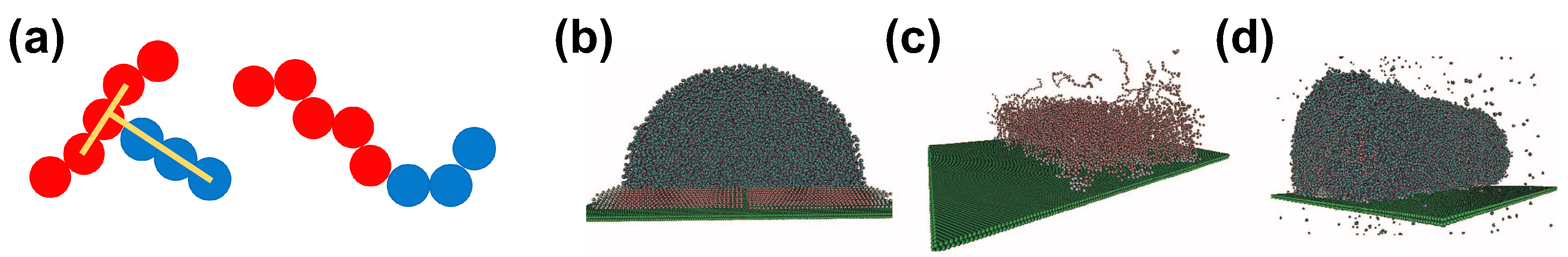
Figure 4.
The SAFT CG model. (a) SAFT CG model for water (one-bead–one-water and one-bead–two-waters models) and C10E4 surfactant. Transparent spheres indicate the CG beads and the atoms that they represent. Alkyl groups are in turquoise, ethoxy groups in grey and red beads represent the head groups. From Ref. [67]; (b) Experimental phase diagram for C10E4 surfactant and representative snapshots from simulation based on the SAFT CG model. From Ref. [67]; (c) Experimental phase diagram [110] for water–Silwet-L77 (superspreading surfactant) and representative snapshots from computer simulations based on the SAFT CG model. Colours indicate different parts (hydrophobic or hydrophilic) of the surfactant and water as indicated. Reproduced from Ref. [19] with permission from The Royal Society of Chemistry; (d) Surface tension versus surface excess concentration in the case of C10E4 surfactant. Open symbols correspond to experimental data [111], while filled circles are results obtained by simulation based on the SAFT CG model. From Ref. [67].
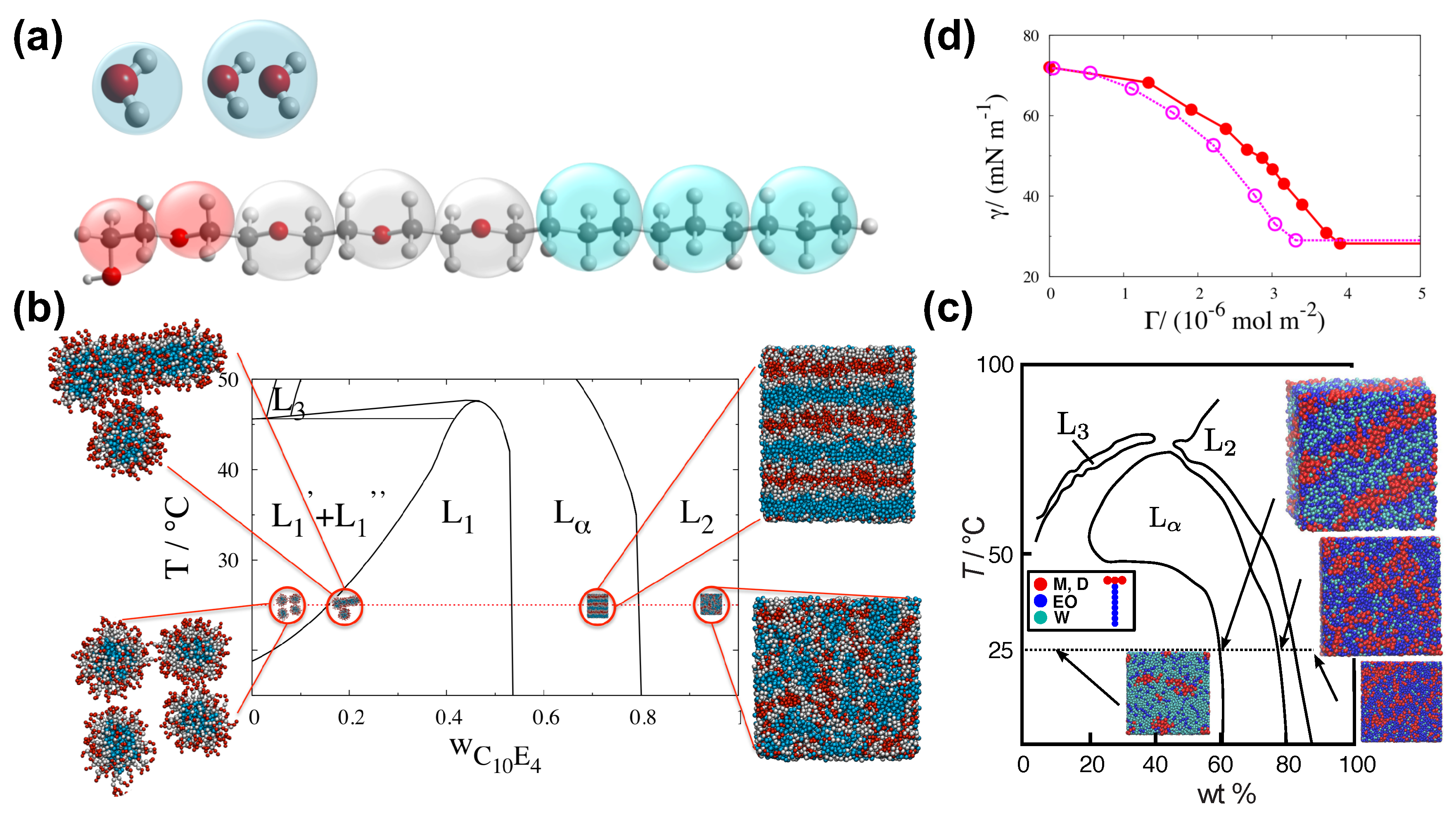
Figure 5.
Results from all-atom simulation. (a) Covered surface area by surfactant and related analysis based on advanced algorithms and Voronoi tessellation. Reprinted with permission from Ref. [21]. Copyright 2014 American Chemical Society; (b) Superspreading versus nonsuperspreading: Conformation of the droplet at the CL as suggested in Ref. [22]. (c) Surface tension obtained by experiment and simulation for different surfactants as indicated. Reprinted with permission from Ref. [21]. Copyright 2014 American Chemical Society; (d) Top view of the LV interface containing 18 surfactant molecules. From left to right: alkyl ethoxylate, trisiloxane, and perfluoroalkane surfactants. The hydrophilic part of the surfactants is in red, while the hydrophobic is in black. Water is omitted for the sake of clarity. Reprinted with permission from Ref. [21]. Copyright 2014 American Chemical Society.

Figure 6.
Results from all-atom simulation. (a) Final configuration of cylindrical water/trisiloxane and water/alkyl-polyethoxylate droplets on a SAM with a mole fraction of hydroxyl-terminated chains of . Reprinted with permission from Ref. [70]; (b) Contact angle versus time for different water/surfactant droplets on a graphitic substrate. The droplet size is about water molecules. Reprinted with permission from Ref. [70]; (c) Equilibrium configuration of water/trisiloxane droplets at 450 K on a hydroxyl-terminated SAM. Reprinted with permission from Ref. [70].

Figure 7.
Results from a bead–spring CG model. Different scenarios of spreading depending on the molecular architecture of the surfactant. T-shaped surfactant versus flexible linear surfactant. Reprinted with permission from Ref. [68]. Copyright 2005 American Chemical Society.
Figure 7.
Results from a bead–spring CG model. Different scenarios of spreading depending on the molecular architecture of the surfactant. T-shaped surfactant versus flexible linear surfactant. Reprinted with permission from Ref. [68]. Copyright 2005 American Chemical Society.

Figure 8.
Results from the SAFT CG model. (a) Time evolution of the spreading process for superspreading and nonsuperspreading surfactants at times , , and . Hydrophobic beads are in orange or red and hydrophilic beads are in blue. Cyan beads indicate the water molecules with each bead corresponding to two water molecules. Reprinted from Ref. [20]. Copyright 2015 American Chemical Society; (b) Schematic illustration of the leading adsorption processes during superspreading. The dominant direction of the adsorption is illustrated with a larger arrow end. The essential processes are the adsorption from the LV interface onto the substrate through the CL and the adsorption from the bulk to the LV interface. Reproduced from Ref. [19] with permission from The Royal Society of Chemistry. (c) The time evolution of droplet height during superspreading. Representative snapshots at each time are illustrated as indicated. Reproduced from Ref. [19] with permission from The Royal Society of Chemistry.
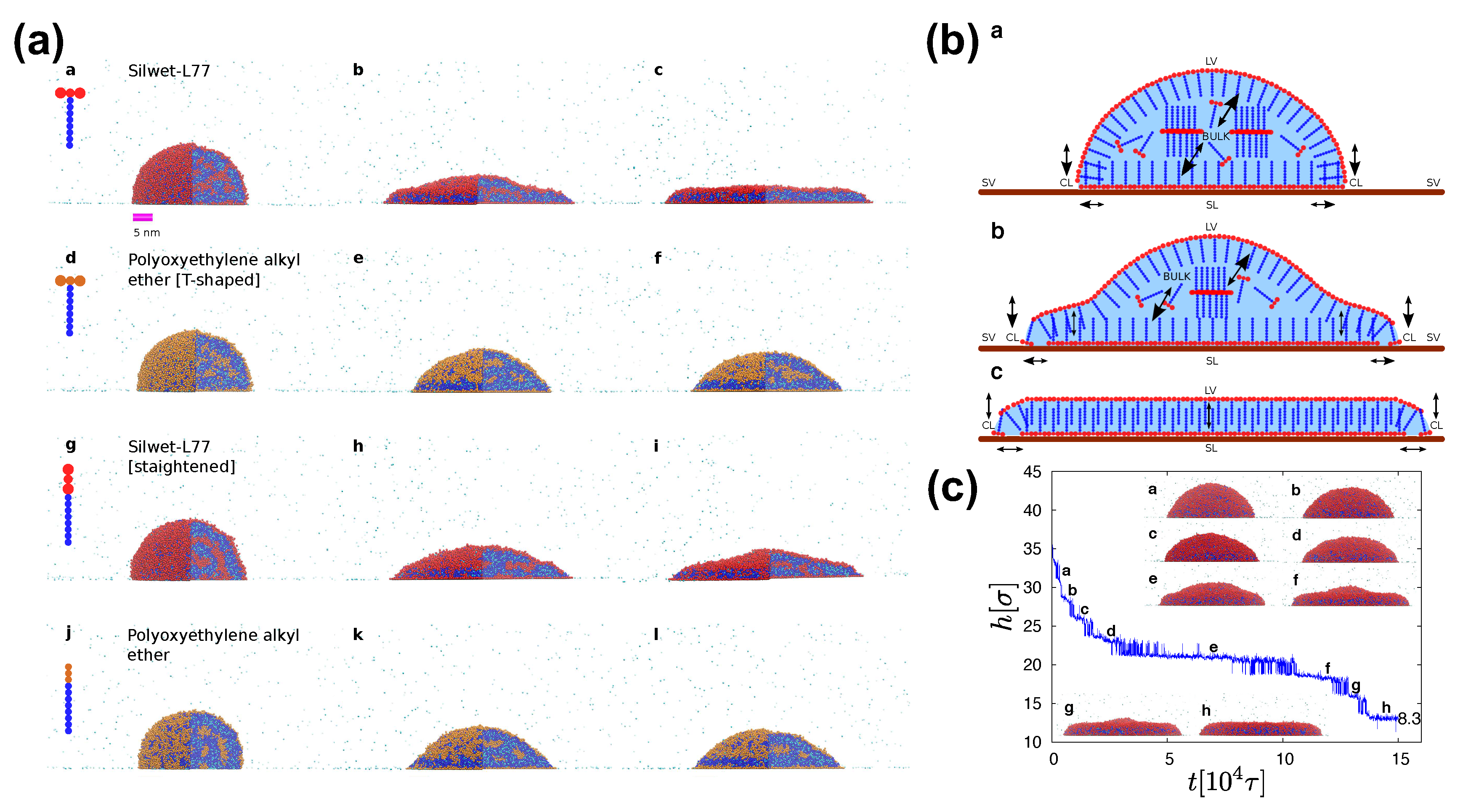

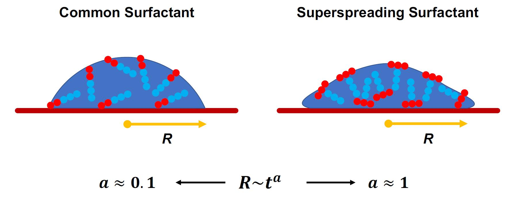
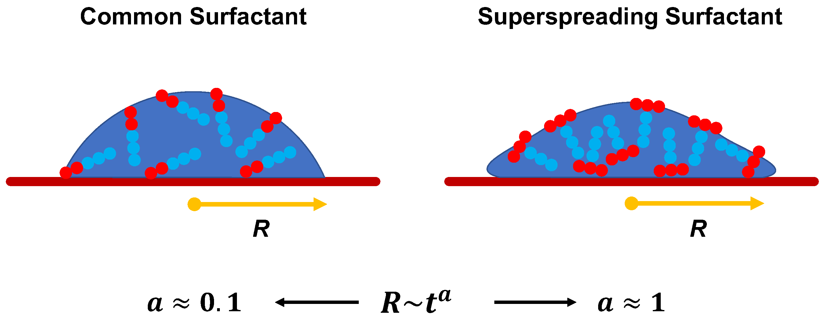
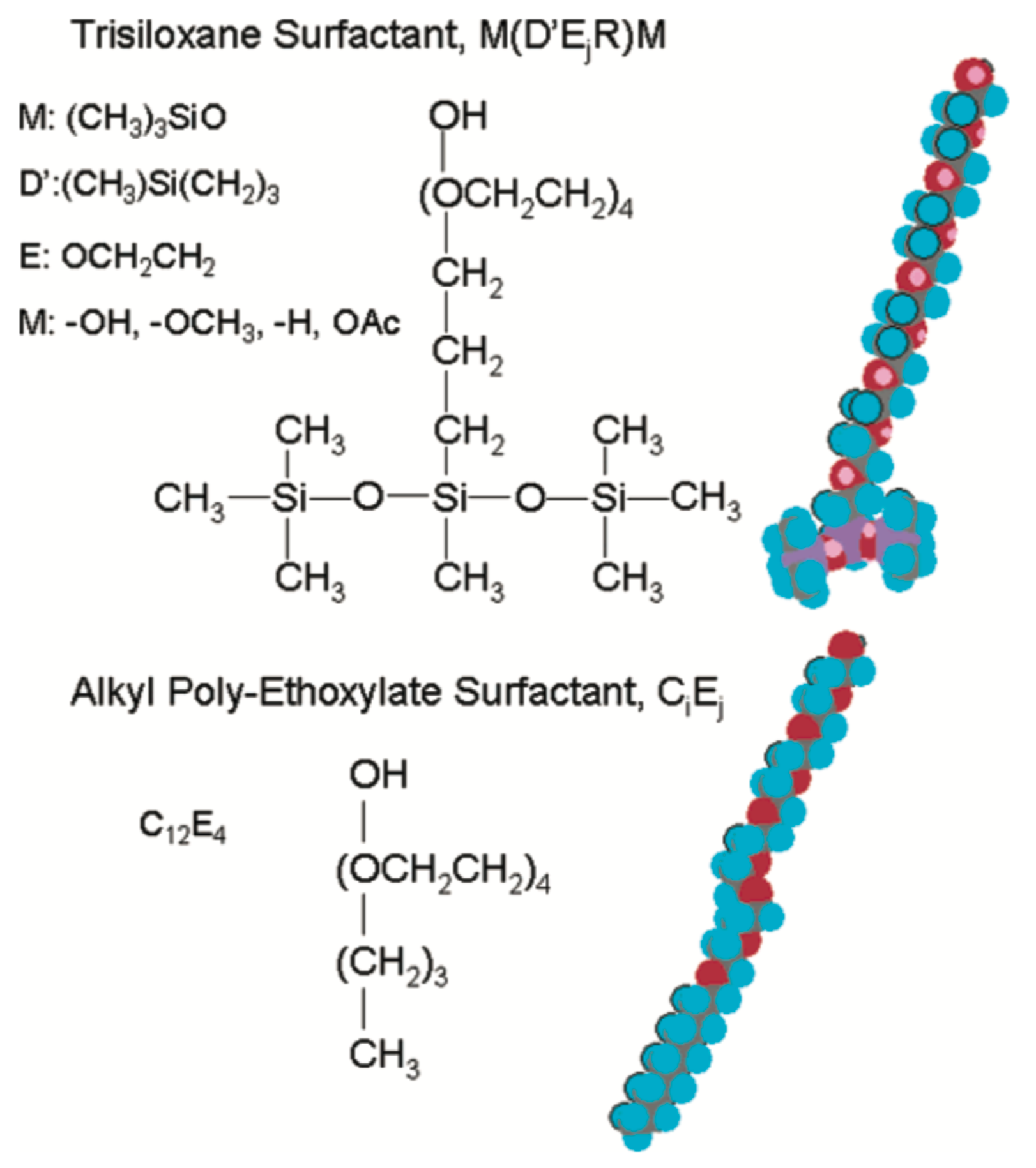
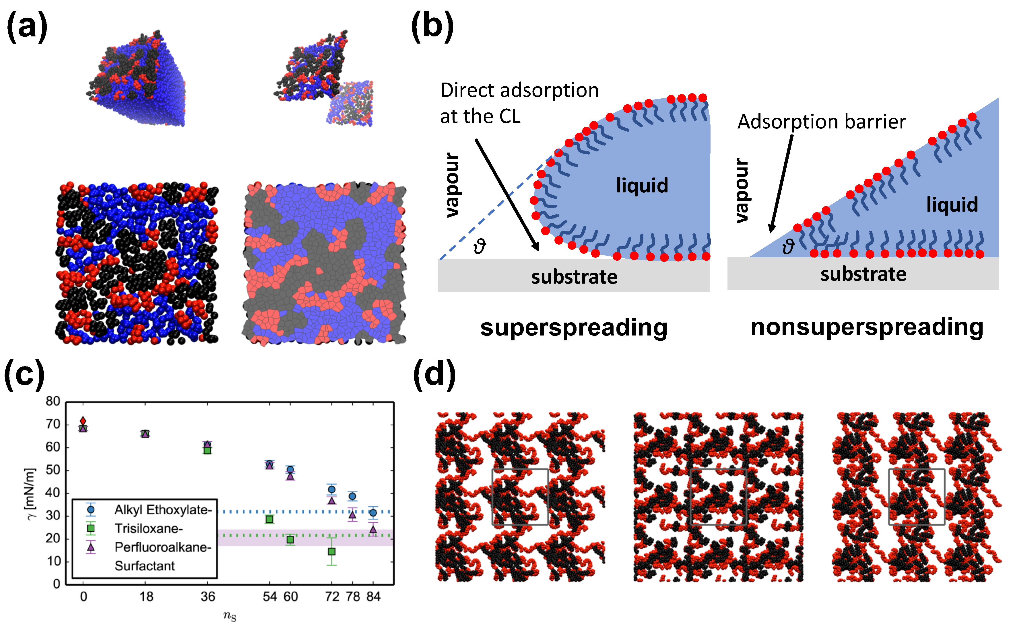
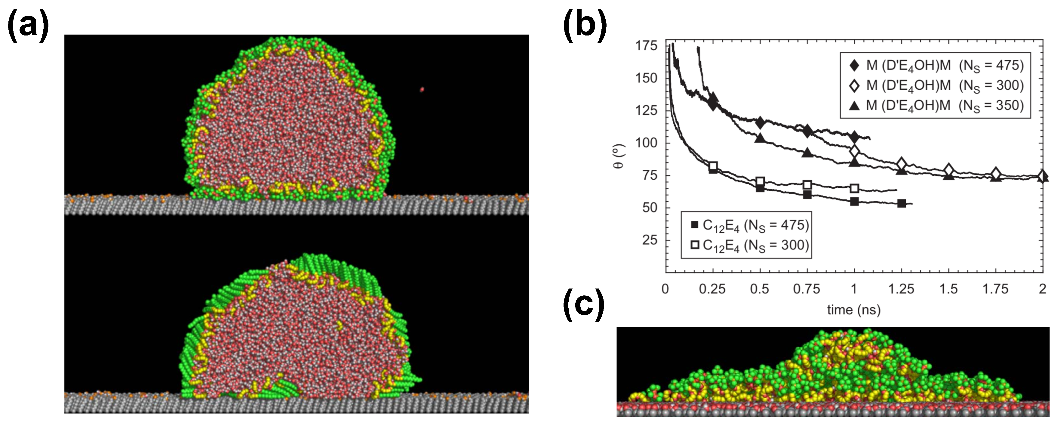
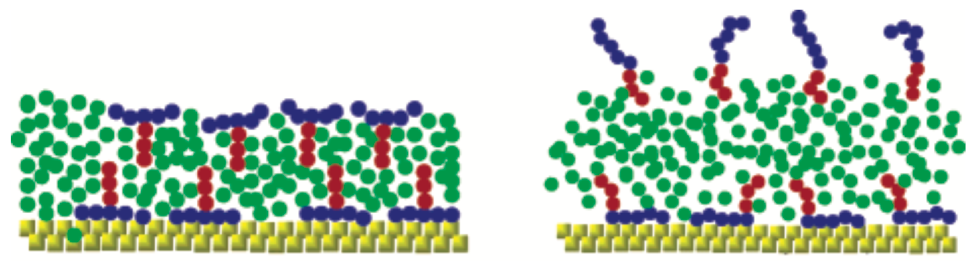
Table 1.
interaction coefficients between different components: type 1 for the hydrophilic head of the surfactant, type 2 for the hydrophobic tail, type 3 for the solvent, and type 4 for the substrate particles [68].
Table 1.
interaction coefficients between different components: type 1 for the hydrophilic head of the surfactant, type 2 for the hydrophobic tail, type 3 for the solvent, and type 4 for the substrate particles [68].
| Case 1 | ||||
| type 1 | type 2 | type 3 | type 4 | |
| type 1 | 0.1 | 0.1 | 3.0 | 2.0 |
| type 2 | 0.2 | 0.8 | 2.0 | |
| type 3 | 1.15 | 0.8 | ||
| type 4 | 1.0 | |||
| Case 2 | ||||
| type 1 | type 2 | type 3 | type 4 | |
| type 1 | 0.1 | 0.1 | 2.0 | 2.0 |
| type 2 | 0.2 | 0.8 | 2.0 | |
| type 3 | 1.15 | 0.8 | ||
| type 4 | 1.0 | |||
Table 2.
Mass in units m for different effective beads representing groups of atoms. See main text for details.
Table 2.
Mass in units m for different effective beads representing groups of atoms. See main text for details.
| Group of Atoms | Mass [m] |
|---|---|
| W | 0.8179 |
| M | 1.8588 |
| D | 1.6833 |
| EO | 1.0000 |
| CM | 0.9552 |
Table 3.
Mie interaction potential parameters in reduced units. for all cases. The length and the energy units are nm and K, respectively. Therefore, , which corresponds to 25 °C.
Table 3.
Mie interaction potential parameters in reduced units. for all cases. The length and the energy units are nm and K, respectively. Therefore, , which corresponds to 25 °C.
| i–j | |||
|---|---|---|---|
| W–W | 0.8584 | 0.8129 | 8.00 |
| W–M | 1.0491 | 0.8132 | 13.72 |
| W–D | 0.9643 | 0.6311 | 10.38 |
| W–EO | 0.8946 | 0.9756 | 11.94 |
| W–CM | 0.9292 | 0.5081 | 10.75 |
| M–M | 1.2398 | 0.8998 | 26.00 |
| M–D | 1.1550 | 0.7114 | 18.83 |
| M–EO | 1.0853 | 0.8262 | 22.18 |
| M–CM | 1.1199 | 0.7800 | 19.61 |
| D–D | 1.0702 | 0.5081 | 13.90 |
| D–EO | 1.0004 | 0.6355 | 16.21 |
| D–CM | 1.0351 | 0.5953 | 14.43 |
| EO–EO | 0.9307 | 0.8067 | 19.00 |
| EO–CM | 0.9653 | 0.7154 | 16.86 |
| CM–CM | 1.0000 | 0.7000 | 15.00 |
© 2019 by the authors. Licensee MDPI, Basel, Switzerland. This article is an open access article distributed under the terms and conditions of the Creative Commons Attribution (CC BY) license (http://creativecommons.org/licenses/by/4.0/).
Share and Cite
MDPI and ACS Style
Theodorakis, P.E.; Smith, E.R.; Craster, R.V.; Müller, E.A.; Matar, O.K. Molecular Dynamics Simulation of the Superspreading of Surfactant-Laden Droplets. A Review. Fluids 2019, 4, 176. https://doi.org/10.3390/fluids4040176
AMA Style
Theodorakis PE, Smith ER, Craster RV, Müller EA, Matar OK. Molecular Dynamics Simulation of the Superspreading of Surfactant-Laden Droplets. A Review. Fluids. 2019; 4(4):176. https://doi.org/10.3390/fluids4040176
Chicago/Turabian StyleTheodorakis, Panagiotis E., Edward R. Smith, Richard V. Craster, Erich A. Müller, and Omar K. Matar. 2019. "Molecular Dynamics Simulation of the Superspreading of Surfactant-Laden Droplets. A Review" Fluids 4, no. 4: 176. https://doi.org/10.3390/fluids4040176