Direct Numerical Simulation of a Warm Cloud Top Model Interface: Impact of the Transient Mixing on Different Droplet Population


1
Department of Applied Science and Technology (DISAT), Politecnico di Torino, Corso Duca degli Abruzzi 24, 10129 Torino, Italy
2
Department of Mechanical and Aerospace Engineering (DIMEAS), Politecnico di Torino, Corso Duca degli Abruzzi 24, 10129 Torino, Italy
*
Author to whom correspondence should be addressed.
Fluids 2019, 4(3), 144; https://doi.org/10.3390/fluids4030144
Submission received: 27 May 2019
/
Revised: 21 June 2019
/
Accepted: 25 June 2019
/
Published: 1 August 2019
(This article belongs to the Special Issue Multiscale Turbulent Transport)
Abstract
:Turbulent mixing through atmospheric cloud and clear air interface plays an important role in the life of a cloud. Entrainment and detrainment of clear air and cloudy volume result in mixing across the interface, which broadens the cloud droplet spectrum. In this study, we simulate the transient evolution of a turbulent cloud top interface with three initial mono-disperse cloud droplet population, using a pseudo-spectral Direct Numerical Simulation (DNS) along with Lagrangian droplet equations, including collision and coalescence. Transient evolution of in-cloud turbulent kinetic energy (TKE), density of water vapour and temperature is carried out as an initial value problem exhibiting transient decay. Mixing in between the clear air and cloudy volume produced turbulent fluctuations in the density of water vapour and temperature, resulting in supersaturation fluctuations. Small scale turbulence, local supersaturation conditions and gravitational forces have different weights on the droplet population depending on their sizes. Larger droplet populations, with initial 25 and 18 m radii, show significant growth by droplet-droplet collision and a higher rate of gravitational sedimentation. However, the smaller droplets, with an initial 6 m radius, did not show any collision but a large size distribution broadening due to differential condensation/evaporation induced by the mixing, without being influenced by gravity significantly.
1. Introduction
Atmospheric clouds play an important role in the evolution of the weather, both locally and globally, by influencing incoming and outgoing radiations, amount of precipitations and transport of water vapour, heat and other advected scalars like pollutant concentrations. Low altitude stratocumulus and cumulus clouds are formed on top of the planetary boundary layer. Various physical processes inside these clouds, which span over a wide range of temporal and spatial scales, need to be carefully modelled to improve weather predictions and climate modelling (see Pruppacher and Klett (2010) [1], Stull (1988) [2] and Devenish et al. (2012) [3]). Therefore, many studies have been devoted to analyzing each single aspects of the clouds.
The presence of a wide range of scales in an atmospheric cloud adds a layer of complexity to the micro-physical processes, which are linked to the droplet evolution. Droplet condensation/evaporation, dispersion, preferential concentration and transport processes are the key phenomena of the the micro-physical processes [3,4]. Many of these processes occur at the smallest scales of the flow [5], therefore, such processes need to be parameterized when the whole cloud or large scale modelling is considered [6,7]. Particle resolving direct numerical simulations (DNS), which aim to solve all the dynamically significant scales of a turbulent environment, have recently become a tool to investigate some of the cloud micro-physical processes using idealized atmospheric flow configurations.
In these simulations, it is not only necessary to solve all the turbulent scales down to the diffusive scales but it is also necessary to track the motion and the growth of every single cloud droplet in the fluid flow. Therefore, due to computational limitations, only a small portion of a cloud could be considered in a DNS study. The basic model used in all such works was introduced by Vaillancourt et al. (2001) [8]. In this model the Navier-Stokes (NS) equations with the Boussinesq approximation are solved for the air phase on an Eulerian grid, where the suspended cloud droplets are considered as inertial variable-mass points. The droplet model takes into account the variation of the droplet size due to condensation or evaporation according to the local supersaturation condition [1]. Most of such works focused on the simulation of a small portion of the well mixed cloud-core and introduced an external forcing to reproduce the inflow of energy due to the larger-scale cloud motions [9,10,11]. Other works have extended this methodology to investigate the effects of non-uniformity in the underlying turbulent flow and its consequences on cloud droplet micro-physical evolution. Such non-uniformity was introduced in the form of a turbulent kinetic energy (TKE) gradient and in the supersaturation distribution [12]. Götzfried et al. (2017) [12] and Kumar et al. (2014, 2017) [13,14] considered the evolution of a tiny cloud layer to analyze the cloud edge affects on the cloud droplet population, whereas Andrejczuk et al. (2004, 2006, 2009) [15,16,17] considered decaying moist turbulence with worm-like structures of supersaturated and subsaturated regions. Gao et al. (2018) [18] investigated the differences between cloud micro-physical evolution for various initial configuration of cloud and clear air layers, both in the presence and absence of forcing.
Entrainment and mixing in between supersaturated and subsaturated air parcels have long been considered important processes which shape the size distribution of the cloud droplets and therefore contribute to enhancing the collision rate [3]. Therefore, the understanding of cloud droplet evolution inside the mixing zone could contribute to bridge the gap between the condensational growth (effective for smaller droplets, below 10 m radius) and collisional growth (effective for larger droplets, above 40 m radius) [5,19]. In the mixing zone, two mechanisms contribute to the droplet micro-physics: (a) the presence of large fluctuations in the supersaturation, which broadens the size distribution of the cloud droplets by condensation/evaporation and (b) large accelerations in some localized regions of the flow [4,20], which can cause occasional collisions. Different scenarios can occur, which range between the two limiting mixing situations: (a) homogeneous mixing, where entrained air and cloudy air quickly mix at the small scale, so that the entire droplet population evaporate/condensate at the same time and (b) inhomogeneous mixing, where only a portion of the volume remains subsaturated/supersaturated and therefore, part of the droplet population quickly evaporate/condensate, whereas, the other parts of the population remains almost unaffected [21].
In this work, we studied the transient evolution of cloud water droplet populations inside a simplified top interface model of a warm cloud. The objective of this work was to investigate the differences in the micro-physical transient evolution of various cloud water droplet populations with sizes that approach the lower bound of the [15–40 m radius] [5] and sizes below the and their thermal feedback on the surrounding air. DNS using the Eulerian-Lagrangian model along with a collision detection algorithm (mostly neglected for this kind of study) was used for this work. Various thermodynamic processes, such as supersaturation, buoyancy, phase change of water vapour to liquid water and corresponding latent heat production, are interlinked by one-way coupling in between the cloud droplets and the surrounding fluid velocity and two-way coupling of the cloud droplets with the air temperature and the water vapour density. We investigated the transport inside a cloud interface characterized by a strong kinetic energy gradient (see also [12]). This configuration is known to generate a strong intermittent transient mixing layer [22,23,24] due to the entrainment/detrainment of fluid from/to the external regions [24,25]. This induces non-trivial complex behaviour in the droplet velocity distribution due to the interplay between larger scales and gravity, with little dependence on the Reynolds number [24]. Therefore, even if the Reynolds number which can be achieved in the direct numerical simulations is much smaller and not comparable with the real life cloud Reynolds number in the order of –, we think such simulations can still provide information that can be useful to understand some of the real cloud phenomena. The present simulations undergo a transient decay in TKE [12,15,25]. The methodology and the simulation set-up is presented in Section 2. Results presented in Section 3 include statistics and visualizations on the transient evolution of the fluid flow and the droplet populations and a discussion on the role of condensation/evaporation, sedimentation and collision on the evolution of the different droplet populations in the mixing layer separating the lower cloudy region from the upper clear air region.
2. Numerical Methodology and Simulation Setup
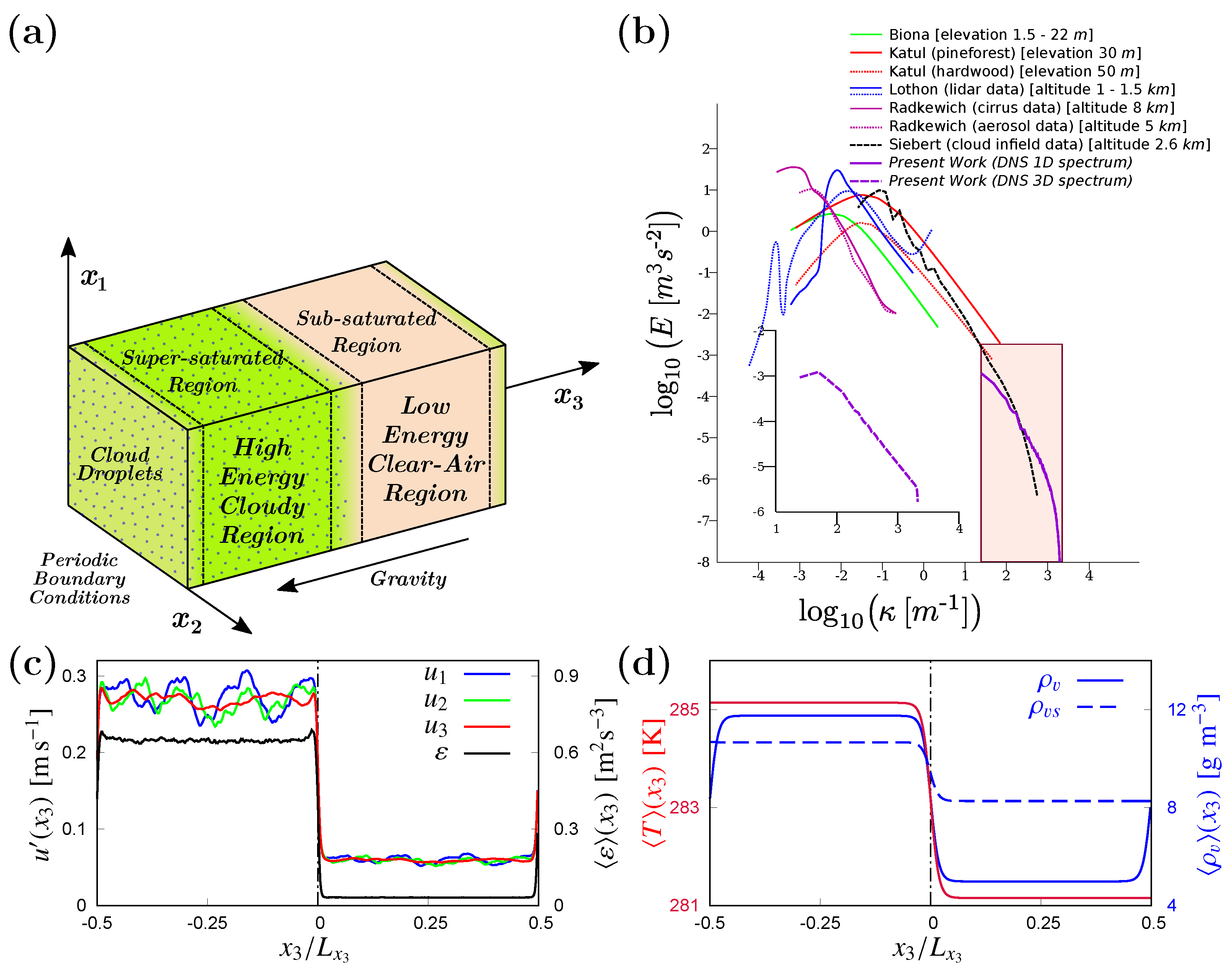
In this study, the interactions in between atmospheric low altitude warm cloud top and the above-lying clear air regions and its impact on cloud water droplets were simulated using DNS. Two cubic boxes, each with volume, representing warm cloud and clear air properties were combined together to create the simulation domain (see Figure 1a). The portion of the domain representing the cloudy air was seeded with a mono-disperse cloud droplet population. The airflow was modelled as an incompressible fluid flow according to the Boussinesq approximation. The governing equations for the airflow (carrier fluid) and the cloud droplets (dispersed medium) are presented below.
2.1. Evolutive Equations for the Fluid Flow
The numerical model for the evolution of the fluid flow considers NS equations for humid air, which are coupled with the Lagrangian tracking of every cloud water droplet, introduced in the initial condition. The numerical model of this study followed the model used by Vaillancourt et al. (2001) [8], later used by Kumar et al. (2014) [13], Gotoh et al. (2016) [26], Götzfried et al. (2017) [12] and Gao et al. (2018) [18]. The air phase equations use Boussinesq-like approximation and include the continuity and momentum balance equations for the airflow velocity and the temperature T and the water vapour density equations. Temperature and water vapour density were considered as advected active scalars. The fluid flow equations are
where is the temporal derivative, is reference mass density of air at temperature and pressure , is the pressure gradient, is the kinematic viscosity, is the gravity acceleration, is the thermal diffusivity of air, L is the latent heat for condensation of water vapour, is the specific heat at constant pressure and is the water vapour diffusivity. The “source” term in the momentum balance Equation (2) is B which represents the buoyancy force per unit volume due to small variations of temperature and water vapour density in the humid air. In the temperature (enthalpy) (3) and humidity (4) equations, the source term represents the condensation rate, that is, the local condensating or evaporating water mass per unit time and unit volume.
These source terms are expressed as
where is the reference temperature, is the reference water vapour density, is a constant dependent on the gas constants and of the water vapour and the air respectively, is the density of liquid water and is the radius of the i-th cloud droplet. The sum in is calculated on the droplets only within the (small) local volume V, where is the mass of the i-th droplet (in simulation, this volume is the volume of a computational grid cell). Droplet volume fraction (volume of droplets/volume of carrier fluid) for the largest initial droplet (initial radius, ) population is , which is considered as dilute suspension by Elghobashi (1991) [27], where the momentum feedback from the droplets (two-way momentum coupling) may be neglected. Therefore, in the computation of the buoyancy force, no momentum feedback from droplets to the fluid is considered, since in case of dilute suspension one-way coupling is prominent in between droplets and the surrounding fluid [27].
2.2. Lagrangian Equations for the Cloud Droplets
The Lagrangian descriptions of the cloud droplets consider them driven only by gravity and the Stokes drag law, since the droplet density is much higher than air density () and the Reynolds number of the droplet relative velocity with respect to the surrounding air is very small (after Pruppacher and Klett (1978) [1] pg 575 and Vaillancourt et al. (2001) [8], usually below 0.1). Moreover, their sizes change due to condensation/evaporation, driven by the local heat and water vapour diffusion around the droplets. Therefore, the equations for the i-th droplet are
where is the droplet position, is the droplet velocity, is the local relative humidity, is the saturation vapour density and is the droplet response time, which is
The droplet growth rate Equation (9) is dependent on the condition of surrounding relative humidity (Pruppacher and Klett (1978) [1], p. 511) and the proportionality coefficient C is defined as
where is the thermal conductivity of the air. As in Kumar et al. (2013) [10], we approximated in the definition of C.
2.3. Numerical Method of the DNS
Model equations for the fluid flow phase are solved using the Fourier–Galerkin (FG) pseudospectral method as in Iovieno et al. (2001) [28], while temporal advancement is approximated using a low storage second order Runge-Kutta (RK2) method with exponential integration of the diffusive terms [29]. The numerical code uses one dimensional (1D) slab parallelization using Massage Passing Interface (MPI) libraries. Dealiasing is carried out during data transposition. Discrete Fourier Transforms (DFT) are computed using FFTW subroutine library. Whereas, Lagrangian model equations for the droplets are solved in the physical space using the same RK2 method for temporal integration. After every time-step, droplets are exchanged among neighbouring processors according to their current respective positions. Fluid velocity, temperature and vapour density at particle positions are computed through a trilinear interpolation within each mesh cell, which is expected to be sufficient in the Lagrangian droplet model for . The feedback term is computed through cell average (particle-in-cell method). Higher order interpolation methods, for example, third order B-spline method would be optimal according to [30], in the sense that the interpolation error would be less than the discretization error. However, as outlined by Sundaram and Collins (1996) [31], the interpolation and the reverse interpolation schemes must be symmetric in order to guarantee energy conservation in the domain, so that the linear particle-in-cell reverse interpolation should be replaced with an equivalent higher order method (see for example [32]). The pseudo-spectral code used triply-periodic boundary conditions for all the fluid flow variables. A non-periodic temperature profile is introduced in the vertical direction by the decomposition ; where, the field , which contains the temperature fluctuations, is triply periodic but the full temperature field T is not periodic in the vertical direction. The sign of the temperature gradient determines the stability of the flow. Such decomposition of the temperature field modifies the temperature Equation (3) into
The code also includes a module for droplet-droplet binary collision detection, which assumes coalescence of the colliding droplet masses. After each time-step, the algorithm determines whether the distances between the pairs of droplet centers become smaller or equal to the sum of their redii by assuming a linear in–time variation of radius and position within the time-step. A collision between droplet i and j is considered to have occured if the first solution of lies between t and and their relative velocity is inward. Since the Weber numbers (ratio between the droplet kinetic energy and droplet surface energy) of the cloud water droplets are very small (), each collision is modeled as a successful coalescence in agreement with the experimental investigation of water droplet collisions by Rabe et al. (2010) [33]. Conservation of mass and momentum are then used to determine the size, position and velocity of the new droplet emerged from the collision.
2.4. Simulation Setup
The simulation domain replicates a small portion of a warm cloud top and layer of clear air above it. All interactions in between the cloud and the clear air happens through the interface formed by the edges of both the cloud and the clear air regions. Simulation parameters, constants and domain specifications used in our simulations are tabulated in Table 1. The values of the basic referred states correspond to the reference height of 763 m, which is a typical height for the low altitude warm clouds [34].
Table 2 summarizes the details of the simulation runs. In this simulation setup, an initial population of mono-disperse cloud droplets of three different size distribution are introduced in the cloudy volume of the simulation domain in three different simulation runs R25, R18 and R6; whereas, the carrier airflow initial conditions remained the same for all these simulations. A sketch of the simulation domain is shown in Figure 1a. Gravitational force (as presented in Figure 1a) acts on both the fluid flow (in form of buoyancy forces B in Equation (2)) and on the momentum of the cloud droplets in Equation (8). In this cloud top simulation setup, gravity therefore acts in downwards direction, causing heavier droplets to settle down towards the bottom boundary of the cloudy volume.
2.4.1. Initial Setup for the Fluid Flow
In field measurements of the cloud turbulent properties and associated clear air properties show different turbulent intensities, producing TKE gradients across the interfaces. Velocity fluctuations inside the cloudy regions mostly show higher TKE than that of the clear air region [34,35,36], which is mainly due to the instability of the moist air-mass, developed due to the buoyant updraft resulting in shear layer formation inside cloud [37]. This difference in kinetic energy is replicated by the average of velocity fluctuation root mean square (rms) distribution in the initial condition (Figure 1c) of present simulations. The clear air region of the simulation domain, shown in the right side region of Figure 1c is having lesser energy than the associated cloudy region (left side of the domain). The kinetic energy ratio between the cloudy domain and the clear air domain has been chosen to be around 20, which is in the range of the values which can be deduced from in-cloud measurements [34,35]. The thickness of the initial velocity fluctuations interface, measured as the distance between the horizontal planes where the difference of the TKE is 90% of the difference of kinetic energy between the cloudy and clear air regions, is about 0.006 m (see Figure 1c). Figure 1b presents few examples of spatial one-dimensional TKE spectra from infield measurements by Biona et al. (2001) [38], Katul et al. (1998) [39], Radkevich et al. (2008) [40], Lothon et al. (2009) [41] and Siebert et al. (2015) [42], to which the one dimensional initial TKE spectrum of present simulations has been superimposed (the three dimensional TKE spectrum is shown in the inset). Since in a DNS, we need to resolve Kolmogorov micro-scale , which also plays important role for the micro-physical evolution of cloud droplets [3,5], only part of the inertial sub-range and the dissipation range (up to the last three decades of TKE spectrum in logarithmic wave-number space) can be reproduced. The initial velocity field is generated by the superposition of Fourier modes with random phases, whose amplitude is determined from the following model 3D-spectrum
Coeffient controls the low wavenumber slope of the spectrum ( in present work). Coefficients A and control the variance and the initial correlation length and produces the exponential tail in the highest simulated wavenumbers approaching . The transition of initial fluctuations for airflow velocity from higher values inside the cloudy region to the lower values inside the clear air region of the domain was carried out using a linear superposition of the two initial cloudy and clear air isotropic field (see Tordella and Iovieno, (2006) [43], supplemental material of Tordella and Iovieno, (2011) [22] and Iovieno et al. (2014) [23]).
For this study, we selected an unstably stratified temperature profile, which can also be locally observed from small scale local temperature profiles obtained from in-cloud measurements (see Figure 2 of Ref. [34]). Initial temperature and water vapour fields are uniform on horizontal planes. No fluctuations of temperature and water vapour density were introduced in the initial conditions, so that the supersaturation fluctuations were generated only due to the mixing or due to the condensation/evaporation of the droplets to a minor extent. Therefore, any particle size broadening can be attributed to the non-uniform supersaturation field generated by the mixing process. Constants and in Equation (5) were chosen as the mean values of T and over the whole domain in the initial conditions. The thickness of the initial mean temperature and mean density of water vapour interface was slightly wider, around 0.007 m (Figure 1d). The initial mean density of water vapour and unstable mean temperature distribution inside the domain simulate supersaturated (relative humidity (RH) , 10% supersaturation) cloudy volume and subsaturated (, 40% subsaturation) clear air volume conditions. The supersaturated condition inside the cloudy region of the simulation domain will help the local cloud water droplets to grow by condensational deposition of water vapour on them; whereas, entrainment of the subsaturated clear air inside the cloudy volume can result in evaporative size reduction of the cloud droplets. These mean values of the supersaturation are around the upper estimation of the atmospheric measurements by Siebert and Shaw (2017) [44].
2.4.2. Initial Setup for the Cloud Droplets
A mono-disperse population of cloud water droplets of initial 25 m, 18 m and 6 m radii was initially introduced for the three simulations at random positions inside the cloudy part of the domain, that is, in the supersaturated region of the domain. The initial velocity of the droplets was set equal to the interpolated flow velocity at the droplet position.
Boundary conditions for the cloud droplets also follow periodic boundary conditions in the two horizontal directions, that is, droplets which exit the domain from horizontal boundaries re-enter from the opposite side with the same velocity as the fluid flow. However, the droplets settling on the bottom boundary of the simulation domain are removed from the simulation considering that those droplets are no longer present inside the cloudy volume. In this way, they do not re-enter the simulation domain from the top in the clear air region above the cloud. This choice has some positive as well some negative impact on the statistics of the simulated cloud droplets. Due to gradual removal of the heavier droplets from the cloudy portion of the domain, the number of samples for averaged droplet quantities were reduced near the bottom zone of the cloudy volume. However, simultaneously the cloud droplets were prevented from reappearing inside the clear air part of the domain caused by the periodic boundary conditions. This setup prevented any spurious droplet feedback to be present on the fluid volume near the top of the clear air region. Evaporation of the liquid water from the droplets results in size reduction. In the case of a droplet reducing below 4% of their initial radius, it was assumed that the droplet was completely evaporated within one time-step. This avoids the numerical instability of the small droplets, which have time-scales much smaller than the Kolmogorov time-scale.
3. Results of Transient Evolution
3.1. Time Evolution of the Fluid Flow
Since no external forcing has been introduced, the only force that can amplify the velocity of the fluid flow is the buoyancy force generated by the variations of temperature and water vapour density in the humid air. Transient evolution of the volume averaged quantities, such as TKE E, its dissipation rate , Taylor micro-scale Reynold’s number and integral length scales L exhibit transient decay or growth with time as shown in Figure 2. Turbulent fluid statistics along anisotropic direction is carried out by plane averaging across homogeneous horizontal planes. For computation of volume averaged turbulent quantities , the plane averaged quantities are averaged over the bulk of the cloudy region [] and the clear air region []. The definitions for E, , , and L are given as
where is the average of rms velocity fluctuations along two homogeneous directions () along which flow should remain homogeneous and isotropic, since the only sources of in-homogeneity and anisotropy are gravity and energy/temperature/density of water vapour gradient, which are acting along vertical direction; and is the velocity correlation function [45]. Evolution of E and is plotted in Figure 2a using logarithmic scale in the both axes. More than the half of the initial E and inside the cloudy region is lost during the first 0.3 s, after which the evolution of the E and follows a power-law scaling with time (with scaling exponent of −1.25 for E and −2.25 for ).
Figure 2b presents time evolution of , which shows two phases in its evolution inside the cloudy region. During the first phase till 0.3 s of initial transient, turbulence develops from the initial random conditions. Initially a increase in is observed due to the rapid increase in spatial scales (such as ) compared to the decrease in E with time. This is followed by a sharp decrease in , due to the rapid decrease in E with time which dominates over the the increase in . During the second phase, E decays at and grows as , which results in a gentle decay of at . Since decrease in E inside the clear air region is much slower than the increase in its spatial scales and the detrainment of E happens from the cloudy to clear air region; the evolution of in clear air shows increment for longer duration compared to the cloudy region, which is followed by a slow decrease.
For calculation of the integral length scales L, both longitudinal and transversal integral scales are computed along the two homogeneous directions and averaged. In Figure 2c, the transversal length scales are not exactly one half of the longitudinal length scales, which is an indication of anisotropic evolution of the flow across the domain with time. The effect of the numerical boundary of the domain also influenced this anisotropic evolution of the integral scale, since the scales can not grow beyond the domain size. The decay in kinetic energy also produces a growth of the Kolmogorov micro-scale . The resolution of the simulation increases with time, since varies from 1.0 at the beginning to 3.7 at the end of the simulation inside the cloudy region of the domain (inside clear air region, always). The growth of the also produces a transient evolution in the average droplet Stokes number and the settling parameter of the different droplet populations in the domain, as shown in Figure 2d. is a ratio between the droplet response time in Equation (10) and the Kolmogorov time scale and is a ratio between and , where is the terminal velocity of a droplet and is the Kolmogorov velocity. Due to decay in the kinetic energy (and the corresponding growth in ) in the domain, the droplets become gradually less and less sensitive to the turbulence (indicated by the transient growth of the parameter), whereas, the droplet Stokes number gradually reduces.
Figure 3 presents the time evolution of air statistics. Time has been re-scaled using the initial eddy turnover time taken at 0.043 s, which is 0.115 s, in order to reduce the influences of the initial evolution of the flow. Since all the three different simulations were initialized with same initial background fluid flow conditions, similar transient evolutions are observed for various fluid turbulent quantities. In transient evolution of in Figure 3a, detrainment of TKE to clear air region of the domain is observed to happen through the interface (dotted line in the middle) and also through the top boundary on top of the clear air region of the domain (due to periodic boundary condition, which generates a secondary inhomogeneous layer). Detrainment of TKE and widening of the TKE interface towards the clear air region of the domain can be recognized by following the positions of the kurtosis peaks of vertical component of fluid velocity in the Figure 3b, which moves toward the core of the clear air region. Skewness and kurtosis of the fluid quantities are computed using horizontal plane averages as a function of vertical direction . After 6 initial eddy turnover time (), overall TKE and the amplitude of the kurtosis peaks are observed to become lower. During the final stage of the simulation (), negligible TKE is left inside the fluid motion and the smaller peaks of kurtosis represent a well mixed stage in distribution of rms of velocity fluctuations throughout the domain. Decay in kinetic energy is reduced by the production of buoyancy inside the mixing layer. Unstably stratified temperature profile in the vertical direction amplifies vertical motion (see also Gallana et al. (2014) [46]) and the fluctuations of and T produce buoyancy fluctuations (Equation (5)), which introduce energy into the vertical motion (Equation (2)). This cumulative effect becomes visible after (see the growth of in the mixing region in Figure 3a), when the flow lost most of its initial kinetic energy. This source of kinetic energy accelerates the growth of the mixing layer and reduces the extent of the undiluted regions as well. During the later stage of evolution, , the initial configuration of two different regions is no more distinct and the flow begins to approach a homogenized state.
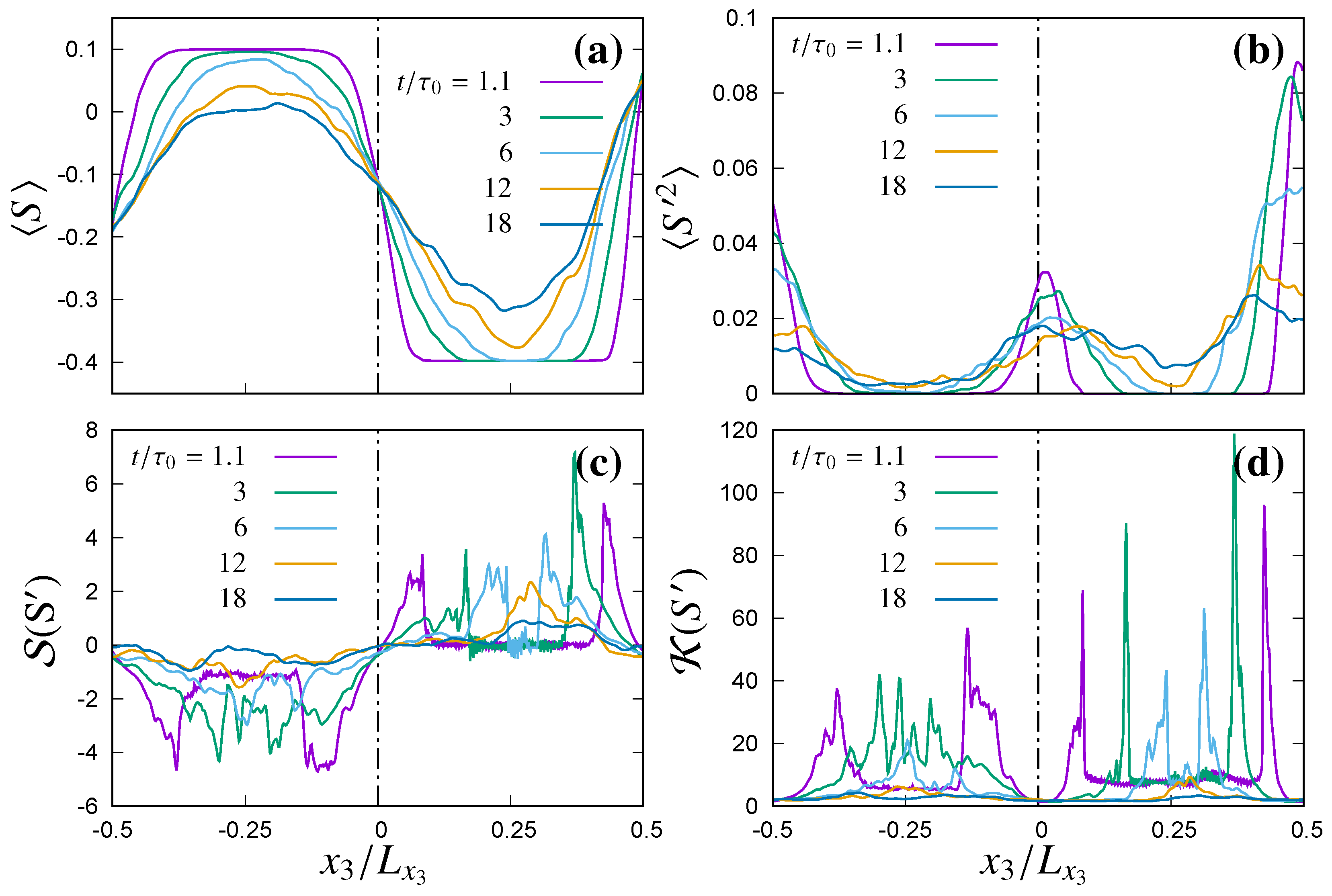
Figure 3c,d presents the time evolution of the mean of water vapour density and temperature profiles respectively. Mean of both the density of water vapour and temperature decrease inside the cloudy region of the domain, whereas, it increase inside the clear air region. The resulting profile of mean supersaturation (which is initialized with a magnitude of 10% inside the cloudy region and −40% inside the clear air region) shows a decrease in its magnitude inside the supersaturated cloudy region and an increase inside subsaturated clear air region (Figure 4a). The mixing process tends to produce a uniform supersaturation profile, therefore, during the final stage (), the mean supersaturation value remains positive () only in the central part of the cloudy region, whereas, most of the domain is subsaturated (). Figure 3e,f present the time evolution of the variance of water vapour fluctuations and temperature fluctuations . Resulting variance in plane averaged supersaturation fluctuations is shown in Figure 4b. Though no fluctuations are introduced in the initial condition for the temperature and the density of water vapour, fluctuations are generated by the mixing in the interface region and are propagated inside the undiluted core of the cloudy or the clear air region gradually with the spreading of the mixing region. A minor source for the fluctuations in the fluid flow quantities is the droplet feedback term in Equations (3) and (4). However, since the mean condensational time-scale is much larger than the eddy turnover time-scale, gives an overall small contribution for generating fluctuations. In Figure 3e and Figure 4b, two peaks (one in the interface in the middle of the domain and another one near the bottom and the top boundaries) are observed in the fluctuations of the density of water vapour and supersaturation, due to periodicity in the initial density of water vapour condition. However, since the initial temperature is non-periodic in the vertical direction and varies only at the mixing interface in the middle of the domain, Figure 3f shows only one peak in the variance of the temperature fluctuations. Temporal growth of the scalar (density of water vapour, temperature and supersaturation) mixing layers and widening of the scalar interfaces are evident from the shift in the peaks of the skewness and kurtosis of the scalars towards the undiluted central regions as shown in Figure 3g,h and Figure 4c,d, which gradually decrease in magnitude with mixing spreading all across the domain.
Figure 5a,b presents the time evolution of one dimensional (1D) horizontal spectrum of the vertical component of air velocity in the wavenumber space k, sampled at the middle horizontal plane of the initial configuration of the cloudy region and at the middle plane of the initial interface region (with 3 adjacent plane averaging in both cases). The 1D spectra in wavenumber space distributed in the homogeneous directions is computed as
where is the number of grid points in direction, is the Fourier transform of quantity f. Since initially the cloudy and the clear air region were initialized with two homogeneous and isotropic turbulent cubic domains with a TKE ratio of 20 in between the two regions, the initial 1D transversal spectra for all the three components of velocity fluctuations looks almost similar (some differences can be observed in the lowest wavenumbers due to smaller number of samples). The interface region in the initial condition contains lower TKE than that of the cloudy region of the domain (due to linear interpolation in TKE magnitudes in between the cloudy and the clear air region), which can also be observed in the initial TKE spectra of the interface showing vertical shift downwards than that of the cloud core region. With time advancement, the dissipative wavenumber range from the initial condition shows transition towards smaller wavenumbers indicating growth in the Kolmogorov micro-scale with time, gradually shrinking the inertial sub-range. Moreover, the spectra of different components of velocity fluctuations do not replicate each other during the later instances of the simulation, resembling an anisotropic time evolution of the fluid flow.
In Figure 5c,d, the transient evolution of the water vapour density fluctuations spectra and in Figure 5e,f, temperature fluctuations spectra in wavenumber space k is presented, sampled at the cloud core and the interface. Presence of a mean gradient in the initial scalar profiles along the vertical direction creates a large variance of that scalar in the mixing layer (Figure 3), which is observed to spread towards the undiluted regions with time. Since the mean gradient in the mixing region is large enough to produce sufficient variance in the scalars to counter its dissipation and the turbulent transport, a well mixed region is observed to be created with a scalar spectrum quickly approaching Kolmogorov inertial range [23]. Initially the only source of temperature and density of water vapour variance inside the undiluted cloudy region is the droplet condensation/evaporation. Therefore, initially the scalar spectra are not well developed but after , the growth of the mixing layer gradually destroys the cloudy region, so that similar scalar spectra like the mixing region are replicated inside the cloud core as well.
3.2. Time Evolution of the Cloud Droplet Population
The three simulations of this study are initialized with three different mono-disperse cloud droplet populations as enlisted in Table 2. The droplet populations go trough distinct transient evolution according to their surrounding fluid flow conditions. In general, droplets in the cloud core experience an average condensational growth due to supersaturated ambient, whereas, the droplets exiting the cloud core region, tend to evaporate due to subsaturation. A visualization of the flow is shown in Figure 6, where enstrophy () of the fluid field across a vertical plane (plane ) is presented with superposition of the cloud droplets around that plane (thickness of droplets containing slice is 0.0025 m) after 6 initial eddy () turnover time and along with the supersaturation S field in contour lines. The line at marks the extent of the cloudy region, where condensational growth occurs. In the region with , droplets would instead experience a quick evaporation. Although almost similar, small differences in the local enstrophy can be observed as a consequences of the cloud droplet feedback term in Equations (3) and (4), which determines also the buoyancy term B in the momentum balance Equation (2). Since buoyancy is sensitive to the small local fluctuations in the density of the water vapour and temperature T, differences in droplet feedback due to different droplet sizes (Equation (6)) can result into differences in the local fluid velocity, although the initial fluid flow conditions are identical. Distribution of enstrophy in Figure 6 gradually decreases with time, as TKE distribution also decreased as shown in Figure 2a and Figure 3a. Due to differences in the cloud droplet Stokes number as shown in Figure 2d, droplets show different responses to the local enstrophy field. In Figure 6a, droplets of initial 25 m mono-disperse distribution can be seen to preferentially concentrate away from the regions of higher enstrophy and often forming string like patterns and clustering in the areas of lower enstrophy. However, the gradual reduction of the average Stokes number with time reduces the tendency to cluster, while gravitational settling, droplet size broadening reduce correlation between the droplet concentration and the local strain. A similar but much milder tendency can also be observed in Figure 6b for the simulation with an initial 18 m mono-disperse droplet population. On the contrary, a higher uniform concentration can be seen in Figure 6c for the droplet population with initial 6 m radius.
At the same time, droplets undergo gravitational sedimentation which is only partially counterbalanced by turbulence. The relative importance of sedimentation is controlled by the dimensionless settling parameter [19]. Since decays as in these present simulations, the importance of gravitational sedimentation grows with time (see Figure 2d). Larger droplets (initial 25 m radius population) begin to gather at the bottom of the domain from the beginning of the simulation and rarely enters the mixing layer (Figure 6a). Droplets with initial 18 m radii have a comparatively slower rate of sedimentation and are observed to cross the cloudy region border through detrainment process (Figure 6b). On the contrary, smaller droplets (initial 6 m radius population) do not show significant sedimentation. They are observed to easily diffuse in the clear air zone (Figure 6c), where, due to their shorter evaporation time-scale (proportional to ) and longer residence time (roughly proportional to but modified by the droplet settling velocity ), they can completely evaporate. Moreover, for the smaller droplet population, the presence of strong subsaturation near the bottom boundary and at the clear air region of the domain also removed droplets by complete evaporation. This evaporation contributes to cool down the subsaturated layer above the mixing region, increasing the negative buoyancy [7] and thus enhancing the mixing process. Whereas, for the larger droplets, after a few initial time-scales, this process of detrainment to subsaturated clear air zone and complete evaporation of the droplets is not present.
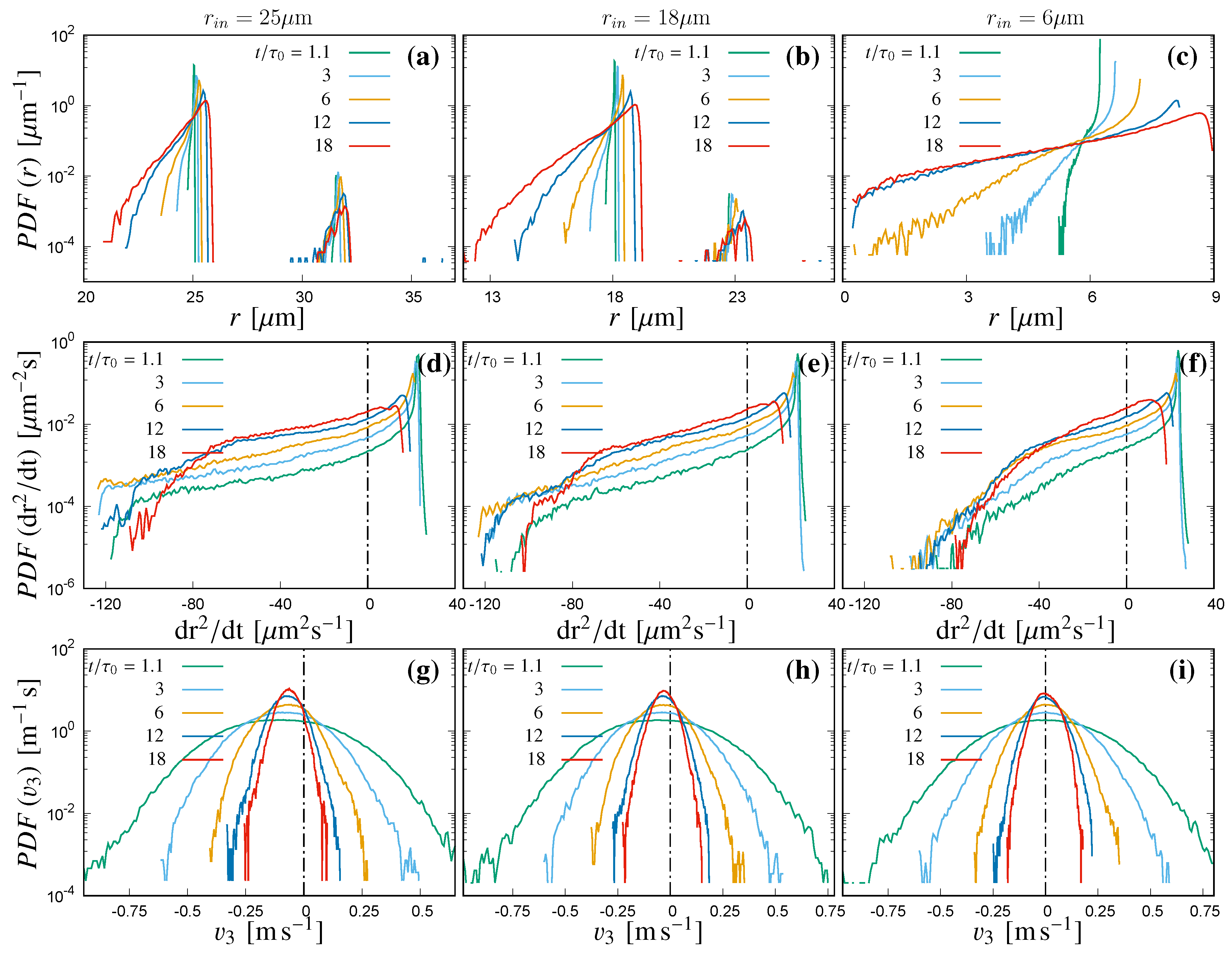
This is reflected in the transient evolution of normalized probability density functions (PDFs) of the droplet size, velocity and growth rate; which are presented in Figure 7. Figure 7a–c present the evolution of PDFs of the cloud droplet radius with time. Both the cloud droplet populations with initial 25 and 18 m radius show limited broadening of their sizes due to condensation/evaporation and the presence of two secondary peaks which correspond to the collisions (Figure 7a,b). However for the droplet population with initial 6 m radius, no collisional growth is observed to happen during the simulation duration. Whereas, the width of the DSD due to both the evaporation and condensation processes is observed to be wider in Figure 7c and certain number of droplets are observed to evaporate completely. The impact of condensational size growth or evaporative size reduction is more efficient for the smaller droplets (since droplet radius growth rate is proportional to , see Equation (9)). PDFs of , which indicates the growth rate in the droplet surface area, are presented in Figure 7d–f. As from Equation (9) is proportional to the local supersaturation , simulations of the three initial mono-disperse cloud population should exhibit similar transient evolution, since the background supersaturation spatial distribution is similar for the three simulations. However, droplets experience different supersaturation conditions due to their different paths, which also depends on their individual sizes and the local air conditions. Smaller droplets of initial 6 m radius do not show the extreme negative tail of as observed for larger droplets in Figure 7d,e, because this leads to a complete evaporation of the droplets (Figure 7f).
Moreover, since subsaturation can result in highly negative for the sub-micron droplets from the initial 6 m droplet population and since the numerical time-step for the sub-micron droplets needs to be very small and their micro-physics cannot be modelled using Equation (9); the droplets with sizes below 4% (≤0.24 m) are removed.
Due to gravity, vertical component of the cloud droplet velocity can exhibit different behaviour compared to the velocity components along the horizontal directions. Transient evolution of PDFs for is plotted in Figure 7g–i. During the early stage of evolution, the PDFs of shows wider distribution due to the presence of TKE inside the domain, influencing the droplet velocity as well. However the decay of TKE narrows the spectrum of and therefore with time. The gravitational settling is visible in the shift of the maxima of the PDFs of toward the negative values for the larger droplets. From Figure 7g, most of the cloud droplets of initial 25 m population are observed to have higher negative during the later instances of the simulation. Free fall velocity for a 25 m cloud water droplet is 0.077 m/s and the peak of the PDF of of this population is observed at 0.063 m/s after the first time-scale, which is implying dominance of gravitational settlement with velocities close to the free fall condition. Simulation with initial 18 m population (Figure 6b and Figure 7h) is observed to comparatively settle down slowly than the initial 25 m population. However, the simulation with initial 6 m population shows almost symmetric evolution of around the zero (Figure 7i), which indicates negligible effect of gravitational acceleration on this cloud droplet population.
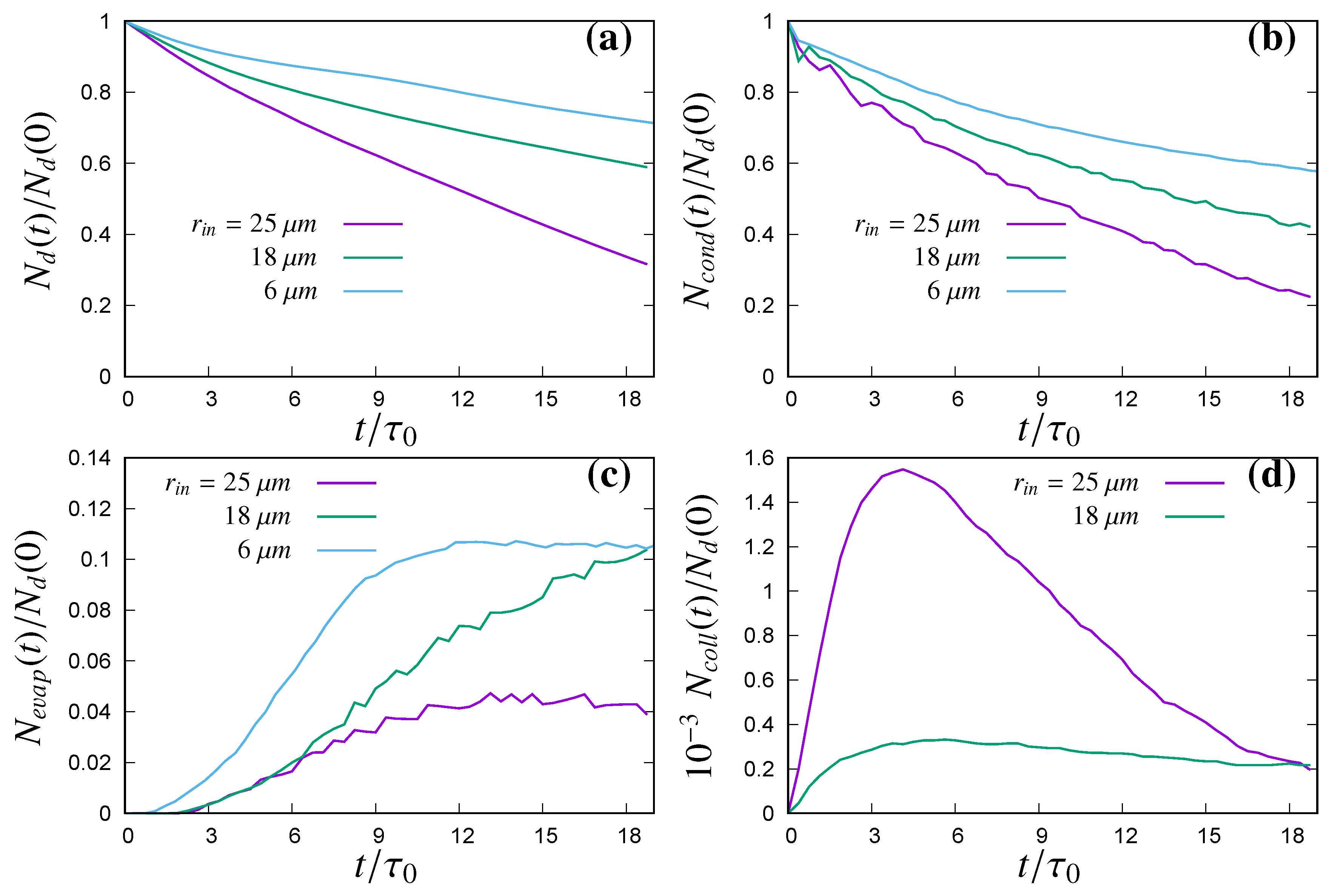
The number density of the droplets inside the simulation domain can change with time due to collisions or complete evaporation of the liquid water or due to gravitational sedimentation of the droplet out of the domain bottom boundary. To quantify the relative importance of condensation, evaporation, collision and gravitational sedimentation; the transient evolution in the number density of droplets is presented in Figure 8. Evolution in number density of all droplets (normalized by initial droplet number density ) is presented in Figure 8a, where most significant reduction in total number of droplets can be observed for the initial 25 m droplet population and comparatively less for the initial 18 m droplet population and much lesser for the initial 6 m droplet population. The most active physical process to result in reduction of the total number of cloud droplets for the initial 25 and 18 m droplet populations is the gravitational settling and subsequent removal of the droplets falling below the bottom boundary of the domain. However, the most active physical process for the initial 6 m droplet population, reducing the total number of droplets is the complete evaporation. In Figure 8b, time evolution in the normalized number density of the droplet population remaining to its initial radius or exhibiting size growth due to condensational water vapour deposition is presented (, where corrospond to radius of a droplet after first collision with a similar sized droplet). Though, the initial 6 m droplet population did not exhibit any collisional growth but some fraction of the population grew more than size due to higher degree of condensational growth. Transient evolution in the normalized number density of the cloud droplets experiencing evaporative size reduction is presented in Figure 8c. For the initial 25 m droplet population, droplets with a radius smaller or equal to 24.5 m are considered for counting the number density of evaporating droplets (17.5 m for initial 18 m population and 5.5 m for initial 6 m population). The effect of complete evaporation for the initial 6 m droplet population is evident from Figure 8b where the number density of the droplets that is equal to, or larger than, the initial 6 m size is observed to decrease with time but in Figure 8c the number density of evaporating droplets during the later stage of the simulation is almost steady, implying some physical process is resulting in the removal of droplets in the evaporating range. In Figure 7c, the absence of sub-micron droplets is seen to happen from 12 to 18 initial eddy turnover time, which also confirms the presence of the complete evaporation of sub-micron droplets for initial 6 m droplet population. The initial 25 and 18 m droplet population shows growth in the DSD due to occurrence of collision in different size ranges. Figure 8d presents normalized number density of the droplets in size ranges corresponding to collision between two similar sized droplets (secondary peaks in Figure 7a,b). For this transient evolution of the number density of colliding droplets, the source is the occurrence of collisions but the sink is the gravitational sedimentation of the droplets out of the domain. For both the initial 25 and 18 m droplet population in Figure 8d, during the initial 4 initial eddy turnover time, occurrence of collision dominates over the gravitational sedimentation but later the droplets with 1 collision for 25 m initial droplet population are removed from the domain very rapidly, whereas for the 18 m initial droplet population, the number of droplets with 1 collision remains almost steady. The occurrence of collision in between larger sized droplets (already with one collision) to the smaller droplets resulting in droplets with two or more collisions was very rare and happened mostly in the case of 25 m initial droplet population.
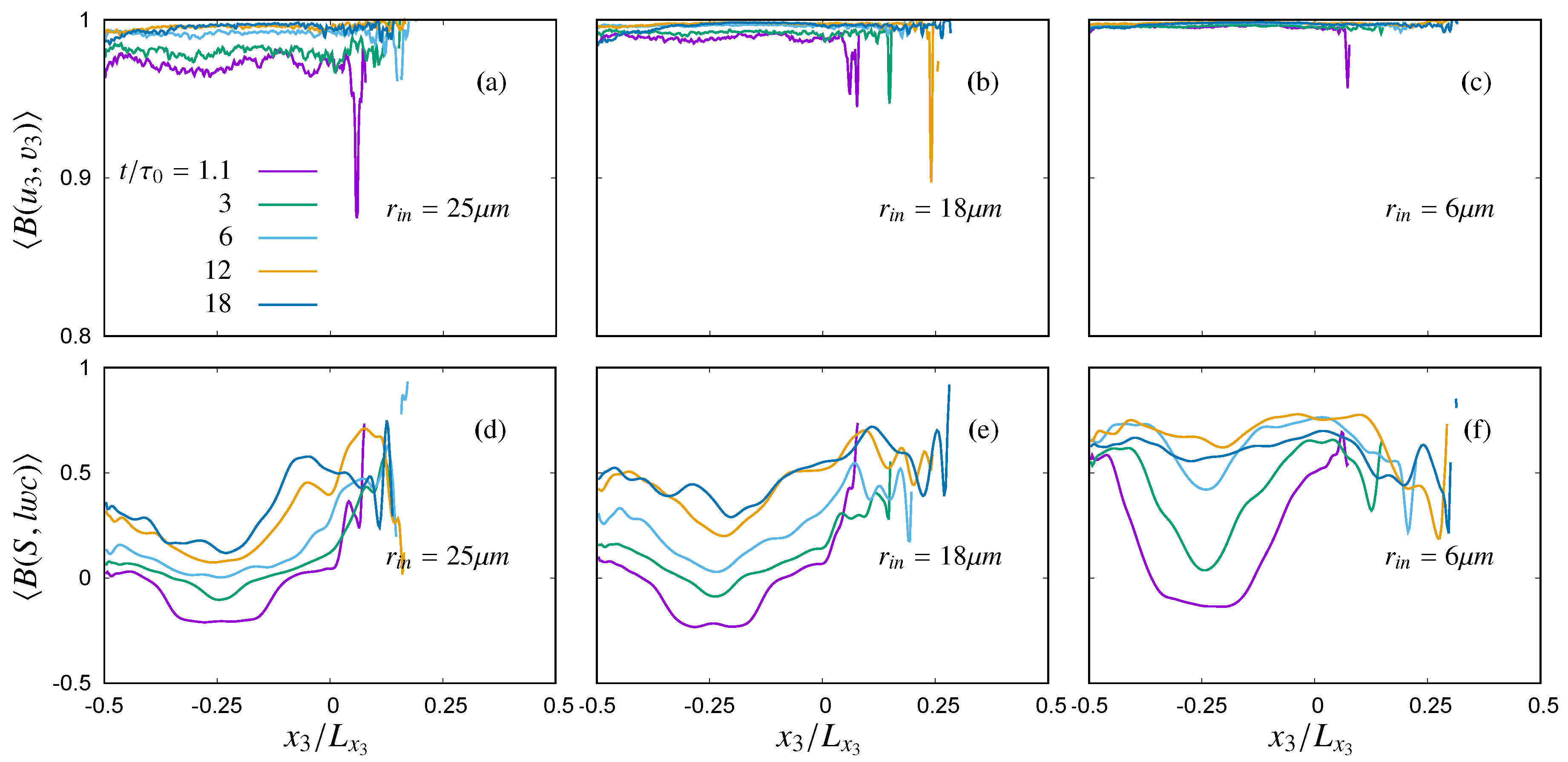
Time evolution of the one-point correlation between fluid flow and cloud droplet (where a and b are fluid and droplet quantities respectively) is presented in Figure 9. Since the droplet distribution is not uniform, for the calculation of these correlation parameters, both the fluctuations in the cloud droplets and fluid flow quantities are plane averaged in horizontal directions , considering only grid cells containing cloud droplets withing its volume and the droplet quantities are averaged to the corresponding grid points. In the correlation between the fluctuations in the vertical component of fluid velocity and droplet velocity in Figure 9a–c, and are very well correlated for initial 6 m droplet population but less correlated for 18 m and lesser for 25 m initial droplet population during the initial instances. Spurious fluctuations in correlation parameters are observed in the interface region, where number of droplet samples are much smaller. Since TKE inside the domain during later instances was much smaller and the Stokes numbers decreases (Figure 2d), as well for all the populations, the velocity fluctuations for both the fluid and the droplet tend to correlate more with time advancement. In Figure 9d–f, correlation between the supersaturation fluctuations and fluctuations in liquid water content is presented. Due to particle clustering and high fluctuations in the size of the statistical samples, bezier smoothing has been applied to the correlation in between and . This smoothing significantly modifies the data only in the clear air region of the domain, where number of droplets are very small. Improved statistics could be obtained by considering ensamble averaging between different simulations with independent initial conditions. Since initially inside the undiluted cloudy part of the domain, was 0 and gradually the fluctuations picked up, the widening of the interface mixing region can be witnessed in these correlation plots. With positive , positive is observed, which shows highest positive correlation for initial 6 m droplet population and the correlation is less for 18 m and lesser for the 25 m initial droplet population. In general, almost no correlation is observed in between the fluid enstrophy and . However, for the two larger cloud droplet population (initial 25 and 18 m radii), increase in negative correlation was observed to happen with time.
In Figure 10, time evolution of three sample droplets from the three different simulations reaching a specific region in the initial clear air portion of the domain (see the box in the clear air region of panel (a), (c), (e) of Figure 10) after 3 initial eddy () turnover time is presented. These droplets were transported to the subsaturated clear air region due to detrainment from the near interface region of the cloudy part of the domain. Due to subsaturation, only the droplets from simulations with initial 25 and 18 m droplet populations are observed to survive the entire simulation. The impact of gravitational settlement is observed to be very pronounced for the larger droplet population, leading to a short residence time in the subsaturated area (two out of the three droplets were back to the cloudy supersaturated region of the domain almost immediately, see Figure 10a). Whereas, the other remaining droplet was trapped in some eddy to follow lateral movement inside the clear air region. In Figure 10b, these droplets are observed not to follow the fluid velocity exactly but rather show negative indicating stronger influences of gravitational forces on these droplets. The sample droplets from the simulation with initial 18 m droplet population shows comparatively less influence under gravitational forces and remains entrapped in the eddies inside the clear air region of the domain (Figure 10c), which produces a continuous size reduction due to local subsaturation (Figure 10d). Whereas, local subsaturation played most important impact on the samples of the droplets from the simulation with initial 6 m droplet population. After being detrained to the subsaturated clear air region, these droplets cloud not return back to the saturated cloudy part of the domain due to decay in TKE inside the domain (Figure 10e) and eventually evaporated completely in the middle of the simulation duration (Figure 10f).
4. Discussions and Concluding Remarks
Understanding of the growth of inertial cloud droplets in transient mixing of horizontal interface is extended in this research by inclusion of the impact of gravitational sedimentation and the impact of collision on the cloud water droplets, along with the condensational/evaporative growth/shrink in size. Three mono-disperse cloud water droplet populations of radii 25 m, 18 m and 6 m were simulated with the same initial background airflow. This flow represents a transient mixing in between a warm cloud top and above-lying clear air. We simulated transient initial value problem, where we initialized the TKE inside the domain following the infield measurements of TKE spectra in the ranges of inertial sub-range and dissipation range. The initial condition of the temperature and the water vapour density replicate the in-cloud measurements of the same quantities, however no fluctuations of temperature or fluctuations in the density of water vapour are introduced in the initial condition. The mixing in between the cloudy and the clear air region of the domain produces fluctuations in the scalar quantities, such as, temperature, density of water vapor and therefore fluctuations on the saturation ratio. Entrainment of subsaturated clear air inside the cloudy region and detrainment of supersaturated cloudy air is observed to happen during this transient mixing phenomenon, which widened the initial thickness of the kinetic energy as well as the scalar interfaces. Initial isotropic homogeneous turbulence inside the cloudy and the clear air region of the simulation domain gradually becomes anisotropic due to mixing, which is evident from the transient growth of the correlation scales.
Depending on the initial size of the droplet population, they are observed to undergo different transients when initialized with the same background flow condition. This study attempts to investigate the differences in between the cloud droplet growth in the from 15 m to 40 m of radius and for the droplets smaller than 15 m of radius. We observed that the small 6 m radius droplets do not grow by collision but droplets inside the grow significantly by droplet droplet collision and coalescence. The mixing produces a size broadening of the initial mono-disperse population due to supersaturation fluctuations, which is more evident for the smaller population. In the larger droplet populations of both the 25 m and 18 m radii, collisional growth becomes important and multiple collisions occurred in between different sizes of droplets. Since the flow is decaying with time, gravitational settling becomes more and more important for the larger population as the simulation evolves, leading to a gradual removal of falling droplets from the simulation domain and show higher decorrelation in their vertical velocity from that of the fluid velocity. In contrary, the reduction in total droplet count for the 6 m initial size population happened mostly due to complete evaporation of the sub-micron sized droplets of this population, which were very sensitive to local subsaturation due their very small size. This smaller droplet population has a small Stokes number, which makes them follow the fluid velocity almost perfectly and a very small settling parameter due to negligible terminal velocity, which prevents them from sedimentation. With the decay in TKE, these droplets are observed to remain dispersed in the domain with very negligible vertical velocity.
To extend this research, we foresee studies using DNS with initial poly-disperse droplet population representative of the in-cloud droplet size measurements, which can help in understanding the process of rapid broadening of the droplets inside the due to collisional growth. A further analysis could introduce a constant rate of TKE inflow inside both the cloudy region as well as the clear air region of the domain, so that the total TKE inside the simulation domain remains constant, which could be an attempt to simulate precipitating clouds.
Author Contributions
Conceptualization, T.B. and M.I.; methodology, T.B. and M.I.; software, T.B. and M.I.; simulation, T.B.; investigation, T.B. and M.I.; visualization, T.B. and M.I.; writing-original draft, T.B. and M.I.; writing-review and editing, T.B. and M.I.; supervision, M.I.
Funding
This research was funded by the Marie - Skłodowska Curie Actions (MSCA) under the European Union’s Horizon 2020 research and innovation programme (grant agreement No. 675675).
Acknowledgments
Computational resources were provided by HPC@POLITO, a project of Academic Computing within the Department of Control and Computer Engineering at the Polytechnic of Turin (http://www.hpc.polito.it). First author would like to acknowledge Daniela Tordella, coordinator of project COMPLETE network and David Codoni.
Conflicts of Interest
The authors declare no conflict of interest.
References
- Pruppacher, H.R.; Klett, J.D. Microphysics of Clouds and Precipitation, 2nd ed.; Springer: Dordrecht, The Netherlands, 2010. [Google Scholar] [CrossRef]
- Stull, R.B. An Introduction to Boundary Layer Meteorology; Kluwer Academic: Dordrecht, The Netherlands, 1988. [Google Scholar]
- Devenish, B.J.; Bartello, P.; Brenguier, J.L.; Collins, L.R.; Grabowski, W.W.; IJzermans, R.H.A.; Malinowski, S.P.; Reeks, M.W.; Vassilicos, J.C.; Wang, L.P.; et al. Droplet growth in warm turbulent clouds. Q. J. R. Meteorol. Soc. 2012, 138, 1401–1429. [Google Scholar] [CrossRef]
- Shaw, R.A. Particle-turbulence interactions in atmospheric clouds. Ann. Rev. Fluid Mech. 2003, 35, 183–227. [Google Scholar] [CrossRef]
- Grabowski, W.W.; Wang, L.P. Growth of Cloud Droplets in a Turbulent Environment. Ann. Rev. Fluid Mech. 2013, 45, 293–324. [Google Scholar] [CrossRef] [Green Version]
- Bodenschatz, E.; Malinowski, S.P.; Shaw, R.A.; Stratmann, F. Can We Understand Clouds Without Turbulence? Science 2010, 327, 970–971. [Google Scholar] [CrossRef] [PubMed]
- de Lozar, A.; Mellado, J.P. Cloud droplets in a bulk formulation and its application to buoyancy reversal instability. Q. J. R. Meteorol. Soc. 2014, 140, 1493–1504. [Google Scholar] [CrossRef]
- Vaillancourt, P.A.; Yau, M.K.; Grabowski, W.W. Microscopic Approach to Cloud Droplet Growth by Condensation. Part I: Model Description and Results without Turbulence. J. Atmos. Sci. 2001, 58, 1945–1964. [Google Scholar] [CrossRef]
- Vaillancourt, P.A.; Yau, M.K.; Bartello, P.; Grabowski, W.W. Microscopic Approach to Cloud Droplet Growth by Condensation. Part II: Turbulence, Clustering, and Condensational Growth. J. Atmos. Sci. 2002, 59, 3421–3435. [Google Scholar] [CrossRef]
- Kumar, B.; Schumacher, J.; Shaw, R.A. Cloud microphysical effects of turbulent mixing and entrainment. Theor. Comput. Fluid Dyn. 2013, 27, 361–376. [Google Scholar] [CrossRef]
- Lanotte, A.S.; Seminara, A.; Toschi, F. Cloud Droplet Growth by Condensation in Homogeneous Isotropic Turbulence. J. Atmos. Sci. 2009, 66, 1685–1697. [Google Scholar] [CrossRef]
- Götzfried, P.; Kumar, B.; Shaw, R.A.; Schumacher, J. Droplet dynamics and fine-scale structure in a shearless turbulent mixing layer with phase changes. J. Fluid Mech. 2017, 814, 452–483. [Google Scholar] [CrossRef] [Green Version]
- Kumar, B.; Schumacher, J.; Shaw, R.A. Lagrangian Mixing Dynamics at the Cloudy–Clear Air Interface. J. Atmos. Sci. 2014, 71, 2564–2580. [Google Scholar] [CrossRef]
- Kumar, B.; Bera, S.; Prabha, T.V.; Grabowski, W.W. Cloud-edge mixing: Direct numerical simulation and observations in Indian Monsoon clouds. J. Adv. Model. Earth Syst. 2017, 9, 332–353. [Google Scholar] [CrossRef] [Green Version]
- Andrejczuk, M.; Grabowski, W.W.; Malinowski, S.P.; Smolarkiewicz, P.K. Numerical Simulation of Cloud–Clear Air Interfacial Mixing. J. Atmos. Sci. 2004, 61, 1726–1739. [Google Scholar] [CrossRef]
- Andrejczuk, M.; Grabowski, W.W.; Malinowski, S.P.; Smolarkiewicz, P.K. Numerical Simulation of Cloud–Clear Air Interfacial Mixing: Effects on Cloud Microphysics. J. Atmos. Sci. 2006, 63, 3204–3225. [Google Scholar] [CrossRef]
- Andrejczuk, M.; Grabowski, W.W.; Malinowski, S.P.; Smolarkiewicz, P.K. Numerical Simulation of Cloud–Clear Air Interfacial Mixing: Homogeneous versus Inhomogeneous Mixing. J. Atmos. Sci. 2009, 66, 2493–2500. [Google Scholar] [CrossRef]
- Gao, Z.; Liu, Y.; Li, X.; Lu, C. Investigation of Turbulent Entrainment-Mixing Processes with a New Particle-Resolved Direct Numerical Simulation Model. J. Geophys. Res. Atmos. 2018, 123, 2194–2214. [Google Scholar] [CrossRef]
- Vaillancourt, P.A.; Yau, M.K. Review of Particle-Turbulence Interactions and Consequences for Cloud Physics. Bull. Am. Meteorol. Soc. 2000, 81, 285–298. [Google Scholar] [CrossRef]
- Siebert, H.; Gerashchenko, S.; Gylfason, A.; Lehmann, K.; Collins, L.; Shaw, R.; Warhaft, Z. Towards understanding the role of turbulence on droplets in clouds: In situ and laboratory measurements. Atmos. Res. 2010, 97, 426–437. [Google Scholar] [CrossRef]
- Lehmann, K.; Siebert, H.; Shaw, R.A. Homogeneous and Inhomogeneous Mixing in Cumulus Clouds: Dependence on Local Turbulence Structure. J. Atmos. Sci. 2009, 66, 3641–3659. [Google Scholar] [CrossRef]
- Tordella, D.; Iovieno, M. Small-Scale Anisotropy in Turbulent Shearless Mixing. Phys. Rev. Lett. 2011, 107, 194501. [Google Scholar] [CrossRef]
- Iovieno, M.; Savino, S.D.; Gallana, L.; Tordella, D. Mixing of a passive scalar across a thin shearless layer: Concentration of intermittency on the sides of the turbulent interface. J. Turbul. 2014, 15, 311–334. [Google Scholar] [CrossRef]
- Ireland, P.J.; Collins, L.R. Direct numerical simulation of inertial particle entrainment in a shearless mixing layer. J. Fluid Mech. 2012, 704, 301–332. [Google Scholar] [CrossRef]
- Cimarelli, A.; Cocconi, G.; Frohnapfel, B.; De Angelis, E. Spectral enstrophy budget in a shear-less flow with turbulent/non-turbulent interface. Phys. Fluids 2015, 27, 125106. [Google Scholar] [CrossRef] [Green Version]
- Gotoh, T.; Suehiro, T.; Saito, I. Continuous growth of cloud droplets in cumulus cloud. New J. Phys. 2016, 18, 043042. [Google Scholar] [CrossRef]
- Elghobashi, S. Particle-laden turbulent flows: direct simulation and closure models. Appl. Sci. Res. 1991, 48, 301–314. [Google Scholar] [CrossRef]
- Iovieno, M.; Cavazzoni, C.; Tordella, D. A new technique for a parallel dealiased pseudospectral Navier–Stokes code. Comput. Phys. Commun. 2001, 141, 365–374. [Google Scholar] [CrossRef]
- Hochbruck, M.; Ostermann, A. Exponential integrators. Acta Numer. 2010, 19, 209–286. [Google Scholar] [CrossRef] [Green Version]
- van Hinsberg, M.A.T.; Boonkkamp, J.H.M.t.T.; Toschi, F.; Clercx, H.J.H. Optimal interpolation schemes for particle tracking in turbulence. Phys. Rev. E 2013, 87, 043307. [Google Scholar] [CrossRef] [Green Version]
- Sundaram, S.; Collins, L.R. Numerical Considerations in Simulating a Turbulent Suspension of Finite-Volume Particles. J. Comput. Phys. 1996, 124, 337–350. [Google Scholar] [CrossRef]
- Carbone, M.; Iovieno, M. Application of the nonuniform fast fourier transform to the direct numerical simulation of two-way coupled particle laden flows. WIT Trans. Eng. Sci. 2018, 120, 237–253. [Google Scholar] [CrossRef]
- Rabe, C.; Malet, J.; Feuillebois, F. Experimental investigation of water droplet binary collisions and description of outcomes with a symmetric Weber number. Phys. Fluids 2010, 22, 047101. [Google Scholar] [CrossRef]
- Jen-La Plante, I.; Ma, Y.; Nurowska, K.; Gerber, H.; Khelif, D.; Karpinska, K.; Kopec, M.K.; Kumala, W.; Malinowski, S.P. Physics of Stratocumulus Top (POST): Turbulence characteristics. Atmos. Chem. Phys. 2016, 16, 9711–9725. [Google Scholar] [CrossRef]
- Malinowski, S.P.; Gerber, H.; Jen-La Plante, I.; Kopec, M.K.; Kumala, W.; Nurowska, K.; Chuang, P.Y.; Khelif, D.; Haman, K.E. Physics of Stratocumulus Top (POST): Turbulent mixing across capping inversion. Atmos. Chem. Phys. 2013, 13, 12171–12186. [Google Scholar] [CrossRef]
- Siebert, H.; Franke, H.; Lehmann, K.; Maser, R.; Saw, E.W.; Schell, D.; Shaw, R.A.; Wendisch, M. Probing Finescale Dynamics and Microphysics of Clouds with Helicopter-Borne Measurements. Bull. Am. Meteorol. Soc. 2006, 87, 1727–1738. [Google Scholar] [CrossRef]
- Grabowski, W.W. Dynamics of cumulus entrainment. In Geophysical and Astrophysical Convection; Fox, P., Kerr, R.M., Eds.; Gordon and Breach Science Publishers: Sydney, Australia, 2000; pp. 107–127. [Google Scholar]
- Biona, C.B.; Druilhet, A.; Benech, B.; Lyra, R. Diurnal cycle of temperature and wind fluctuations within an African equatorial rain forest. Agric. For. Meteorol. 2001, 109, 135–141. [Google Scholar] [CrossRef]
- Katul, G.G.; Geron, C.D.; Hsieh, C.I.; Vidakovic, B.; Guenther, A.B. Active Turbulence and Scalar Transport near the Forest—Atmosphere Interface. J. Appl. Meteorol. 1998, 37, 1533–1546. [Google Scholar] [CrossRef]
- Radkevich, A.; Lovejoy, S.; Strawbridge, K.B.; Schertzer, D.; Lilley, M. Scaling turbulent atmospheric stratification. III: Space-time stratification of passive scalars from lidar data. Q. J. R. Meteorol. Soc. 2008, 134, 317–335. [Google Scholar] [CrossRef]
- Lothon, M.; Lenschow, D.H.; Mayor, S.D. Doppler Lidar Measurements of Vertical Velocity Spectra in the Convective Planetary Boundary Layer. Bound.-Layer Meteorol. 2009, 132, 205–226. [Google Scholar] [CrossRef]
- Siebert, H.; Shaw, R.A.; Ditas, J.; Schmeissner, T.; Malinowski, S.P.; Bodenschatz, E.; Xu, H. High-resolution measurement of cloud microphysics and turbulence at a mountaintop station. Atmos. Meas. Tech. 2015, 8, 3219–3228. [Google Scholar] [CrossRef] [Green Version]
- Tordella, D.; Iovieno, M. Numerical experiments on the intermediate asymptotics of shear-free turbulent transport and diffusion. J. Fluid Mech. 2006, 549, 429–441. [Google Scholar] [CrossRef] [Green Version]
- Siebert, H.; Shaw, R.A. Supersaturation Fluctuations during the Early Stage of Cumulus Formation. J. Atmos. Sci. 2017, 74, 975–988. [Google Scholar] [CrossRef]
- Monin, A.S.; Yaglom, A.M. Statistical Fluid Mechanics: Mechanics of Turbulence; The MIT Press: Cambridge, MA, USA, 1981; Volume 2. [Google Scholar]
- Gallana, L.; Savino, S.; Santi, F.; Iovieno, M.; Tordella, D. Energy and water vapor transport across a simplified cloud-clear air interface. J. Phys. Conf. Ser. 2014, 547. [Google Scholar] [CrossRef]
Figure 1.
Simulation setup: (a) scheme of the three dimensional simulation domain and the boundary conditions; (b) comparison between the TKE spectrum of present simulation with the infield measurements; (c) initial distribution of the rms of velocity fluctuations and TKE dissipation rate ; and (d) simulated initial profile of temperature and water vapour density .

Figure 2.
Transient evolution of the flow inside the clear air and cloudy region: (a) decay of TKE E and dissipation rate ; (b) Taylor micro-scale Reynolds number ; (c) longitudinal and transversal integral length scales L; and (d) average cloud droplet Stokes number and settling parameter of the different droplet populations. Plots (a–c) are from simulation R25. Differences are small among the three simulations.

Figure 3.
Transient evolution of flow statistics: (a) TKE ; (b) kurtosis of vertical velocity fluctuations ; (c) mean water vapour density ; (d) mean temperature ; (e) variance of water vapour fluctuations ; (f) variance of temperature fluctuations ; (g) skewness of water vapour fluctuations ; and (h) skewness of temperature fluctuations evolution. All plots present horizontal plane averaged quantities as in Figure 1c,d. The presented data are from simulation R25. Differences are small among the three simulations.

Figure 4.
Transient evolution of supersaturation: (a) mean of supersaturation ; (b) variance ; (c) skewness ; and (d) kurtosis of supersaturation fluctuations. All plots present horizontal plane averaged quantities.
Figure 4.
Transient evolution of supersaturation: (a) mean of supersaturation ; (b) variance ; (c) skewness ; and (d) kurtosis of supersaturation fluctuations. All plots present horizontal plane averaged quantities.

Figure 5.
Transient evolution of one dimensional horizontal spectra: (a,b) transversal spectra of ; (c,d) spectra of water vapour fluctuations ; and (e,f) temperature fluctuations respectively at cloud core and at the interface.
Figure 5.
Transient evolution of one dimensional horizontal spectra: (a,b) transversal spectra of ; (c,d) spectra of water vapour fluctuations ; and (e,f) temperature fluctuations respectively at cloud core and at the interface.

Figure 6.
Visualization: Enstrophy E field across a vertical plane (plane ) is presented in superposition with the supersaturation S field in contour lines and cloud droplets around that plane (thickness of droplets containing slice is 0.0025 m) after 6 initial eddy () turnover time. Colourbar represents magnitude of the enstrophy in the flow field, red and yellow contour lines represent saturated () and subsaturated () conditions respectively. The sizes of the droplets are proportional to for each population. The panels show the simulations with the droplet populations of (a) 25 m; (b) 18 m; and (c) 6 m initial radius.

Figure 7.
Probability density functions (PDFs): PDFs of (a–c) cloud droplet radius r; (d–f) droplet surface area growth rate ; and (g–i) vertical component of droplet velocity for 25 m, 18 m, and 6 m initial droplet size populations respectively.
Figure 7.
Probability density functions (PDFs): PDFs of (a–c) cloud droplet radius r; (d–f) droplet surface area growth rate ; and (g–i) vertical component of droplet velocity for 25 m, 18 m, and 6 m initial droplet size populations respectively.

Figure 8.
Transient evolution in normalized number density of droplets: (a) number density of total number of cloud droplets ; (b) number density of droplets went through condensational growth ; (c) number density of droplets undergone evaporative size reduction ; and (d) number density of droplets with one collision as observed for 25 m, 18 m and 6 m initial droplet size populations. No collisional growth is observed for 6 m initial droplet populations.

Figure 9.
Correlation between fluid and droplet: (a–c) correlation between vertical component of fluid velocity fluctuations and droplet velocity fluctuations ; and (d–f) between supersaturation fluctuations and fluctuations in liquid water content . Vertical panels from the left to right present correlation diagrams for 25 m, 18 m and 6 m initial droplet size populations respectively.

Figure 10.
Lagrangian trajectories: A sample of few individual cloud droplet trajectories. (a,c,e) visualization of the time evolution of droplet positions; and (b,d,f) Lagrangian history of the vertical component of droplet velocity , fluid velocity at that droplet position and their normalized droplet radius up to the end of simulation duration () or to the end of the droplet life till being completely evaporated (panels e and f) are presented. Colourbar for the left panels represents droplet radius growth rate , thus indicating the droplet positions where condensation or evaporation occur. Size of the droplets are proportional to normalized droplet radius .


Table 1.
Simulation parameters, constants and domain specifications used for simulation setup.
| Quantity | Symbol | Value | Unit |
|---|---|---|---|
| Reference temperature | |||
| Reference atmospheric pressure | |||
| Reference air density | |||
| Reference kinematic viscosity | |||
| Gravitational acceleration | g | ||
| Thermal conductivity of the air | |||
| Thermal diffusivity of air | |||
| Diffusivity of water vapour | |||
| Specific heat of air at constant pressure | 1005 | ||
| Latent heat for condensation of water vapour | L | ||
| Gas constant for water vapour | |||
| Gas constant for air | |||
| Density of liquid water | 1000 | ||
| Reference saturated water vapour density at | |||
| Constant in Equation (9) | C | ||
| Simulation grid step | m | ||
| Simulation domain discretization | |||
| Simulation domain size |
Table 2.
Details of simulation runs.
| Simulation IDs | |||
|---|---|---|---|
| Quantity | R25 | R18 | R6 |
| Initial Droplet Radius | 25 | 18 | 6 |
| Total number of initial droplets | 286,240 | 286,240 | 286,240 |
| Initial droplet number density | 17 | 17 | 17 |
| Initial liquid water content | |||
| Initial Stokes number | |||
| Initial rms of velocity fluctuations in cloud | |||
| Initial energy ratio | 20 | 20 | 20 |
| Temperature difference between cloudy and clear air [K] | 4 | 4 | 4 |
| Initial integral scale L of cloud and air [m] | |||
| Initial Taylor micro-scale Reynolds no. of cloud | 90 | 90 | 90 |
| Initial Taylor micro-scale Reynolds no. of air | 20 | 20 | 20 |
| Simulation time-step [s] | |||
| Total simulation duration [s] |
© 2019 by the authors. Licensee MDPI, Basel, Switzerland. This article is an open access article distributed under the terms and conditions of the Creative Commons Attribution (CC BY) license (http://creativecommons.org/licenses/by/4.0/).
Share and Cite
MDPI and ACS Style
Bhowmick, T.; Iovieno, M. Direct Numerical Simulation of a Warm Cloud Top Model Interface: Impact of the Transient Mixing on Different Droplet Population. Fluids 2019, 4, 144. https://doi.org/10.3390/fluids4030144
AMA Style
Bhowmick T, Iovieno M. Direct Numerical Simulation of a Warm Cloud Top Model Interface: Impact of the Transient Mixing on Different Droplet Population. Fluids. 2019; 4(3):144. https://doi.org/10.3390/fluids4030144
Chicago/Turabian StyleBhowmick, Taraprasad, and Michele Iovieno. 2019. "Direct Numerical Simulation of a Warm Cloud Top Model Interface: Impact of the Transient Mixing on Different Droplet Population" Fluids 4, no. 3: 144. https://doi.org/10.3390/fluids4030144