Saffman–Taylor Instability in Yield Stress Fluids: Theory–Experiment Comparison

Abstract

The Saffman–Taylor instability for yield stress fluids appears in various situations where two solid surfaces initially separated by such a material (paint, puree, concrete, yoghurt, glue, etc.) are moved away from each other. The theoretical treatment of this instability predicts fingering with a finite wavelength at vanishing velocity, and deposited materials behind the front advance, but the validity of this theory has been only partially tested so far. Here, after reviewing the basic results in that field, we propose a new series of experiments in traction to test the ability of this basic theory to predict data. We carried out tests with different initial volumes, distances and yield stresses of materials. It appears that the validity of the proposed instability criterion cannot really be tested under such experimental conditions, but at least we show that it effectively predicts the instability when it is observed. Furthermore, in agreement with the theoretical prediction for the finger size, a master curve is obtained when plotting the finger number as a function of the yield stress times the sample volume divided by the square initial thickness, in wide ranges of these parameters. This in particular shows that this traction test could be used for the estimation of the material yield stress.

1. Introduction

The Saffman–Taylor instability (STI) is observed when a fluid pushes a more viscous fluid in a confined geometry. The term confined here means that the distance between the solid walls is much smaller than the characteristic length in the flow direction. Such boundary conditions are typically encountered in porous media or between two parallel plates (i.e., Hele–Shaw cell). Under so-called “stable conditions”, the length of the interface between the two fluids remains minimal, so that it is straight for a flow in a single direction, or circular for a radial flow. When the STI develops, the interface evolves in the form of fingers. For viscous fluids, the origin of the instability is as follows: if the pressure along the interface is uniform, any perturbation or unevenness (local curvature) of the interface tends to develop further; this is so because the viscous fluid tends to advance faster in front of a curvature in the flow direction as the fluid volume to be pushed is smaller. The development of this perturbation may only be damped if surface tension, which, on the contrary, works against the deformation of the initial interface, and is sufficient to counterbalance the above viscous effect. This instability has been widely studied for simple fluids [1,2,3].

Experiments with radial Hele–Shaw cells using non-Newtonian fluids have shown striking qualitative differences in the fingering pattern (see e.g., [4,5]). It was discovered that, when the high-viscosity fluid is viscoelastic, the interface grows along a narrow and very tortuous finger leading to branched, fractal patterns [6]. It was also shown that this viscous fingering pattern can be replaced by a viscoelastic fracture pattern for appropriate Deborah numbers [7,8]. On the theoretical side, the treatment of the Saffman–Taylor instability problem was revisited for viscoelastic or shear-thinning fluids. Wilson [9] considered an Oldroyd-B fluid that exhibits elasticity and the case of power-law fluids was treated by Wilson [9] for unidirectional flows and by Sader et al. [10] and Kondic et al. [11] for radial flows. However, except in the case of fluids with a negative viscosity for which slip layers may form [11] or for strongly viscoelastic fluids [8], the corresponding theoretical results did not show strong changes in the basic process of instability as it appears for Newtonian fluids. For viscoelastic fluids, Wilson [9] found a kind of resonance that can produce sharply increasing (in fact unbounded) growth rates as the relaxation time of the fluid increases. Sader et al. [10] mainly showed that decreasing the power-law index dramatically increases the growth rates of perturbation at the interface and provides effective length compression for the formation of viscous-fingering patterns, thus enabling them to develop much more rapidly. For non-elastic weak shear-thinning fluids, Lindner et al. [12] showed that, during the evolution of the Saffman–Taylor instability in a rectangular Hele–Shaw cell, the width of the fingers as a function of the capillary number collapse onto the universal curve for Newtonian fluids, provided the shear-thinning viscosity is used to calculate the capillary number. For stronger shear-thinning, narrower fingers are found. Further observations on shear-thinning elastic materials were provided by Lindner et al. [13].

As far as we know, the theoretical description of STI with yield stress fluids (YSF) can flow only beyond a critical stress; otherwise, they behave as solids [14], starting with the work of Coussot [15], for both longitudinal and radial flows in Hele–Shaw cells. This approach is based on the use of an approximate Darcy’s law for yield-stress fluids, which leads to a dispersion equation for both flow types similar to equations obtained for ordinary viscous fluids, except that now the viscous terms in the dimensionless numbers conditioning the instability contain the yield stress. As a consequence, the wavelength of maximum growth can be extremely small even at vanishing velocities, so that the STI can still exist and we have an original situation: a “hydrodynamic” instability at vanishing velocity. Another original aspect of this instability for YSF is that, at a sufficiently low flow rate, the fingering process leaves arrested fluid volumes behind the advancing front [15]. Miranda [16] presented a theoretical analysis that goes beyond the above theory by using a mode-coupling approach to examine the morphological features of the fluid–fluid interface at the onset of nonlinearity, and finally proposed mechanisms for explaining the rising of tip-splitting and side-branching events. However, this approach relies on a Darcy-law-like equation valid in the regime of high viscosity compared to yield stress effects, which is precisely not the scope of the present paper. On the contrary, as we are interested in the specific effect of yielding, we focus on situations for which there is a major impact of the yield stress. On another side, a numerical approach was also developed to study the standard problem of penetration of a finger in a Hele–Shaw cell (for Newtonian fluids a stationary finger forms), first for a simple YSF [17], and then for a thixotropic fluid [18].

Experimentally, the SFI instability of YSF has been studied in a rectangular Hele–Shaw cell with Carbopol gels [19,20]. This relies on the injection of air at a given point in the middle of the cell, which then propagates through the fluid. For a Newtonian viscous fluid, when the instability criterion is fulfilled, some fingers develop in the cell, but, after some distance, one finger becomes dominant while the others stop and this single finger advances steadily along the main cell direction, with a size equal to half the cell width. The result with a YSF is strongly different: at some time, there can be one finger, but with a size possibly much smaller than the cell width. This finger, however, will soon destabilize in secondary fingers, which are finally stopped, leaving again one finger and so on. A comparison with theory is hardly possible in this context, but the details of the evolution and the different regimes have been described [20]. Similar approaches were also developed for thixotropic YSF [21], which obviously gives rise to effects more complex to predict due to the time-dependency of the fluid behavior.

There is a situation in which the STI of YSF is currently observed: the separation of two plates initially in contact with a thin layer of YSF; as the plates are moved away, the layer thickness increases, which induces a radial flow towards some central position; if the distance between the plates is sufficiently small, the radial velocity is much larger than the axial one, so that the flow approximately corresponds to a radial flow driven by the air entering the gap, which corresponds to the conditions under which the STI can be considered. This is the most frequent situation under which the STI for YSF can be observed in our everyday life: as soon as some thin layer of paint, glue, puree, or yoghurt is squeezed between two solid surfaces (a tool, a spoon, etc.) are then separated, one observes a characteristic fingering shape. Note that it is possible to observe such pictures because the fluid leaves arrested regions behind the flow front, which finally give this definitive shape. This contrasts with simple liquids for which the fingers soon relax under the action of wetting effects and a uniform layer rapidly reforms.

Finally, most of the theory–experiment comparisons concern the observations from traction tests. In that case, a reasonable agreement between the fingering wavelength and the theoretical predictions was found [19,22], but this was done in relatively narrow range of parameters, as essentially the gap was varied. In addition, somewhat problematic are the observations of Barral et al. [23], which showed that there is a strong discrepancy between the theoretical conditions and the experimental data concerning the onset of the instability. The problem is that this appears to be the only experimental approach of the onset of this instability with YSF, and it is in complete disagreement with existing theory, which might suggest that something is missing in the theory.

Our present objective is to attempt to clarify the situation through new experiments and further discussion of the experimental criterion of instability and the fingering wavelength. We rely on new systematic traction tests under different conditions (fluid volume, initial aspect ratio, interaction with the solid surface) and an analysis of these data with a critical eye, allowing for reaching some clearer conclusions about the validity of the theory.

2. Materials and Methods

2.1. Materials

We used oil-in-water (direct) emulsions made of silicone oil (viscosity 0.35 Pa·s) as dispersed phase, and a continuous phase (viscosity 5 mPa·s) made of distilled water and 3 wt% myristyltrimethylammonium bromide (TTAB, Sigma-Aldrich, St. Louis, MO, USA). A Silverson mixer (model L4RT), equipped with a rotating steel blade inside a punched steel cylinder, was also used as an emulsifier. During the preparation, the fluids are sheared and the oil phase is broken into small droplets while the water or water/glycerol phase fill the surrounding environment, and the interface is stabilized by surfactants (TTAB). The rotation velocity of the mixer is progressively increased to reach the maximum rate of 6000 rpm. A part of the bubbles incorporated in the mixture during this process can be removed by tapping the container, and the rest of the bubbles are removed by centrifugation. The droplet size is approximately uniform, around 5 microns. Different emulsions with different oil volume fractions were prepared. The resulting yield stress of the emulsions prepared at 76%, 78%, 82% and 84% (volume concentration of oil) was, respectively, 20 Pa, 30 Pa, 40 Pa and 50 Pa, within 1 Pa.

We also used a Carbopol (U980) gel. It has been observed that this material is essentially a glass made of a high concentration of individual, elastic sponges (with a typical element size of 2 µm to 20 µm) [24], which gives rise to its yielding behavior. The preparation of Carbopol gel begins with the introduction of some water in a mortar mixer. The rotation velocity is set at 90 rpm and the appropriate amount of raw Carbopol powder (1 wt%) is slowly added to the stirring water. After about one hour, the incorporation of the powder is done and the appropriate amount of Sodium Hydroxide (1 mol/L) is quickly added to the solution, which increases its pH. The mixing is then maintained for approximately one day to allow a full homogenization of the mixture.

2.2. Rheological Characterization

Rheological tests were performed with a Kinexus Malvern-stress-controlled rheometer equipped with two circular, rough plates (diameter: 40 mm). The sample was carefully set up and the gap was fixed at 2 mm taking care not to entrap air bubbles. A logarithmically increasing and then decreasing stress ramp test was then applied over a total time of four minutes. Except for the first part of the increasing curve associated with deformations in the solid regime, the increasing and decreasing shear stress vs. shear rate curves superimpose. We retain, here, the decreasing part as the flow curve of the material. For similar emulsions, it has been shown that this apparent flow curve obtained from macroscopic observations correspond to the effective, local constitutive equation observed at a local scale with imaging technique [25]. The emulsions and the Carbopol gel exhibit a simple yield stress fluid behaviour and their flow curve can be well fitted by a Herschel–Bulkley (HB) model (see typical results in Figure 1):

$$\tau >{\tau }_c\Rightarrow \tau ={\tau }_c+k{\dot{\gamma }}^n,$$

(1)

in which τ is the shear stress, $\dot{\gamma }>0$ the shear rate, τ_c the yield stress, k the consistency factor and n the power-law exponent.

2.3. Set up for Traction Tests

For the adhesion tests, a dual-column testing system (Instron model 3365, Instron, Norwood, MA, USA) with a position resolution of 0.118 μm was used. The column was equipped with either a 10 or 500 N static load cell, which were able to measure the force to within a relative value of ±10⁻⁶ of the maximum value. Waterproof sandpaper (average particle diameter 82 μm, a dimension much larger than the typical droplet size) was attached to the top and bottom plates. Since the volume loss in the roughness could be significant in some cases, a generous amount of extra sample was applied to the surface of the sandpaper before each test and the excess removed by scraping the surface with a palette knife. This also ensured reproducible wetting conditions of the fluid onto the solid surface. However, qualitatively similar results were obtained with initially dry or wet surfaces. Between two successive tests, both plates were removed and cleaned. A given volume (Ω₀) of material was then collected with a syringe, put at the center of the bottom plate, and the upper plate was decreased at a fixed (initial) height (h₀), thus squeezing the material. The adhesion test then consisted of lifting the upper plate at a constant velocity (0.01 mm/s) while monitoring the force (F) applied to the upper plate. The initial distance was varied between 0.2 mm and 5 mm. The initial volume was varied between 0.3 mL and 3 mL.

3. Theoretical

3.1. Instability in a Straight Hele–Shaw Flow

The instability of radial flows of Newtonian fluids in Hele–Shaw cells has been studied [3,26,27] by using the vectorial form of Darcy’s law. The treatment below summarizes the assumptions and results of Coussot [15], whose approach has some similarity with the one adopted by Wilson [9] or Sader et al. [10] who considered power-law fluids and could not directly use the standard (Newtonian) Darcy’s law.

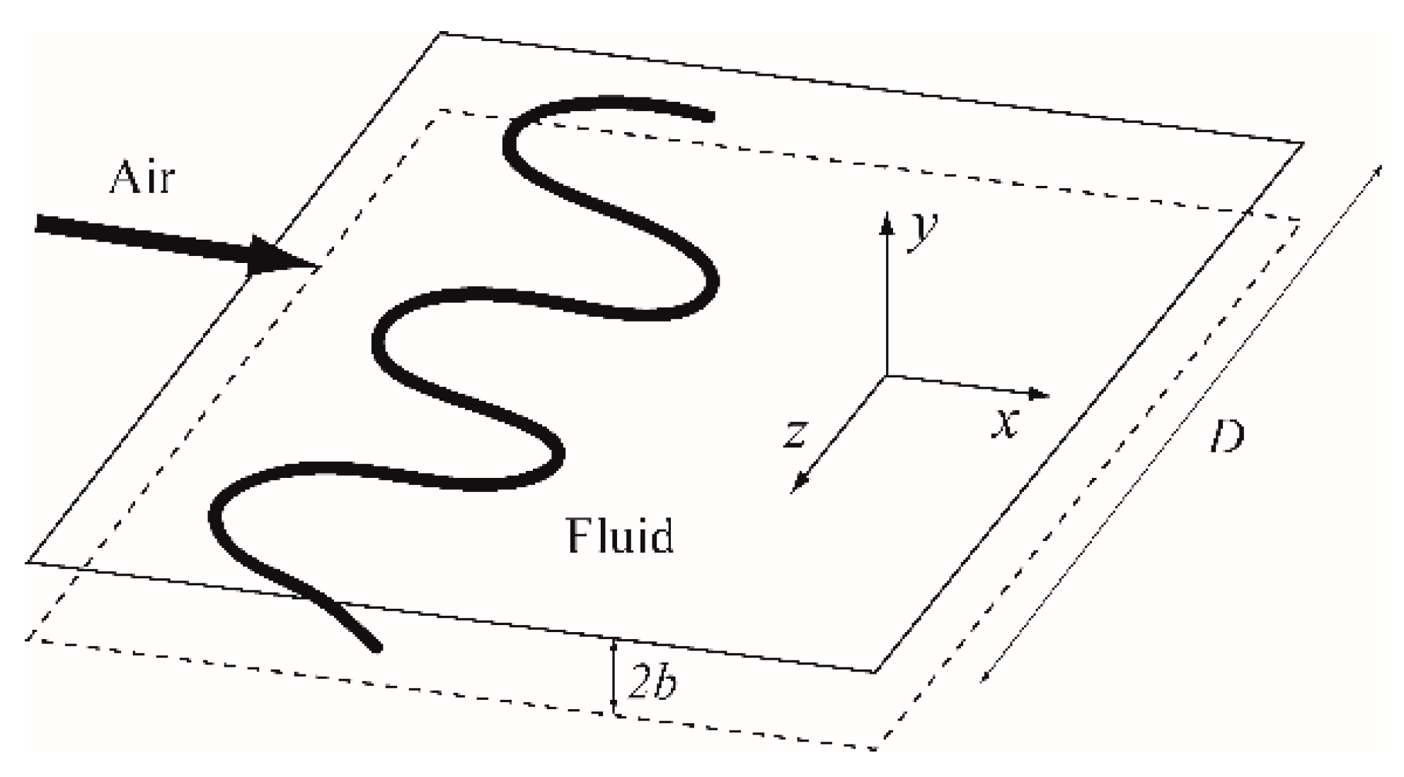
We consider a yield stress fluid pushed by an inviscid fluid (say, air) so that it tends to flow in a given direction x between two parallel plates separated by a distance h = 2b, with a mean fluid velocity U. The initial interface is assumed to be uniform and straight (along the z direction). A stable flow corresponds to a fluid motion along the x direction, uniform along the z direction. For an unstable flow, this interface does not remain straight (see Figure 2).

The linear stability analysis of this flow [15] relies on several assumptions: (i) the constitutive equation of the fluid can be well represented by a HB behaviour; (ii) the lubrication assumption is valid, i.e., the velocity component perpendicular to the cell plan can be neglected; and (iii) the shear stress at the wall, even around the front of the flow, can be approximated by a value close to the exact one for a stable uniform flow through this cell (see [15]):

$${\tau }_w={\tau }_c\left[1+c{\left(\frac{k{U}^n}{{\tau }_c{b}^n}\right)}^d\right],$$

(2)

where c and d two parameters which depend on n. For example, for n = 1/3, c = 1.93, d = 0.9 [15].

Under these conditions, the linear stability analysis of the flow, for negligible gravity effects, predicts that the unidirectional flow above described is fundamentally unstable as soon as the inviscid fluid pushes the yield stress fluid. Moreover, the wavelength of maximum growth is

$${\lambda }_m=2\pi \sqrt{\frac{3\sigma b}{{\tau }_w}}$$

(3)

in which σ is the surface tension. Note that the Newtonian case is recovered from this approach: by using in Equation (3) the wall stress expression for a stable uniform flow of a Newtonian fluid in such a cell, i.e., τ_w = 3μU/b, we find ${\lambda }_m=2\pi b\sqrt{\sigma /\mu U}$, which is the standard expression found from a complete theoretical analysis in the Newtonian case [2].

From Equation (3), we also deduce that the instability will be apparent only if λ_m < D, where D is the width of the flow. This implies that the flow will be apparently unstable if

$${\tau }_w>\frac{12{\pi }^2\sigma b}{D^2}.$$

(4)

Finally, note that, for a yield stress fluid, τ_w tends to τ_c when $U\to 0$ or, more precisely, τ_w ≈ τ_c when kUⁿ/τ_cbⁿ << 1. Thus, at vanishing velocity, the wavelength tends to a finite value, i.e., ${\lambda }_m=2\pi \sqrt{3\sigma b/{\tau }_c}$. This strongly contrasts with the result of the Saffman–Taylor instability for simple fluids (i.e., without yield stress) for which the wavelength tends to infinity when the velocity tends to zero. Thus, for yield stress fluid, if the front width is sufficiently large, we will see the development of a hydrodynamic instability at vanishing velocity. Note that, more precisely, due to the square root of the stress in the wavelength expression, the approximation above leading to neglect the flow rate dependent term in the stress expression, leads to an approximation to within 10% of the exact value of the wavelength if kUⁿ/τ_cbⁿ is smaller than 0.2.

Moreover, in the case of small front velocity, the stress should slightly overcome the yield stress in the regions with highest velocities and, as a consequence, intuitively, the stress might be smaller than the yield stress in regions with lowest velocities (see further demonstration in [15]). As a consequence, the regions left behind should remain static just after the beginning of the unstable process. As long as the fingers grow, the pressure drop applied to these regions therefore decreases so that they should remain static even after a long time.

3.2. Instability in a Radial Hele–Shaw Flow

We consider now the case of a radial flow, with an inviscid fluid pushing the yield stress fluid towards the center. This assumes that, if the plates remain at the same distance, the YSF for example escapes through a central hole. Using again expression (2) for the wall shear stress (which neglects orthoradial components), a linear stability analysis [15] leads to

$${\lambda }_m=2\pi R{\left(\frac{3\sigma b}{\sigma b+{\tau }_w{R}^2}\right)}^{1/2},$$

(5)

in which R is the radius of the circular interface. Once again, this expression allows for recovering the Newtonian case, ${\lambda }_m=2\pi R/\sqrt{\mu U{R}^2/\sigma b^2+1/3}$ [3], by introducing in Label (5) the expression for the wall shear stress of the stable, and the uniform flow of a Newtonian fluid (see above).

Finally, for a YSF, the criterion for the apparent onset of instability (λ_m < 2πR) is:

$${\tau }_w>\frac{2\sigma b}{R^2}.$$

(6)

The above remarks concerning the finite wavelength at vanishing velocity and the tracks left behind still apply in this case.

3.3. Flow Induced by a Traction Test

We now consider the flow induced by a traction test, in which the material initially forming a cylindrical layer situated between two plates, is then deformed as a result of the relative motion of the two plates away from each other along their common axis. As the distance between the plates increases, since the material remains in contact with the plate, the thickness of the sample increases. As a result, the material tends to gather towards its central axis. Let us consider the ideal case where the sample shape remains cylindrical during this process, i.e., the flow is stable and we neglect the deposits of material along its motion along the plates. In that case, as a result of mass conservation, the mean radial velocity (U) is related to the velocity of separation of the plates (V) through

$$U=\frac{R}{4b}V.$$

(7)

From Label (7), we see that, as soon as the aspect ratio (i.e., R/2b) of the sample is sufficiently large, the radial velocity is much larger than the separation velocity. In that case, the lubrication assumption, i.e., the velocity components parallel to the plates are much larger than the perpendicular ones, is relevant, and we can consider that the flow is similar to that resulting from a pure radial flow between plates at a fixed distance from each other. Obviously, this assumption will start to fail at some point during the process, as the aspect ratio progressively decreases toward smaller values when the plates are moved away from each other. In the following, we will a priori assume that the lubrication assumption is valid, and discuss its possible non-validity as an artefact of the tests.

On the other side, for such a traction test, we can easily estimate the normal force needed to separate the plates under the lubrication assumption for stable and sufficiently slow flows (i.e., kUⁿ/τ_cbⁿ << 1) [28]. In that case, the radial flow along the plate induces a shear stress equal to the material yield stress. The momentum balance applied to the sample volume between R and r assuming no surface tension effect and negligible atmospheric pressure leads to:

$$p(r)=\frac{{\tau }_c}{b}(r-R).$$

(8)

The net normal force exerted onto the plate in that case is then found by integrating the pressure (8) over the surface of contact:

$$F=\frac{2\pi {\tau }_c{R}^3}{3b}.$$

(9)

Equation (9) thus provides an expression for the force applied in the case of slow flows. Since the assumed constitutive equation is continuous, i.e., it predicts a continuous transition from rest to slow flows around the yield stress, Equation (9) also provides an expression for the minimum force to induce some motion for a given separation distance and a given radius.

Note that, for a given volume of material (Ω₀ = 2πR²b), this force may be rewritten as

$$F=\frac{4{\tau }_c{\Omega }_0{}^{3/2}}{3\sqrt{\pi }{h}^{5/2}},$$

(10)

which gives the force variation as a function of the distance (h = 2b) between the plates.

4. Results and Discussion

4.1. General Trends

The typical result of a traction test is the formation of an approximately symmetrical deposit over each solid surface, associated with a tendency to a gathering of the material towards the central axis, as proved by the larger thickness of material towards the central part. Depending on the experimental conditions, the final deposit has different aspects, from a simple conical shape to a fingered structure (see [23]). Since the initial shape is cylindrical, a stable flow would maintain a cylindrical interface. As a consequence, a final fingered structure (see Figure 3) is the hallmark of flow instability.

4.2. Force vs. Distance

The force during such a test strongly decreases with the distance and approximately follows a slope of −2.5 in logarithmic scale (see Figure 4), which tends to confirm the validity of Equation (10). However, we can remark that the force curve is shifted towards smaller values when the initial distance is smaller, in contradiction with the above theory since expression (10) only depends on the sample volume and the current distance. This is explained by the development of fingering, which implies that some significant parts of the material do not flow anymore in the radial direction.

Let us try to take this phenomenon into account. We assume that, during the withdrawal of dR, the fingers well develop so that half the material is left behind as deposited material, while the central flowing region is “plain”, with a current volume Ω. Thus, we have a variation of the current volume of material still in the flowing region as dΩ = πRhdR, since, by definition of this volume: Ω = πR²h, we deduce dΩ/Ω = dR/R and by integration Ω = Ω₀R/R₀ = Ω₀²/πhR₀². We finally find $F_c=\frac{2{\tau }_c{\Omega }_0{}^{3/2}}{3{\pi }^{1/2}}{h}_0{}^{3/2}{h}^{-4}$. Although this expression now effectively predicts a decrease of the force with the initial distance, it also predicts a decrease of this force with the current distance as a power −4, in contradiction with the data. Thus, we can conclude that, although we are able to reproduce some qualitative trends through different approaches, we still lack a full theory for describing the force evolution with distance when fingering develops significantly.

4.3. Characteristics of the Instability

4.3.1. Instability Criterion

We now discuss the characteristics of this instability. In order to better discuss the origin of the evolution of the final shape of the deposit with the material and process parameters, we consider the theoretical prediction of the instability criterion (i.e., Equation (6)) under negligible “additional viscous effects”. Note that we checked that for all the tests with the emulsions kUⁿ/τ_cbⁿ was smaller than 0.2, which means that the above simplified expression for the finger width is relevant. This was not the case for the Carbopol gel, for which kUⁿ/τ_cbⁿ was as large as 0.5 at the beginning of the test in some cases, but, in the following, we neglect this aspect and it appears that this does not affect the consistency of our results and analysis. In the instability criterion (Equation (6)), we can then use the approximation τ_w ≈ τ_c, so that this criterion may be rewritten as τ_cΩ₀/h² > 2πσ. From this expression, we see that, if it is to occur, the instability will occur at the beginning of the withdrawal, when the height is the smallest. As a consequence, the instability criterion writes: X = τ_cΩ₀/h₀² > 2πσ. Under these conditions, we can expect that the instability will be “more developed” for increasing values of X.

In Figure 5, we show the different final shapes observed for different values of X as a function of the initial distance between plates. We see that h₀ does not determine solely the intensity of the instability: various deposit aspects are found for a given h₀ value. On the contrary, as expected from the theory, the aspect of the deposits seems to be close for a given value of X: we get approximately similar branched structures along each horizontal line in this representation (see Figure 5). Then, we can determine the limit between the unstable and stable regimes, by considering that the absence of apparent fingering is the hallmark of stable flows. Note that, for small values of h₀, this is an extrapolation, since we were unable to get experimental data in this region of the graph as it required too small sample volumes. We thus find that this limit corresponds to X ≈ 10 Pa·m. (Note that a similar approach from the data of Barral et al. [15] would lead to X ≈ 80 Pa·m.) On the other side, using for the surface tension the value of the interstitial liquid (water) [29], i.e., σ = 0.07 Pa·m, the left hand-side of the instability criterion (6), i.e., 2πσ is equal to 0.4 Pa·m. Thus, we find that experiments give stable flows in a wide range where unstable flows are expected from theory, namely between say X ≈ 10 Pa·m and X ≈ 0.4 Pa·m.

At first glance, this result may be seen as a strong discrepancy between experiments and theory. Actually, this is not so obvious. Indeed, looking at the flows considered as “stable”, we see that they correspond to a rather limited radial flow. Under such conditions, the STI, or more precisely fingering, would simply not have enough time or distance to develop. More precisely, this is the validity of the lubrication assumption, which should be discussed, as we expect that, if this assumption is valid, during the traction test the distance will now increase to large values, i.e., at least of the same order as the initial radius, which implies a significant radial flow. If we compute the ratio h₀/R₀, we find that the stable flows correspond exactly to those for which h₀/R₀ is larger than 0.1. This suggests that here we in fact find stable flows because the lubrication assumption is not valid. In that case, we have indeed a more complex flow than assumed in the theory, in particular there is now likely a significant component of elongation along the vertical axis, which might dampen the instability. In fact, looking further at the initial and final sample shape, we see that the material essentially transforms from a circular disk layer to a cone of same basis, and does not significantly flow radially. Actually, in similar experiments carried out with smooth plates, with roughness of less than one nanometer, no instability at all is observed in a wide range of initial distances [30]. In that case, we have a pure elongation flow along most of the flow. This further confirms the above suggestion that, when the elongational component is significant, no instability can be expected.

This suggests that we cannot really test the validity of the instability criterion because well before the range for which stability is expected, the lubrication assumption is not valid. We can just say that, under the proper assumptions, i.e., lubrication assumption, the flow is unstable, in agreement with the theoretical criterion.

4.3.2. Fingering Wavelength

Let us now try another approach to test the theory, by looking at the wavelength of the fingering. With that aim, we need to look at the fingering characteristics at the onset of the instability, since this is the only aspect relevant within the frame of a linear stability analysis, which considers the flow evolution for a slight perturbation of the initial stable flow. We assume that the corresponding wavelength corresponds to the fingers apparent at the periphery of the initial sample layer and we simply count the number of deposited fingers around the sample, which corresponds to N/2. The theoretical prediction for the finger number N at the onset of the instability, i.e., 2πR/λ_m, as deduced from Label (5) is:

$$N=\frac{1}{\sqrt{3}}{\left(1+\frac{2Y}{\pi }\right)}^{1/2}$$

(11)

in which Y = X/σ.

All the data are shown in Figure 6, where we can see that globally the theoretical prediction is in agreement with the experiments: all the data for the different fluids, different initial distances, and different sample volumes, fall along a master curve which corresponds to an increase of the finger number following on average the theoretical curve. Nevertheless, we can note some discrepancy: at low Y values, the finger number is systematically below (by a factor about 1.5) the theoretical prediction, which suggests that, in that case, the elongational component of the flow plays some significant role and slightly dampens the instability; at large Y, the finger number is slightly above the theoretical prediction, but we have no explanation for that.

5. Conclusions

We have shown that it is in fact not possible to test the theoretical criterion for the instability onset of yield stress fluids in traction tests: as soon as the radial flow induced is sufficiently developed, an unstable flow is expected and effectively observed. On the contrary, in agreement with the theoretical prediction for the finger size appears, i.e., a master curve is obtained when plotting N as a function of X for the different volumes, yield stresses and initial thicknesses in rather large ranges. However, there remains a discrepancy between theory and experiments: the finger number is smaller by a factor about 1.5 for X < 25 Pa·m, and larger by a factor about 1.5 for X > 25 Pa·m. As a consequence, the basic theory can be used to estimate and predict the fingering aspect for any application, as soon as one knows the material yield stress, sample volume and initial thickness. On the other side, this traction test could be used for the estimation of the material yield stress, from an analysis of the fingering characteristics. Further work in that field could focus on the exact flow characteristics during such a traction test, in particular when the instability has begun.

References

- Saffman, P.G.; Taylor, G. The penetration of a fluid into a porous medium or Hele-Shaw cell containing a more viscous liquid. Proc. R. Soc. Lond. 1958, A245, 312–329. [Google Scholar]
- Homsy, G.M. Viscous fingering in porous media. Ann. Rev. Fluid Mech. 1987, 19, 271–311. [Google Scholar] [CrossRef]
- Paterson, L. Radial fingering in a Hele-Shaw cell. J. Fluid Mech. 1981, 113, 513–529. [Google Scholar] [CrossRef]
- Van Damme, H.; Lemaire, E.; Abdelhaye, O.M.; Mourchid, A.; Levitz, P. Pattern formation in particulate complex fluids: A guided tour. In Non-Linearity and Breakdown in Soft Condensed Matter; Bardan, K.K., Chakrabarti, B.K., Hansen, A., Eds.; Lecture Notes in Physics; Springer: Berlin/Heidelberg, Germany, 1994; Volume 437. [Google Scholar]
- McCloud, K.V.; Maher, J.V. Experimental perturbations to Saffman-Taylor flow. Phys. Rep. 1995, 260, 139–185. [Google Scholar] [CrossRef]
- Nittmann, J.; Daccord, G.; Stanley, E. Fractal growth of viscous fingers: Quantitative characterization of a fluid instability phenomenon. Nature 1985, 314, 141–144. [Google Scholar] [CrossRef]
- Lemaire, E.; Levitz, P.; Daccord, G.; Van Damme, H. From viscous fingering to viscoelatic fracturing in colloidal fluids. Phys. Rev. Lett. 1991, 67, 2009–2012. [Google Scholar] [CrossRef]
- Foyart, G.; Ramos, L.; Mora, S.; Ligoure, C. The fingering to fracturing transition in a transient gel. Soft Matter 2013, 32, 7775–7779. [Google Scholar] [CrossRef]
- Wilson, S.D.R. The Saffman-Taylor problem for a non-Newtonian liquid. J. Fluid Mech. 1990, 220, 413–425. [Google Scholar] [CrossRef]
- Sader, J.E.; Chan, D.Y.C.; Hughes, B.D. Non-Newtonian effects on immiscible viscous fingering in a radial Hele-Shaw cell. Phys. Rev. E 1994, 49, 420–432. [Google Scholar] [CrossRef]
- Kondic, L.; Palffy-Muhoray, P.; Shelley, M.J. Models for non-Newtonian Hele-Shaw flow. Phys. Rev. E 1996, 54, R4536–R4539. [Google Scholar] [CrossRef]
- Lindner, A.; Bonn, D.; Meunier, J. Viscous fingering in a shear-thinning fluid. Phys. Fluids 2000, 12, 256–261. [Google Scholar] [CrossRef]
- Lindner, A.; Bonn, D.; Poire, E.C.; Ben Amar, M.; Meunier, J. Viscous fingering in non-Newtonian fluids. J. Fluid Mech. 2002, 469, 237–256. [Google Scholar] [CrossRef]
- Coussot, P. Yield stress fluid flows: A review of experimental data. J. Non-Newton. Fluid Mech. 2014, 211, 31–49. [Google Scholar] [CrossRef]
- Coussot, P. Saffman-Taylor instability for yield stress fluids. J. Fluid Mech. 1999, 380, 363–376. [Google Scholar] [CrossRef]
- Fontana, J.V.; Lira, S.A.; Miranda, J.A. Radial viscous fingering in yield stress fluids: Onset of pattern formation. Phys. Rev. E 2013, 87, 013016. [Google Scholar] [CrossRef] [PubMed]
- Ebrahimi, B.; Mostaghimi, P.; Gholamian, H.; Sadeghy, K. Viscous fingering in yield stress fluids: A numerical study. J. Eng. Math. 2016, 97, 161–176. [Google Scholar] [CrossRef]
- Ebrahimi, B.; Seyed-Mohammad, T.; Sadeghy, K. Two-phase viscous fingering of immiscible thixotropic fluids: A numerical study. J. Non-Newton. Fluid Mech. 2015, 218, 40–52. [Google Scholar] [CrossRef]
- Maleki-Jirsaraei, N.; Lindner, A.; Rouhani, S.; Bonn, D. Saffman-Taylor instability in yield stress fluids. J. Phys. Cond. Matter 2005, 17, S1219–S1228. [Google Scholar] [CrossRef]
- Eslamin, A.; Taghavi, S.M. Viscous fingering regimes in elasto-visco-plastic fluids. J. Non-Newton. Fluid Mech. 2017, 243, 79–94. [Google Scholar] [CrossRef]
- Maleki-Jirsaraei, N.; Erfani, M.; Ghane-Golmohamadi, F.; Ghane-Motlagh, R. Viscous fingering in laponite and mud. J. Test. Eval. 2015, 43, 11–17. [Google Scholar] [CrossRef]
- Lindner, A.; Bonn, D.; Coussot, P. Viscous fingering in a yield stress fluid. Phys. Rev. Lett. 2000, 85, 314–317. [Google Scholar] [CrossRef]
- Barral, Q.; Ovarlez, G.; Chateau, X.; Boujlel, J.; Rabideau, B.D.; Coussot, P. Adhesion of yield stress fluids. Soft Matter 2010, 6, 1343–1351. [Google Scholar] [CrossRef]
- Piau, J.M. Carbopol gels: Elastoviscoplastic and slippery glasses made of individual swollen sponges Meso- and macroscopic properties, constitutive equations and scaling laws. J. Non-Newton. Fluid Mech. 2007, 144, 1–29. [Google Scholar] [CrossRef]
- Coussot, P.; Tocquer, L.; Lanos, C.; Ovarlez, G. Macroscopic vs. local rheology of yield stress fluids. J. Non-Newton. Fluid Mech. 2009, 158, 85–90. [Google Scholar] [CrossRef]
- Bataille, J. Stabilité d’un déplacement radial non miscible. Rev. Inst. Français Pétr. 1968, XXIII, 1349–1364. [Google Scholar]
- Wilson, S.D.R. A note on the measurement of dynamic contact angles. J. Colloid Interface Sci. 1975, 51, 532–534. [Google Scholar] [CrossRef]
- Coussot, P. Rheometry of Pastes, Suspensions and Granular Materials; Wiley: New York, NY, USA, 2005. [Google Scholar]
- Boujlel, J.; Coussot, P. Measuring the surface tension of yield stress fluids. Soft Matter 2013, 9, 5898–5908. [Google Scholar] [CrossRef]
- Zhang, X.; Fadoul, O.; Lorenceau, E.; Coussot, P. Yielding and flow of soft-jammed systems in elongation. Phys. Rev. Lett. 2018, 120, 048001. [Google Scholar] [CrossRef] [PubMed]
Figure 1.
Typical flow curve of a one of our emulsion and of the Carbopol gel. The continuous lines are the Herschel–Bulkley model fitted to data with the parameters: (emulsion emulsion (78%)) τc = 30 Pa, k = 4.5 Pa·sn and n = 0.45; (Carbopol) τc = 70 Pa, k = 23.5 Pa·sn and n = 0.4.
Figure 2.
Scheme of main flow characteristics in a Hele–Shaw cell for a destabilized interface (thick line).
Figure 3.
Fingering aspect of the remaining deposit of yield stress fluid after separation of two plates initially squeezing a thin fluid layer. (Photo Q. Barral).
Figure 4.
Force vs. distance during a traction experiment for an emulsion (82%) (yield stress of 40 Pa) for different initial aspect ratios (corresponding to first point of curves on the left) (Ω = 3 mL). The dashed line is the lubrication model (see text).
Figure 5.
Final aspects of the deposit after plate separation as a function of the parameter X and the initial thickness, for a 40 Pa yield stress emulsion and different sample volumes (the volume corresponding to each picture may be estimated from the value of X and h0 through Ω0 = Xh02/τc). The diameter of the dark disk in all the photos is 10 cm.
Figure 6.
Saffman instability during traction tests with emulsions of various yield stresses, for various sample volumes and various initial thicknesses: Number of fingers as a function of the parameter Y. Caption: emulsions, except when mentioned (Carbopol).
© 2019 by the authors. Licensee MDPI, Basel, Switzerland. This article is an open access article distributed under the terms and conditions of the Creative Commons Attribution (CC BY) license (http://creativecommons.org/licenses/by/4.0/).
Share and Cite
MDPI and ACS Style
Fadoul, O.A.; Coussot, P. Saffman–Taylor Instability in Yield Stress Fluids: Theory–Experiment Comparison. Fluids 2019, 4, 53. https://doi.org/10.3390/fluids4010053
AMA Style
Fadoul OA, Coussot P. Saffman–Taylor Instability in Yield Stress Fluids: Theory–Experiment Comparison. Fluids. 2019; 4(1):53. https://doi.org/10.3390/fluids4010053
Chicago/Turabian StyleFadoul, Oumar Abdoulaye, and Philippe Coussot. 2019. "Saffman–Taylor Instability in Yield Stress Fluids: Theory–Experiment Comparison" Fluids 4, no. 1: 53. https://doi.org/10.3390/fluids4010053