Thermomagnetic Convection of Paramagnetic Gas in an Enclosure under No Gravity Condition


1
School of Mechanical Engineering, Lanzhou Jiaotong University, Lanzhou 730070, China
2
Department of Aeronautics and Astronautics, Tokyo Metropolitan University, Tokyo 191-0065, Japan
3
Grain Inspection Detachment, Lanzhou Grain Bureau, Lanzhou 730030, China
*
Author to whom correspondence should be addressed.
Fluids 2019, 4(1), 49; https://doi.org/10.3390/fluids4010049
Submission received: 13 December 2018
/
Revised: 4 March 2019
/
Accepted: 10 March 2019
/
Published: 15 March 2019
(This article belongs to the Special Issue Numerical Analysis of Magnetohydrodynamic Flows)
Abstract
:The thermomagnetic convection of paramagnetic gaseous oxygen in an enclosure under a magnetic field was numerically studied to simulate the thermomagnetic convection in a space environment with no gravity. The magnetic field in the enclosure was non-uniform and was generated by a permanent magnet which had a high magnetic energy product. The magnet was placed at different locations along one of the adiabatic walls with magnetic poles perpendicular to the hot and cold walls of the enclosure. The heat transfer performance, flow field, and temperature field were studied with each location of the magnet. The results show that the thermomagnetic convection in the enclosure was obviously affected by the location of the magnet. There was an optimum magnet location in terms of the best heat transfer performance in the enclosure. The optimum magnet location changed slightly and moved toward the hot wall as the magnetic flux density increased. The value of the Nusselt number, defined as the ratio of convection to conduction, reached up to 2.54 in the studied range of parameters. By optimizing the magnet location, the convection was enhanced by up to 77% at the optimum magnet location.
1. Introduction
Natural convection plays an important role in energy transportation in an enclosure and has been widely studied due to its significant practical applications [1], such as electric equipment cooling, solar energy collection [2], melting and solidification [3], and thermal convection in spacecraft [4]. As the magnetic field can exert a body force on the magnetic fluid, it is possible to control the fluid motion by using a magnetic field [5]. Krakov and Nikiforov [6,7] numerically demonstrated that heat transfer inside an enclosure can be enhanced by increasing the uniform magnetic field. Tangthieng et al. [8] reported an enhancement of the Nusselt number as high as 45% by applying a permanent magnet on the top of the studied square enclosure. Yu et al. [9] and Tagawa et al. [10] reported that the thermomagnetic convection in a rectangular cavity was obviously affected by the direction of the magnetic field. Vatani et al. [11] studied the thermomagnetic convection of a ferrofluid flow induced by the internal magnetic field around a vertical current-carrying wire and found that increasing the current increased the Nusselt number nonlinearly, ultimately enhancing the heat transfer capability of the induced ferrofluid flow. Vatani et al. [12] experimentally investigated the thermomagnetic convection in ferrofluid in a vertical transient hot-wire cell. They observed that thermomagnetic convection in ferrofluid occurs earlier than natural convection in non-magnetic fluids for similar experimental conditions, and that the onset of thermomagnetic convection was dependent on the current supplied to the wire. Jiang et al. [13] numerically investigated the effect of permanent magnetic quadrupole fields on the thermomagnetic convection of air in a porous square enclosure in the presence or absence of a gravity field. Two cellular structures with horizontal symmetry about the middle plane of the enclosure were observed. In addition, the Nusselt number was increased with the increase of the magnetic force number under non-gravitational conditions. Yang et al. [14] also pointed out that the centrifugal-form magnetic force exhibits different flow and heat transfer characteristics from the gravitational free convection. Song et al. [15] numerically studied the effects of magnet position and magnet strength on the thermomagnetic convection in a square enclosure under combined magnetic and gravitational fields. The Nusselt number increased with the increase of magnetic flux density when the magnet was located near a hot wall. The optimum position of a magnet for the best heat transfer is reported. Ashouri et al. [16] numerically studied the pure magnetic convection ferrofluid flow in a square cavity under the magnetic field supplied by a permanent magnet below the bottom wall of the square cavity. Results show that the convective flow and heat transfer rise, increasing with the strengthening of the magnetic field in the absence of a gravity field. Szabo and Früh [17] numerically studied the transition from natural convection to thermomagnetic convection of a magnetic fluid in a non-uniform magnetic field. Their results show that the transition from a single buoyancy-driven convection cell to a single thermomagnetically driven cell is via a two-cell structure, and that the local effect on the flow field leads to a global effect on the heat transfer with a minimum of the Nusselt number in the transition region.
From the above mentioned review we found that most of the published papers focus on the effect of magnetic field direction or the inclined angle of a magnetic field on thermal convection. The thermomagnetic convection in the pure non-uniform magnetic field without a gravity field, such as the requirement in astronautics engineering, has scarcely been studied. The effect of the magnetic field, especially the non-uniform magnetic field supplied by a permanent magnet on thermomagnetic convection is still not well illustrated in the literature. In this paper, the thermomagnetic convection of paramagnetic gaseous oxygen under a pure non-uniform magnetic field supplied by a permanent magnet with magnetic poles paralleling to the adiabatic walls was numerically studied. The location of the magnet was optimized in terms of the strongest thermomagnetic convection in the enclosure.
2. Physical Model
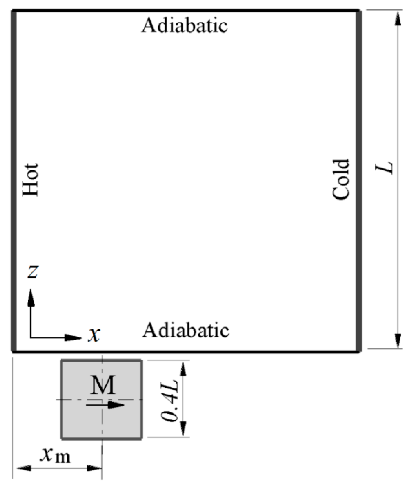
The studied physical model is shown schematically in Figure 1. The left wall of the square enclosure was kept at a constant high temperature and named the hot wall. Meanwhile, the right wall of the square enclosure was kept at a constant low temperature and named the cold wall. The other walls, that is, the horizontal walls, were adiabatic. The permanent magnet, the Neodymium-Iron-Boron, which possesses a high residual magnetic flux density, was placed aside the bottom wall, with the middle plane overlapping the square enclosure. The magnet was assumed to be uniformly magnetized in an x-direction, with the magnetic poles parallel to the bottom wall of the enclosure. The length of the square enclosure was L = 0.05 m. The length of the permanent magnet was set to 0.4 L. The gap between the magnet and the enclosure was δ = 0.04 L. The distance of the magnet from the hot wall was changeable along the bottom wall of the enclosure. The distance between the center of the magnet and the hot wall of the enclosure ranged between xm/L = 0.0 and 1.0. Gaseous oxygen, which has a high mass magnetic susceptibility, was considered to be the working medium in the enclosure. The details of the physical properties of gaseous oxygen and other parameters are summarized in Table 1. The residual magnetic flux density changed from 0.5 Tesla to 3.0 Tesla with an interval of 0.5 Tesla. There were a total of 78 cases with different magnet flux densities and different magnet locations.
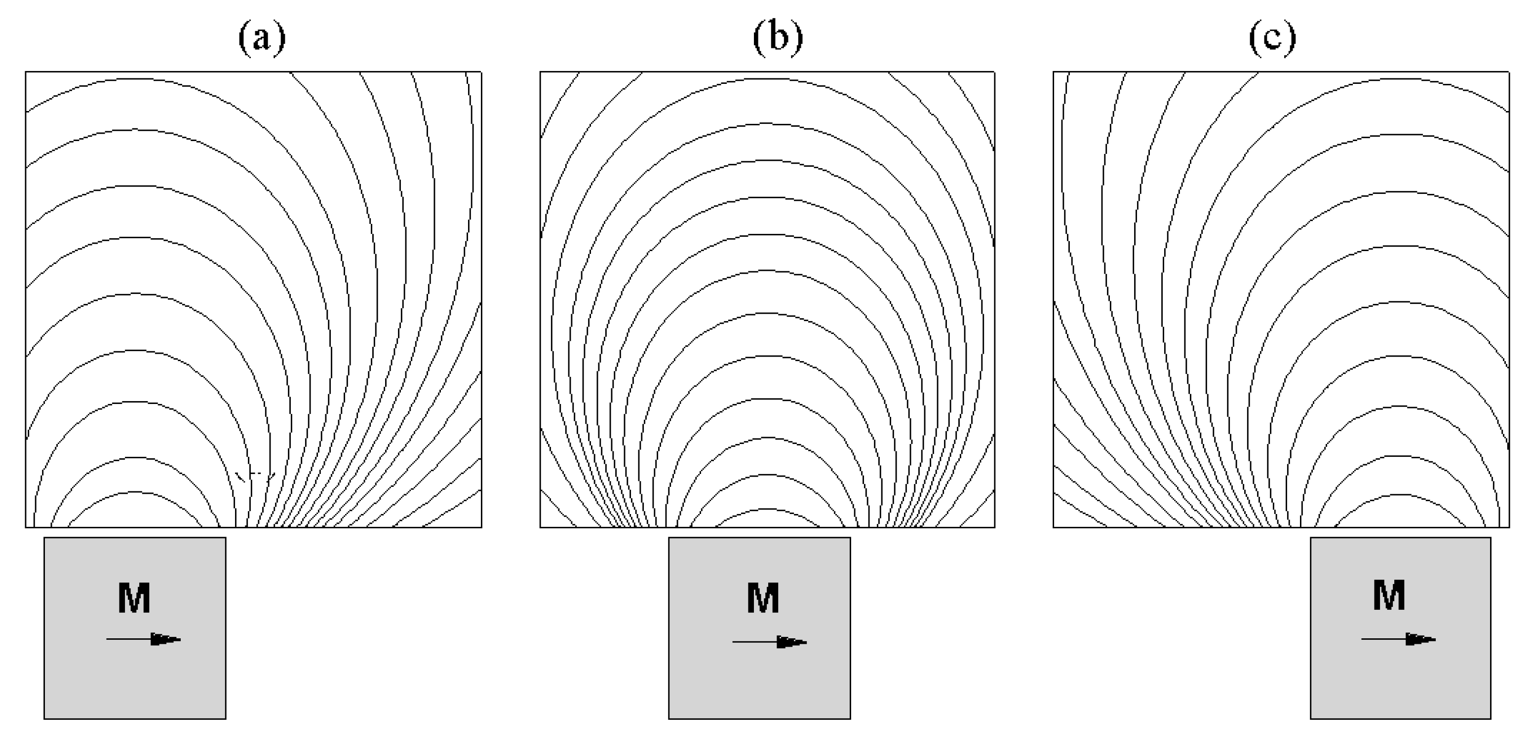
The magnetic field lines in the enclosure are shown in Figure 2 for different positions of the magnet. The magnets were placed at xm/L = 0.2, 0.5, and 0.8 for Figure 2a–c, respectively. The magnetic fields in the enclosure were quite different depending on the positions of the magnet. Thus, it is valuable to study the thermomagnetic convection inside the enclosure for different magnet positions with the poles of the magnet paralleling to bottom wall of the enclosure.
3. Mathematical Equations
The magnetizing force, which is similar to the gravitational force, is a conservative force. Thus, both magnetic field gradient and the temperature gradient are necessary for thermomagnetic convection. The normal expression of magnetizing force is as follows [15,18]:
The magnetic induction B can be expressed as
where A is the vector potential generated by the permanent magnet at the calculated point. The calculation of magnetic induction B refers to Reference [15].
The momentum equation including the magnetizing force is as follows:
The gas is assumed as an incompressible Newtonian fluid, and the Boussinesq approximation that density is assumed to be constant except for the density difference for buoyancy force was employed. The parameters under the isothermal state are marked ρ0, p0, and χ0 at reference temperature T0.
When there is a temperature difference, the magnetic susceptibility and density also change with temperature. Subtracting Equation (4) from Equation (3), we get
The density can be expressed by a Taylor expansion around a reference state T0 as follows:
On the other hand, the thermal volume coefficient of expansion β for gas is
Then Equation (6) can be rewritten as follows by keeping only two terms of the Taylor expansion:
With the ideal gas law, Equation (7) can be rewritten as
Using the Taylor expansion around a reference state T0, the difference of ρχ can be written as
The magnetic susceptibility of paramagnetic gas is a function of temperature according to the Curie law,
Equation (10) can be rewritten as
Therefore, the momentum equation, Equation (5), can be written as follows:
The continuity equation is
The energy equation is
The temperature of the cold wall is selected as the reference temperature, T0 = Tc. The initial conditions for the gas in the enclosure are u = w = 0, and T = T0, and no-slip conditions are applied on the walls of the enclosure.
The dimensionless parameters used are Nusselt numbers on the hot and cold walls. Local Nusselt number Nuh and Nuc on the hot and cold walls are as follows:
The averaged Nusselt number is obtained by averaging Nuh on the hot wall,
4. Grid Dependence and Validation
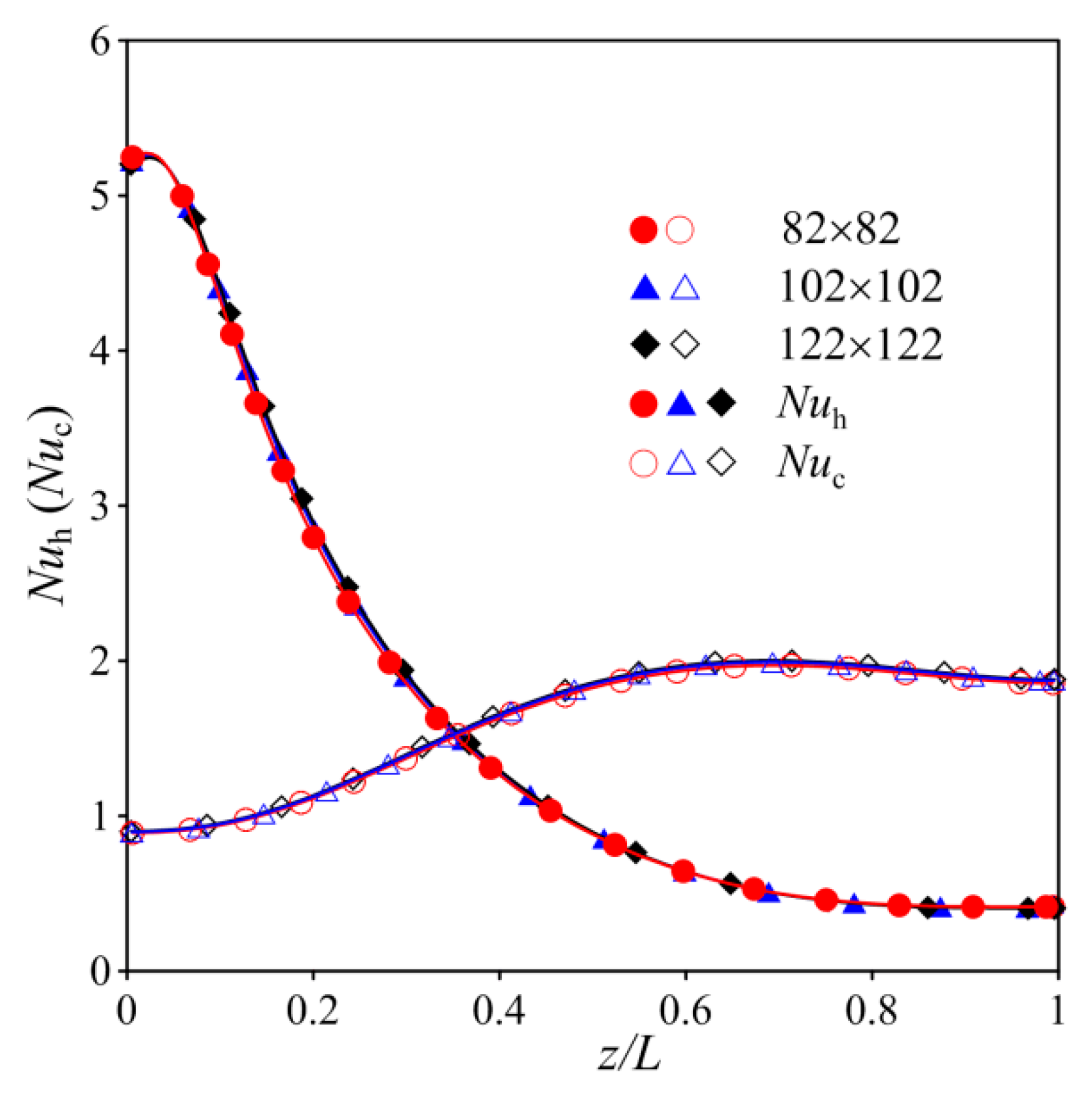
The grid dependence study was carried out between three grid systems 82 × 82, 102 × 102 and 122 × 122. The magnet was located at xm/L = 0.0 with Br = 2.0 T. The fine grid was about 2.2 times larger than the coarse grid. The distributions of Nuh on the hot wall and Nuc on the cold wall for different grid systems are presented in Figure 3. As the magnetic field was non-uniform, the distribution of Nuh on the hot wall was quite different from Nuc on the cold wall, which was also quite different from the distributions of Nuh and Nuc under a gravity field, as reported in Reference [13]. The results of local Nu on both hot and cold walls are nearly the same for the three different grid systems studied. Thus, the results are grid independent in a large range of grid numbers and the medium-size grid system, 102 × 102, was selected for all computations in order to save computation resources.
In order to validate the numerical method, the natural convection in a square enclosure filled with air, reported by De Vahl Davis [19], was tested and compared with the reported results. The comparisons of the average values of Nu on the hot wall are shown in Table 2. The averaged Nusselt number agrees well with the results reported by De Vahl Davis [19]. The maximum difference was less than 0.05%.
5. Results and Discussion
5.1. Effect of Location of Magnet on Temperature
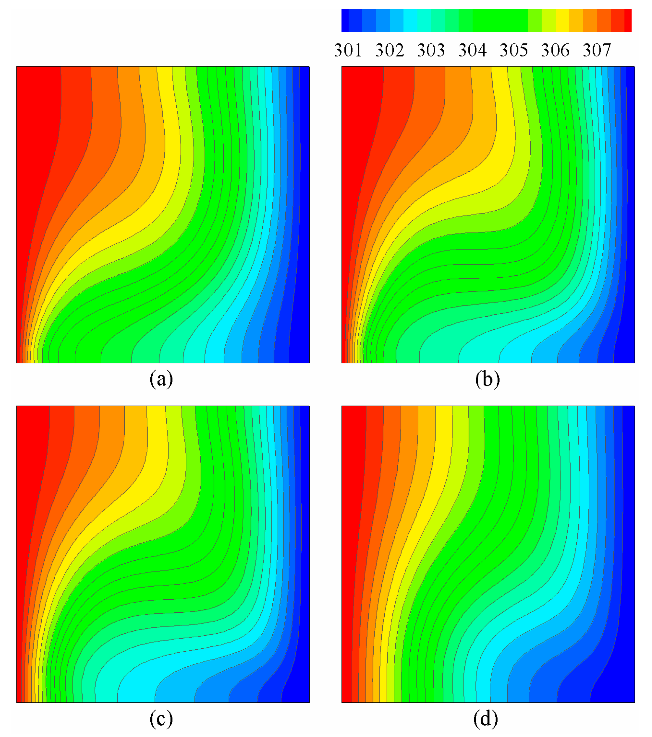
The distributions of temperature in the enclosure with different magnet locations are shown in Figure 4 for Br = 2.0 T. The magnet locations in Figure 4a–d are xm/L = 0.2, 0.4. 0.6 and 1.0, respectively. As the magnetic field depends on the location of the magnet, the temperature fields for different magnet locations were quite different from each other. The temperature near the hot wall increased quickly from the bottom to the top of the enclosure and a large temperature gradient existed near the lower part of the hot wall. As the fluid washed toward the hot wall near the bottom wall, the temperature layer was thin near the lower part of the hot wall. The temperature near the upper part of the hot wall was high due to the strong convection near the lower part of the hot wall. Comparing Figure 4b with Figure 4a, the temperature gradient near the lower part of the hot wall in Figure 5b is slightly larger than that in Figure 4a. When the magnet location changed from xm/L = 0.4 to 1.0, the temperature gradient near the lower part of the hot wall decreased while the temperature gradient near the upper part of the hot wall increased, meaning the heat transfer on the lower part of the hot wall decreased and the heat transfer on the upper part of the hot wall increased. When the magnet was fixed at xm/L = 1.0, as shown in Figure 4d, the temperature near the hot wall increased gradually and the difference in temperature gradient near the hot wall was small compared with Figure 4a–c, meaning that the heat transfer near the hot wall was quite weak when the magnet was located at xm/L = 1.0.
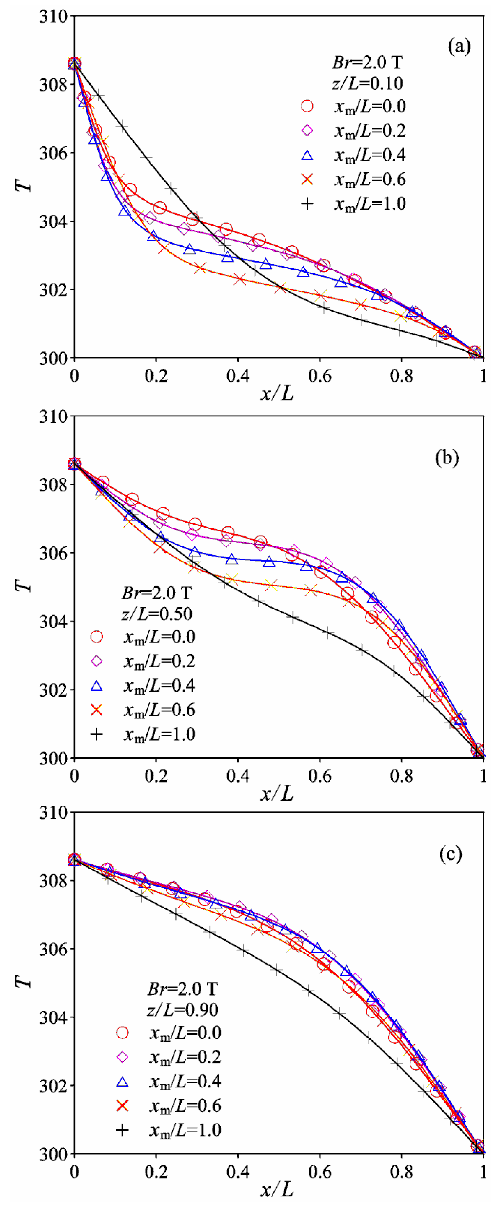
Figure 5 shows the distribution of temperature on the selected lines at z/L = 0.10, 0.50 and 0.90 for different magnet locations. The different locations of the magnet had an obvious effect on the distribution of temperature of the magnetic field. The temperature decreased from the hot wall to the cold wall. On the line at z/L = 0.10 there was large temperature gradient near the hot wall. The temperature decreased quickly in the region with x/L, changing from 0.0 to around 0.2. Then, the value of the temperature decreased gradually until the cold wall. The temperature gradient near the hot wall first increased a little when the location of magnet changed from xm/L = 0.0 to 0.4, then the temperature gradient decreased when the location of magnet changed from xm/L = 0.4 to 1.0. Obvious differences in Nu exist on the line at z/L = 0.10 in the range of x/L between 0.2 and 0.8. On the line at z/L = 0.50, the temperature was higher than that of the line at z/L = 0.10, and the temperature gradient was smaller than that of the line at z/L = 0.10. Meanwhile, the temperature gradient near the cold wall was higher than that of the line at z/L = 0.10. On the line at z/L = 0.90, as shown in Figure 5c, the temperature gradient near the hot wall continued to decrease and the temperature decreased gradually from the hot wall to the cold wall. The temperature gradient near the cold wall was larger than that near the hot wall on the line at z/L = 0.90.
5.2. Effect of Location of Magnet on Flow Field
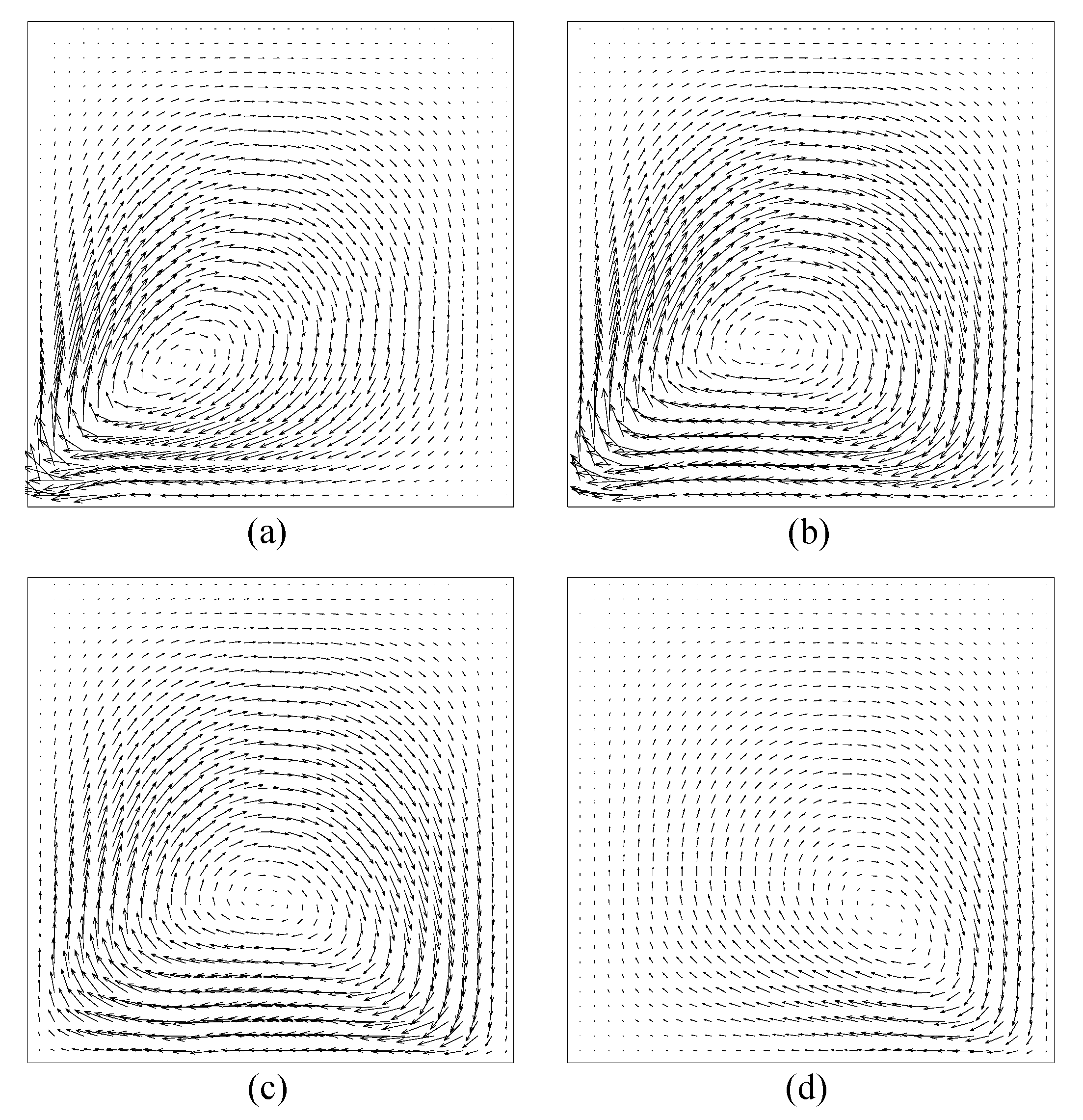
Figure 6 shows the flow field for different locations of the magnet with Br = 2.0 T. The magnet locations for Figure 6a–d were xm/L = 0.2, 0.4, 0.6 and 1.0, respectively. The velocity fields in the square enclosure were quite different from each other for different magnet locations. Large velocities were located in the region where the magnetic field was strong. There was one vortex rotating in a clockwise direction near the bottom wall of the enclosure and the vortex moved along with the moving of the magnet locations. The center of the vortex moved from the left to the right of the enclosure when the magnet location moved from left to right. In Figure 6a, the gas with a large velocity flowed along the bottom wall and washed toward the lower part of the hot wall under the driving magnetic force. The vortex increased a little when the magnet location moved from xm/L = 0.2 to xm/L = 0.4, as shown in Figure 6a,b. The vortex moved away from the bottom left corner, and the zone with a large velocity also increased compared with that in Figure 6a. The strength of the vortex also decreased and the center of the vortex kept moving away from the left wall and toward the right wall, along with the magnet location as it changed from xm/L = 0.4 to xm/L = 1.0. When the magnet was placed at xm/L = 1.0 in Figure 6d, the flow field became very weak. Thus, the flow field was obviously affected by the magnet location.
5.3. Effect of Location of Magnet on Buoyancy Force
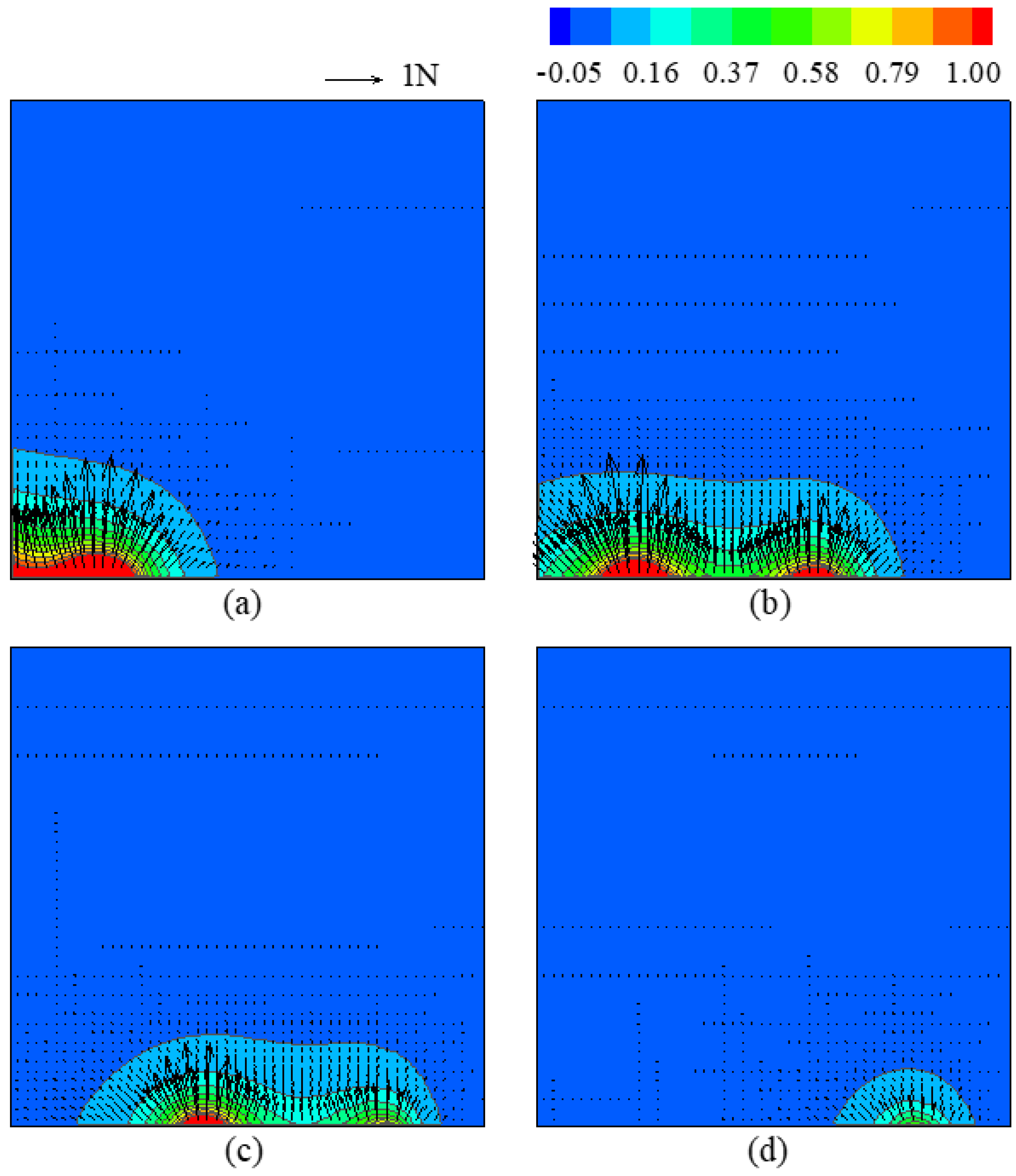
Figure 7 shows the vector plot of F inside the enclosure for different locations of the magnet. The combined contour plot relates to the buoyancy force Fz. As the magnetic field decreased quickly in the short distance from the magnet surface, there was a large value F only in a small region around the magnet. As the magnetic buoyancy force related to the combination of temperature and magnetic field, the values of F were not symmetric about the z-center-line of the magnet, although the magnetic field was symmetric about the z-center-line of the magnet. The temperature decreased from the hot wall to the cold wall, thus F decreased gradually, along with the magnet moving from the hot wall to the cold wall. The values of F near the left corner of the magnet were obviously larger than that near the right corner of the magnet. The value Fz was positive in the enclosure because the magnet was located below the enclosure. The value Fx was a little complicated. Fx was positive on the right of the magnet and negative on the left of the magnet. Fx was positive between the left pole and z-center-line of the magnet, while it was negative between the z-center-line and the right pole of the magnet.
Figure 8 shows the distribution of buoyancy force Fz on the selected lines with different magnet locations for Br = 2.0 T. The magnetic buoyancy force relates not only to the temperature difference but also tightly to the gradient of the square of magnetic field strength. As there was a large gradient of the square of magnetic field strength near the corners of the magnet, large values of magnetic force Fz were obtained near the corners of the magnet. The distribution line of Fz was wave-like and there are two peak points according to the corners of the magnet. As the magnetic field was symmetric about the z-center-line of the magnet and the temperature generally decreased from the left wall to the right wall, the left peak point of Fz was larger than the right peak point of Fz. On the line at z/L = 0.10, as shown in Figure 8a, the values of Fz near the hot wall increased first when the magnet location changed from xm/L = 0.0 to xm/L = 0.2. Then, the value of Fz near the hot wall decreased generally along with the moving of the magnet from xm/L = 0.2 to xm/L = 1.0. When the left pole of the magnet overlapped with the left wall, that is xm/L = 0.2, the largest value of Fz was obtained near the hot wall because this was the location of the strongest magnetic field near the hot wall, where the temperature was also the highest. Then, the value of Fz decreased quickly along x-direction due to the decrease in both temperature and magnetic field strength. Around the right corner of the magnet, where the magnetic field strength was high, the peak value of Fz was also obtained, although the temperature was low.
When the magnet continued moving away from the hot wall, such as at xm/L = 0.4, the magnetic field became weak near the hot wall and the value of Fz near the hot wall decreased. The position of the peak value of Fz also moved away from the hot wall and the value of Fz decreased due to the decrease in temperature away from the hot wall. Meanwhile the difference in Fz between the two peak values also decreased due to the decrease in the temperature gradient toward the cold wall, as shown in Figure 4. When the magnet was located at xm/L = 1.0, with the cold wall overlapping with the center of the magnet, the magnetic field around the hot wall was very weak and the value of Fz was very small, close to zero. There was only one peak value of Fz near the cold wall corresponding to the strong magnetic field near the left corner of the magnet. On the lines at z/L = 0.50 and 0.90, as shown in Figure 8b,c, the values of Fz were smaller, compared with those shown in Figure 8a, due to the weak magnetic field in the region far away from the bottom of the enclosure. As the magnetic field was weak and the difference in magnetic field strength on the selected lines was quite small, there was a slight effect of corners of the magnet on the values of Fz. Thus, the peak values of Fz related to the corners of the magnet were not obvious at z/L = 0.50 and 0.90. The magnetic buoyancy force Fz was mainly dominated by the temperature on the upper part of the enclosure where the magnetic field was quite weak.
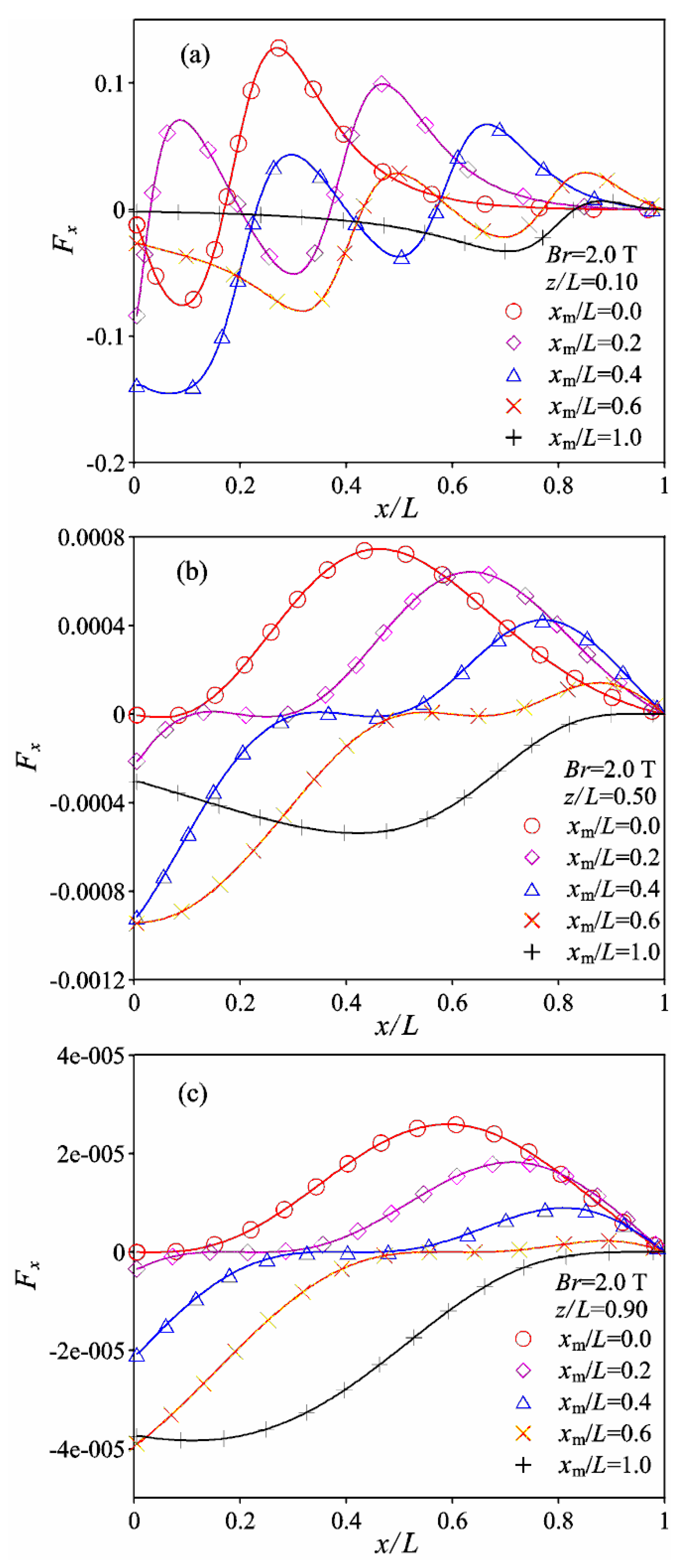
The distributions of Fx on the selected lines located at z/L = 0.10, 0.50 and 0.90 are presented in Figure 9 for different magnet positions. Fx was zero at the point of the intersection of the selected line and the z-center-line of the magnet because of the zero value of the magnetic field gradient along the x-direction at the intersection point. On the line at z/L = 0.1, as shown in Figure 9a, the value of Fx was nearly zero near the hot wall when the magnet was located at xm/L = 0.0. The value of Fx was negative in the region between x/L = 0.0 and 0.20, and Fx was zero at the points ahead of x/L = 0.2, corresponding to the right corner of the magnet. Then, Fx became positive and reached maximum value in the region behind the corner of the magnet. The value of Fx first decreased quickly a short distance away from the pole of the magnet and then decreased gradually until zero on the cold wall. The value of Fx was also nearly zero around the position at x/L = 0.4 when the magnet was located at xm/L = 0.4. In the region between x/L = 0.4 and 1.0, the thermomagnetic convection was affected by the right part of the magnetic field and the distribution of Fx was similar to that of the magnet location at xm/L = 0.4. In the region between x/L = 0.0 and 0.4, the thermomagnetic convection was affected by the left part of the magnetic field. The value Fx was negative in the region between x/L = 0.0 and 0.20, which was on the left of the left pole of the magnet. In the region between x/L = 0.2 and 0.4, Fx was positive and the peak value of Fx was obtained between x/L = 0.2 and 0.4. When the magnet moved from xm/L = 0.0 to xm/L = 1.0, the peak value of Fx, due to the right pole of the magnet and the peak value in accordance with the region between the poles, decreased gradually due to the decrease in temperature. The peak value of Fx, due to the left pole of the magnet, increased first when the magnet moved from xm/L = 0.2 to xm/L = 0.4 and then decreased gradually from xm/L = 0.4 to xm/L = 1.0. There was no peak point related to the left pole of the magnet for the location of the magnet at xm/L = 0.0, because the z-center-line of the magnet overlapped with the hot wall and the thermomagnetic convection in the enclosure was mainly affected by the right part of the magnetic field. On the lines at z/L = 0.5 and 0.9, as shown in Figure 9b,c, the magnetic fields were quite weak and Fx was also quite small compared with that of the line at z/L = 0.1. The value of Fx was positive in the region covered by the right part of the magnetic field, and a negative value of Fx was obtained in the region covered by the left part of the magnetic field.
5.4. Effect of Location of Magnet on Nu
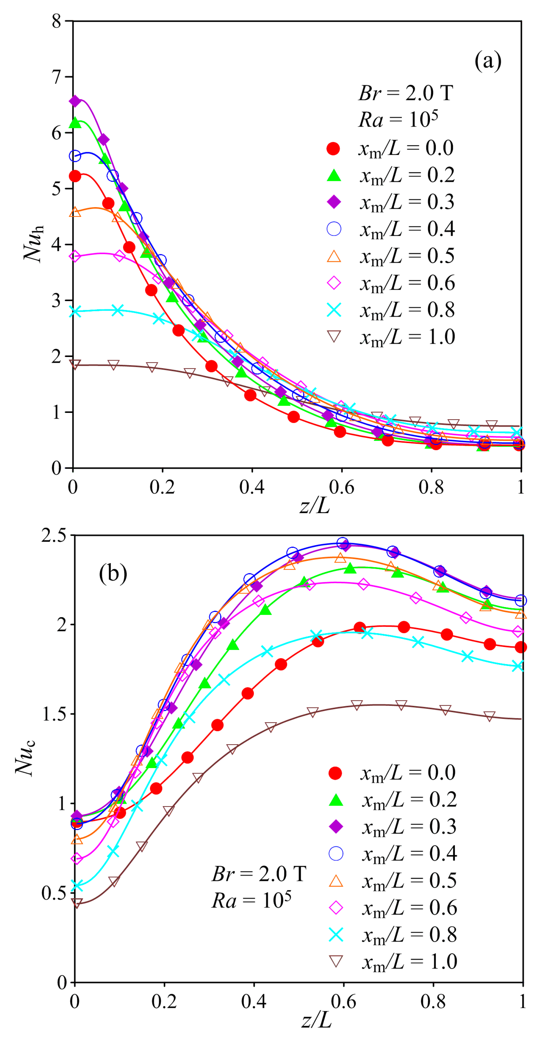
Figure 10 shows the effect of the location of the magnet with Br = 2.0 T on the distribution of Nuh on the hot wall and Nuc on the cold wall. The maximum value of Nuh was obtained near the bottom wall due to the combination of the high strength of magnetic field and temperature. The maximum value of Nuh first increased, with the magnet moving from xm/L = 0.0 to xm/L = 0.3, and got the largest maximum value when the magnet was located at xm/L = 0.3. Then, the maximum value of Nuh for different magnet locations decreased when the magnet moved from xm/L = 0.3 to xm/L = 1.0. The maximum value for the case with xm/L = 0.3 was about 3.6 times larger than that of the case with xm/L = 1.0, and about 43% larger than when the magnet was located at the center with xm/L = 0.5. Nuh decreased along the hot wall due to the increase in temperature and decrease in temperature gradient when the fluid, with high temperature flowing upward the hot wall. Nuh on the upper part of the hot wall generally increased with the increase of the value of xm/L. In addition, the difference in Nuh between cases with different magnet locations was much smaller compared with that on the lower part of the hot wall. The maximum values of Nuc on the cold wall were much smaller than Nuh on the hot wall. The values of Nuc on the upper part of the cold wall were higher than that on the lower part of the cold wall, which was converse to the distribution of Nuh on the hot wall. In the regions of the upper part of the hot wall and the lower part of the cold wall, the values of both Nuh and Nuc were less than 1. The reason is that the temperature gradients, as shown in Figure 5, are quite small in the regions near the upper part of the hot wall and the lower part of the cold wall. Thus, the conduction in the regions with a small temperature gradient was suppressed due to the thermomagnetic convection and the values of Nuh and Nuc were less than 1.
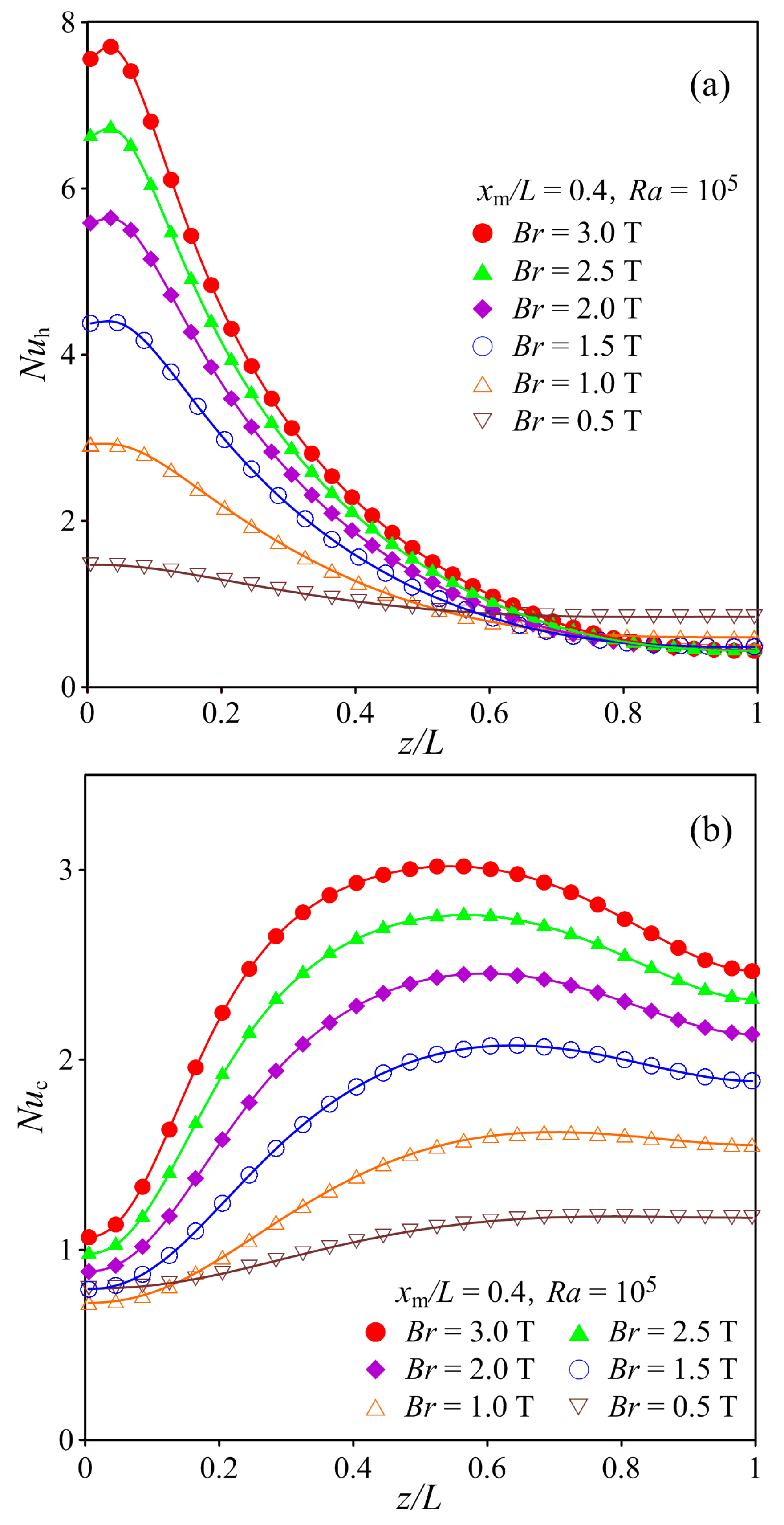
Figure 11 shows the effect of magnet strength on the distributions of Nuh and Nuc on the hot and cold walls when the magnet was located at xm/L = 0.4. In the lower part of the hot wall, Nuh increased with the increase of Br. While in the upper part of the hot wall with z/L > 0.6, the difference in the value of Nuh was slight and the values were nearly the same for Br > 1.0 T. The difference in Nuh on the lower part of the hot wall decreased with the increase of Br. The maximum value of Nuh for Br = 3.0 T was about 5.24 times larger than that for Br = 0.5 T. Nuc increased first away from the bottom and reached its maximum value around the center of the cold wall. Then, Nuc decreased from the maximum value point until the top. The value of Nuc near the top wall was higher than that near the bottom wall. Magnet strength had an obvious effect on the distribution of Nuc, and Nuc generally increased with the increase of Br. In addition, the point with the maximum value of Nuc moved downward with increasing Br. The values of Nuh and Nuc were also less than 1 for some cases with different values of Br in the regions near the upper part of the hot wall and lower part of the cold wall. The reason was the same as that discussed in the figure, that the conduction in these regions was suppressed compared to the pure conduction in the enclosure with magnetic field.
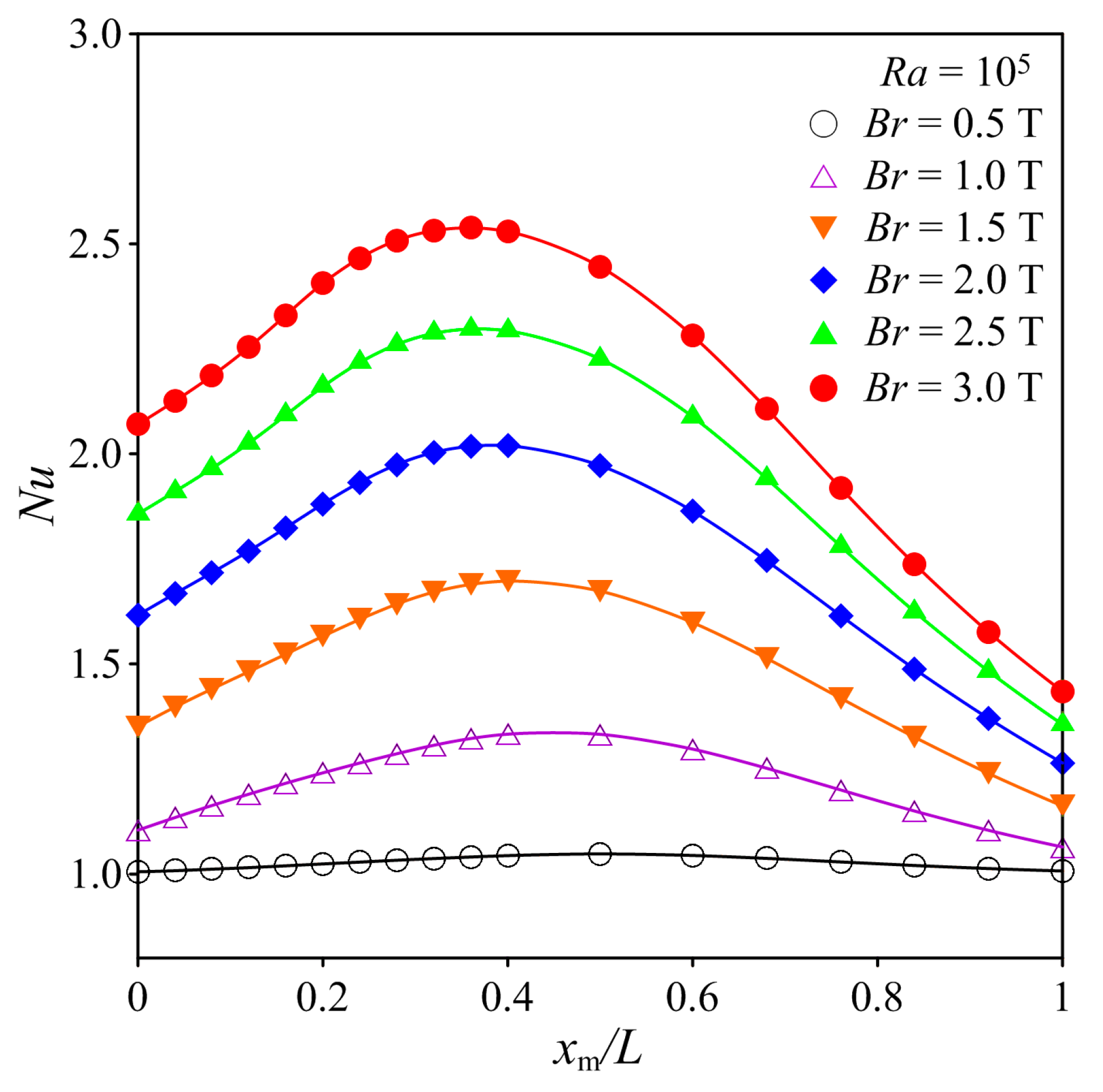
Figure 12 shows the distribution of averaged Nu in the enclosure as a function of the magnet location xm/L and the different residual magnetic flux densities of Br. Nu increased with the increase of residual magnetic flux density. Under the same residual magnetic flux density, Nu first increased and then decreased in the studied range of magnet position between xm/L = 0.0 and1.0. There was an optimum location of the magnet in terms of the largest value of Nu and the optimum locations of the magnet are slightly different from cases with different values of Br. The optimum location of the magnet for the cases with Br = 0.5, 1.0, 1.5, 2.0, 2.5 and 3.0 T were xm/L = 0.5, 0.4, 0.4, 0.4, 0.36 and 0.36, respectively. The optimum location moved slightly toward the hot wall with the increase of Br. The maximum values of Nu at the optimum locations reached up to 2.54, 2.02 and 1.33 for Br = 3.0 T, 2.0 T and 1.0 T, respectively. Compared with the case of xm/L = 1.0, the value of Nu at the optimum location increased by 77.0%, 69.4%, 60.0%, 46.1%, 25.2 and 4.0% for different cases with Br = 3.0 T, 2.5 T, 2.0 T, 1.5 T, 1.0 T and 0.5 T, respectively. Thus, thermomagnetic convection can be further enhanced by optimizing magnet location.
6. Conclusions
Thermomagnetic convection in an enclosure under a non-uniform magnetic field supplied by a permanent magnet at different locations was studied numerically. The permanent magnet was arranged in a novel manner, with the magnet being placed near the adiabatic wall with the poles parallel to the adiabatic wall. The main conclusions can be summarized as follows:
- The location of magnet had a significant effect on the distribution of Nu on the hot wall, especially on the lower part of the hot wall. The maximum local Nu on the hot wall reached up to 2.9, 5.6 and 7.7 for Br = 1.0 T, 2.0 T and 3.0 T, respectively.
- The value of Nu on the upper part of the hot wall and on the lower part of the cold wall was less than 1.0, due to the suppression of conduction with a much lower temperature gradient caused by the thermomagnetic convection.
- The optimum location of the magnet exists in terms of the largest value of Nu. The optimum location of the magnet ranged from xm/L = 0.5 to 0.36, when the magnetic flux density increased from 0.5 T to 3.0 T. Compared with the case of xm/L = 1.0, the average value of Nu in the enclosure could be increased by up to 77% by optimizing the location of the magnet for the studied range of parameters.
Author Contributions
Conceptualization, K.S. and T.T.; Methodology, K.S.; Data Curation, S.W., W.S. and S.Z.; Writing-Original Draft Preparation, K.S.; Writing-Review & Editing, T.T.
Funding
This research was funded by the National Natural Science Foundation of China (51866007), the Gansu Provincial Natural Science Foundation (17JR5RA092) and Collaborative Innovation Team Project (2018C-13), and the Foundation of a hundred youth talents training program of Lanzhou Jiaotong University.
Conflicts of Interest
The authors declare no conflict of interest.
Nomenclature
| A | vector potential (T·m) |
| B | magnetic flux density (T) |
| Br | residual magnetic flux density (T) |
| C | Curie constant (K·m3/kg) |
| c | cold wall |
| cp | specific heat at constant pressure (kJ/(kg·K)) |
| fm | magnetizing force (N/m3) |
| F | magnetic force (N/m3) |
| Fx | magnetic buoyancy force along x-direction (N/m3) |
| Fz | magnetic buoyancy force along z-direction (N/m3) |
| h | hot wall |
| L | length of cavity (m) |
| M | magnetization (A/m) |
| Nu | Nusselt number (-) |
| p | pressure (Pa) |
| Pr | Prandtl number (-) |
| r | unit vector (-) |
| Ra | Rayleigh number (-) |
| Rg | Gas constant (J/(kg·K)) |
| T | temperature (K) |
| u | velocity vector (m/s) |
| v | volume (m3) |
| x, z | coordinate (m) |
| xm | location of magnet |
| α | thermal diffusivity of gas (m2/s) |
| β | volumetric thermal expansion coefficient (1/K) |
| λ | thermal conductivity of oxygen (W/(m·K)) |
| μ | dynamic viscosity (Pa·s) |
| μm | magnetic permeability of free space (H/m) |
| ν | kinematic viscosity (m2/s) |
| ρ | density (kg/m3) |
| χ | mass magnetic susceptibility of oxygen (m3/kg) |
| 0 | reference state |
References
- Das, D.; Roy, M.; Basak, T. Studies on natural convection within enclosures of various (non-square) shapes—A review. Int. J. Heat Mass Transf. 2017, 106, 356–406. [Google Scholar] [CrossRef]
- Joudi, K.A.; Hussein, I.A.; Farhan, A.A. Computational model for a prism shaped storage solar collector with a right triangular cross section. Energy Convers. Manag. 2004, 45, 391–409. [Google Scholar] [CrossRef]
- Kalaiselvam, S.; Veerappan, M.; Aaron, A.A.; Iniyan, S. Experimental and analytical investigation of solidification and melting characteristics of PCMs inside cylindrical encapsulation. Int. J. Therm. Sci. 2008, 47, 858–874. [Google Scholar] [CrossRef]
- Mukhopadhyay, A.; Ganguly, R.; Sen, S.; Puri, I.K. A scaling analysis to characterize thermomagnetic convection. Int. J. Heat Mass Transf. 2005, 48, 3485–3492. [Google Scholar] [CrossRef]
- Bahiraei, M.; Hangi, M. Flow and heat transfer characteristics of magnetic nanofluids: A Review. J. Magn. Magn. Mater. 2015, 374, 125–138. [Google Scholar] [CrossRef]
- Krakov, M.S.; Nikiforov, I.V. To the influence of uniform magnetic field on thermomagnetic convection in square cavity. J. Magn. Magn. Mater. 2002, 252, 209–211. [Google Scholar] [CrossRef]
- Krakov, M.S.; Nikiforov, I.V. Thermomagnetic convection in a porous enclosure in the presence of outer uniform magnetic field. J. Magn. Magn. Mater. 2005, 289, 278–280. [Google Scholar] [CrossRef]
- Tangthieng, C.; Finlayson, B.A.; Maulbetsch, J.; Cader, T. Heat transfer enhancement in ferrofluids subjected to steady magnetic fields. J. Magn. Magn. Mater. 1999, 201, 252–255. [Google Scholar] [CrossRef]
- Yu, P.X.; Qiu, J.X.; Qin, Q.; Tian, Z.F. Numerical investigation of natural convection in a rectangular cavity under different directions of uniform magnetic field. Int. J. Heat Mass Transf. 2013, 67, 1131–1144. [Google Scholar] [CrossRef]
- Tagawa, T.; Shigemitsu, R.; Ozoe, H. Magnetizing force modeled and numerically solved for natural convection of air in a cubic enclosure: Effect of the direction of the magnetic field. Int. J. Heat Mass Transf. 2002, 45, 267–277. [Google Scholar] [CrossRef]
- Vatani, A.; Woodfield, P.L.; Nguyen, N.T.; Dao, D.V. Thermomagnetic convection around a current-carrying wire in ferrofluid. J. Heat Transf. 2017, 139, 104502. [Google Scholar] [CrossRef]
- Vatani, A.; Woodfield, P.L.; Nguyen, N.T.; Dao, D.V. Onset of thermomagnetic convection around a vertically oriented hot-wire in ferrofluid. J. Magn. Magn. Mater. 2018, 456, 300–306. [Google Scholar] [CrossRef]
- Jiang, C.W.; Shi, E.; Hu, Z.M.; Zhu, X.F.; Xie, N. Numerical simulation of thermomagnetic convection of air in a porous square enclosure under a magnetic quadrupole field using LTNE models. Int. J. Heat Mass Transf. 2015, 91, 98–109. [Google Scholar] [CrossRef]
- Yang, L.J.; Ren, J.X.; Song, Y.Z.; Guo, Z.Y. Free convection of a gas induced by a magnetic quadrupole field. J. Magn. Magn. Mater. 2003, 261, 377–384. [Google Scholar] [CrossRef]
- Song, K.W.; Tagawa, T. Thermomagnetic convection of oxygen in a square enclosure under non-uniform magnetic field. Int. J. Therm. Sci. 2018, 125, 52–65. [Google Scholar] [CrossRef]
- Ashouri, M.; Ebrahimi, B.; Shafii, M.B.; Saidi, M.H.; Saidi, M.S. Correlation for Nusselt number in pure magnetic convection ferrofluid flow in a square cavity by a numerical investigation. J. Magn. Magn. Mater. 2010, 322, 3607–3613. [Google Scholar] [CrossRef]
- Szabo, P.S.B.; Früh, W.G. The transition from natural convection to thermomagnetic convection of a magnetic fluid in a non-uniform magnetic field. J. Magn. Magn. Mater. 2018, 447, 116–123. [Google Scholar] [CrossRef]
- Braithwaite, D.; Beaugnon, E.; Tournier, R. Magnetically controlled convection in a paramagnetic fluid. Nature 1991, 354, 134–136. [Google Scholar] [CrossRef]
- De Vahl Davis, G. Natural convection of air in a square cavity: A bench mark numerical solution. Int. J. Numer. Methods Fluids 1983, 3, 249–264. [Google Scholar] [CrossRef]
Figure 1.
Schematic view of the physical model.

Figure 2.
Magnetic field lines in the enclosure for different magnet positions. (a) xm/L = 0.2, (b) xm/L = 0.5, (c) xm/L = 0.8.
Figure 2.
Magnetic field lines in the enclosure for different magnet positions. (a) xm/L = 0.2, (b) xm/L = 0.5, (c) xm/L = 0.8.

Figure 3.
Grid dependence study.

Figure 4.
Temperature field for different locations of the magnet with Br = 2.0 T; (a) xm/L = 0.2, (b) xm/L = 0.4, (c) xm/L = 0.6, and (d) xm/L = 1.0.
Figure 4.
Temperature field for different locations of the magnet with Br = 2.0 T; (a) xm/L = 0.2, (b) xm/L = 0.4, (c) xm/L = 0.6, and (d) xm/L = 1.0.

Figure 5.
Distribution of T on the selected lines; (a) z/L = 0.1, (b)z/L = 0.5, and (c) z/L = 0.9.

Figure 6.
Flow fields for different locations of the magnet with Br = 2.0 T; (a) xm/L = 0.2, (b) xm/L = 0.4, (c) xm/L = 0.6, and (d) xm/L = 1.0.
Figure 6.
Flow fields for different locations of the magnet with Br = 2.0 T; (a) xm/L = 0.2, (b) xm/L = 0.4, (c) xm/L = 0.6, and (d) xm/L = 1.0.

Figure 7.
Distribution of F for different locations of the magnet with Br = 2.0 T; (a) xm/L = 0.2, (b) xm/L = 0.4, (c) xm/L = 0.6, and (d) xm/L = 1.0.
Figure 7.
Distribution of F for different locations of the magnet with Br = 2.0 T; (a) xm/L = 0.2, (b) xm/L = 0.4, (c) xm/L = 0.6, and (d) xm/L = 1.0.

Figure 8.
Effects of location of magnet on magnetic buoyancy force Fz, (a) z/L = 0.10, (b) z/L = 0.50, and (c) z/L = 0.90.
Figure 8.
Effects of location of magnet on magnetic buoyancy force Fz, (a) z/L = 0.10, (b) z/L = 0.50, and (c) z/L = 0.90.

Figure 9.
Distribution of Fx on the selected lines; (a) z/L = 0.1, (b) z/L = 0.5, and (c) z/L = 0.9.
Figure 9.
Distribution of Fx on the selected lines; (a) z/L = 0.1, (b) z/L = 0.5, and (c) z/L = 0.9.

Figure 10.
Effect of location of magnet on local Nu; (a) Nuh and (b) Nuc.

Figure 11.
Effect of Br on local Nu on the walls. (a) Nuh, (b) Nuc.

Figure 12.
Effect of location of magnet on Nu for different values of Br.


Table 1.
Parameters and physical properties of oxygen [15] (300 K, 1 atm).
Table 1.
Parameters and physical properties of oxygen [15] (300 K, 1 atm).
| Br | 0.5 T–3.0 T | μ | 20.65 × 10⁻⁶ Pa·s |
| xm/L | 0.0–1.0 | λ | 2.65 × 10⁻² W/(m·K) |
| Th | 308.6 K | α | 22.136 × 10⁻⁶ m2/s |
| Tc | 300 K | χ | 1.738 × 10⁻⁶ m3/kg |
| Pr | 0.717 | T | 300.0 K |
| ρ | 1.301 kg/m3 | β | 1/300.0 (1/K) |
| ν | 15.878 × 10⁻⁶ m2/s | μm | 4π × 10−7 H/m |
Table 2.
Comparison of numerical results with previous work (Ra = 105).
| Nusselt Number | De Vahl Davis [19] | Present | Maximum Error |
|---|---|---|---|
| Nu | 4.519 | 4.521 | 0.05% |
© 2019 by the authors. Licensee MDPI, Basel, Switzerland. This article is an open access article distributed under the terms and conditions of the Creative Commons Attribution (CC BY) license (http://creativecommons.org/licenses/by/4.0/).
Share and Cite
MDPI and ACS Style
Song, K.; Wu, S.; Tagawa, T.; Shi, W.; Zhao, S. Thermomagnetic Convection of Paramagnetic Gas in an Enclosure under No Gravity Condition. Fluids 2019, 4, 49. https://doi.org/10.3390/fluids4010049
AMA Style
Song K, Wu S, Tagawa T, Shi W, Zhao S. Thermomagnetic Convection of Paramagnetic Gas in an Enclosure under No Gravity Condition. Fluids. 2019; 4(1):49. https://doi.org/10.3390/fluids4010049
Chicago/Turabian StyleSong, Kewei, Shuai Wu, Toshio Tagawa, Weina Shi, and Shuyun Zhao. 2019. "Thermomagnetic Convection of Paramagnetic Gas in an Enclosure under No Gravity Condition" Fluids 4, no. 1: 49. https://doi.org/10.3390/fluids4010049