A Simple Analytical Model for Estimating the Dissolution-Driven Instability in a Porous Medium †

Department of Mathematics, The University of Alabama, Tuscaloosa, AL 35487, USA
†
This paper is an extended version of our paper published in InterPore 10th Annual Meeting and Jubilee, New-Orleans, LA, USA, 14–17 May 2018, titled “Modeling the dissolution-driven convection as a Rayleigh–Bénard problem”.
Fluids 2018, 3(3), 60; https://doi.org/10.3390/fluids3030060
Submission received: 24 July 2018
/
Revised: 22 August 2018
/
Accepted: 23 August 2018
/
Published: 25 August 2018
(This article belongs to the Special Issue Fundamentals of CO2 Storage in Geological Formations)
Abstract
:This article deals with the stability problem that arises in the modeling of the geological sequestration of carbon dioxide. It provides a more detailed description of the alternative approach to tackling the stability problem put forth by Vo and Hadji (Physics of Fluids, 2017, 29, 127101) and Wanstall and Hadji (Journal of Engineering Mathematics, 2018, 108, 53–71), and it extends two-dimensional analysis to the three-dimensional case. This new approach, which is based on a step-function base profile, is contrasted with the usual time-evolving base state. While both provide only estimates for the instability threshold values, the step-function base profile approach has one great advantage in the sense that the problem at hand can be viewed as a stationary Rayleigh–Bénard problem, the model of which is physically sound and the stability of which is not only well-defined but can be analyzed by a variety of existing analytical methods using only paper and pencil.
1. Introduction
We consider the mathematical problem that arises in the modeling of the geological sequestration of carbon dioxide, the background of which is illustrated in [1,2,3,4,5]. We also refer the reader to the review paper by Huppert and Neufeld [6] for a detailed description of the problem as well as a summary of recent findings and a list of relevant references. The stability problem that results from the model is described by differential equations (PDEs) with prescribed boundary conditions. These equations result from invoking the conservation equations for mass and energy together with Darcy’s equation in a fluid-saturated porous medium. The geometry that is usually adopted is that of a Rayleigh–Bénard experimental set-up, whereby the fluid has infinite extent in the horizontal direction and is vertically confined between two boundaries, at the top of which the concentration of carbon dioxide is maintained to be constant and the bottom of which is considered impermeable. The Dirichlet boundary condition at the top boundary expresses the diffusion of CO2 and its subsequent dissolution into the ambient brine from the gaseous super-critical CO2 that has accumulated at the top of the formation. The question that has been posed, and which this article addresses, deals with the determination of the stability of a state of convection, the existence of which is known to have a positive impact on improving the dissolution rate of CO2 into the brine. This article is devoted to a more detailed discussion of an alternative view at tackling the stability problem put forth by Vo and Hadji [7] and Wanstall and Hadji [8], henceforth referred to as VH and WH, respectively. Note that VH imposed a Neumann boundary condition at the top boundary by modeling a physical situation wherein the injection site is assumed closed after a carbon-rich layer has formed at the top. This was done for the purpose of modeling the time evolution of the interface. WH, however, considered the more physical Dirichlet boundary condition at the top boundary, the so-called one-sided model [9]. Furthermore, due to the way in which the base state is introduced in [7,8], the method is expected to yield only conservative estimates for the instability threshold values. However, one great advantage of this approach is that the problem at hand can be viewed as a stationary Rayleigh–Bénard problem, the stability of which is mathematically well-defined and can be treated by a variety of existing mathematical tools.
Given that the approach adopted here hinges on how one formulates the motionless state, we devote the first section to contrasting our formulation of a base profile with that of the transient-state. The former is based on describing the base state using a step function. This has also been considered in [10,11] when a capillary transition zone between the non-wetting gas phase and wetting water phase was incorporated in the stability problem. In the following sections, we first describe some of the two-dimensional results that were obtained through the consideration of this alternative view and then outline how to proceed in order to obtain their three-dimensional extension.
2. The Base State
The base state consists of a motionless fluid in which the diffusion of carbon dioxide takes place. This is usually modeled as a Rayleigh–Bénard experimental set-up with CO2 being fed into the underlying ambient brine (the initial concentration of which is zero) through the upper boundary, while keeping the lower boundary impervious. In terms of the vertical coordinate, z pointing upward, and time, t, the base CO2-concentration profile satisfies the diffusion equation
with the following corresponding initial and boundary conditions,
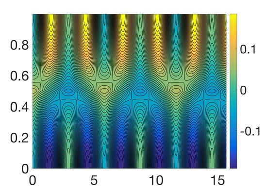
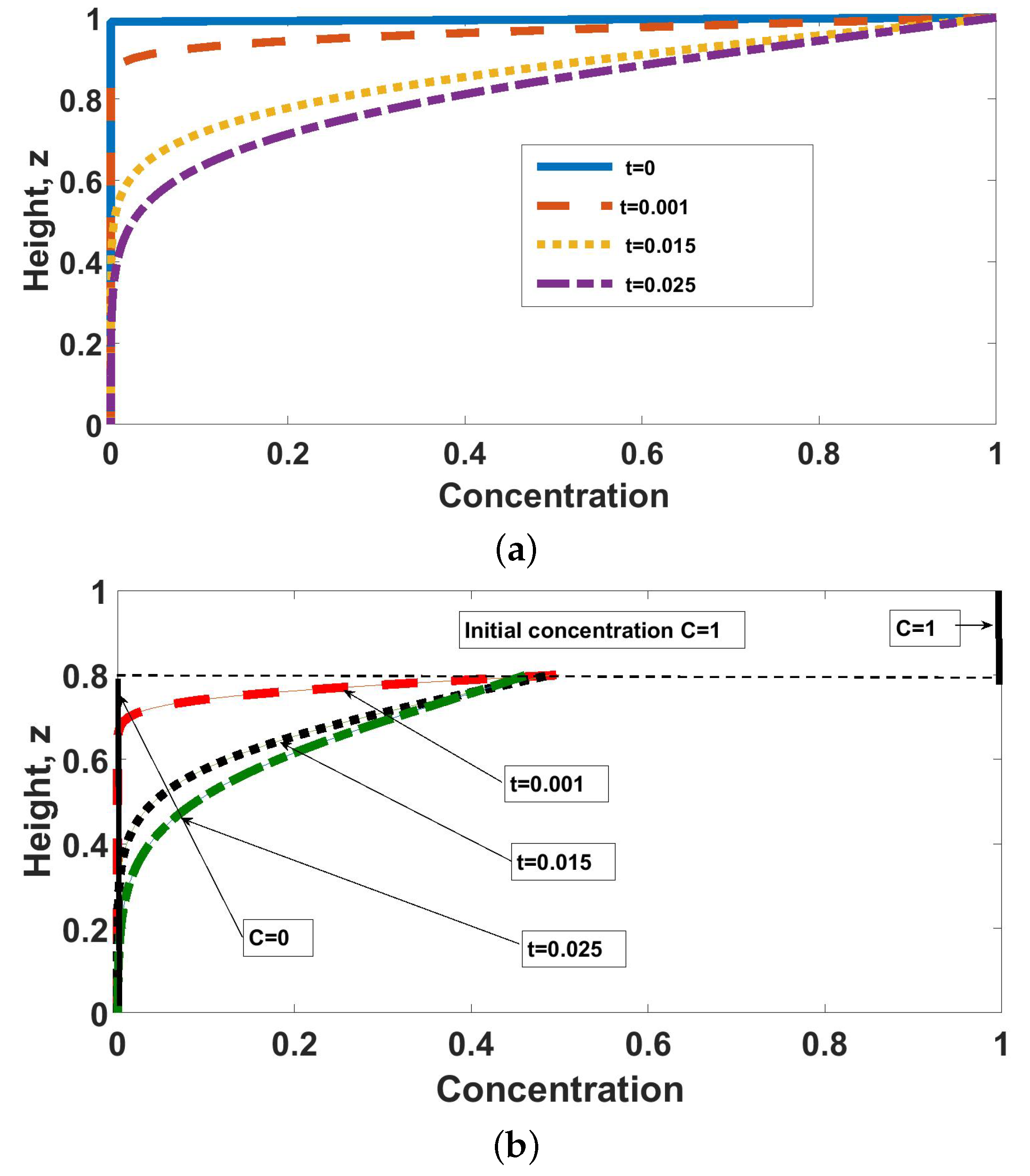
Its solution, which is derived in [12] with the positive z-direction pointing downward, is given by Equation (3), the plot of which appears on the left side of Figure 1:
The step-function base profile which satisfies the same diffusion equation and boundary conditions but with an assumed initial concentration given by
is described by Equation (5), the plot of which is depicted on the right side of Figure 1:
As depicted in Figure 1 and described in the schematic diagram (Figure 2), in the time-evolving base state model, the boundary layer thickens and gains potential energy over time until instability occurs at some critical time. The stability of such a base state requires the analysis of a set of coupled PDEs having coefficients that depend on both time and space. This approach has been considered by Foster [13,14] in his work involving the thermal boundary layer instability. The linear analysis proceeds by expanding the variables in a series of eigenfunctions having time-dependent coefficients and determining the critical wavenumber, defined as the one associated with the most dangerous disturbance among some set of initial conditions. Ennis-King and Patterson [12] point out a couple of drawbacks to this approach, namely the lack of a mathematically precise definition of critical time and the dependence of the latter on the set of initial conditions considered. These are some of the usual mathematical difficulties that one encounters when dealing with the stability of time-dependent states [15]. The alternative view considered by WH and VH presupposes that an initial boundary layer of some thickness and average concentration has developed and that its stability is then investigated to infinitesimal arbitrary time-dependent perturbations. This developed carbon-rich layer is heavier than the underlying brine, and is prone to buoyancy-induced Rayleigh–Taylor instability wherein diffusion has a stabilizing effect. Convection will set in once the layer attains a certain critical thickness and, by the same token, it has gained just enough potential energy that diffusion is no longer able to stabilize it [16]. From an experimental viewpoint, the two approaches are homologous in the sense that the step-function profile approach follows the same scenario as the time-evolving base state, with the exception that we stop the clock after some time has elapsed and ask whether the boundary layer that has formed thus far is stable to arbitrary and time-dependent disturbances. The only approximation made is that the carbon-rich layer is assumed to have some constant average concentration. This approximation leads to instability threshold conditions that are only conservative. However, this assumption can be relaxed and the approximation pushed a step further by including the variations of the concentration with depth within the carbon-rich boundary layer. Thus, with the approach adopted by VH and WH, the instability is characterized by a critical onset thickness instead of critical onset time. The former is mathematically more appealing and is amenable to analysis by simple analytical methods. Table 1 contrasts the predictions resulting from the transient and the step-function base states.
3. Mathematical Model
The mathematical model consists of the conservation equations of mass, momentum, and species within the Boussinesq approximation, which incorporate horizontal-to-vertical diffusion anisotropy, height-dependent permeability change, and a first-order reaction between the mixture and the host mineralogy [7,8,17]:
where p is the pressure and , g is the gravitational constant, is a unit vector in the positive z-direction, is a reference density, and w is the vertical component of the velocity vector field. The main dimensionless numbers that emerge are the Rayleigh–Darcy number , the height-dependent permeability function , the Damköhler number which represents the ratio of the reaction rate to the convective mass transfer rate, and depicts the diffusion anisotropy. The other symbols are defined as follows: is the coefficient of solutal expansion, d is the separation between the two horizontal boundaries, K is the permeability coefficient, is a reference CO2 concentration level, is the porosity, is the vertical component of the diffusion tensor, is the reaction rate, and the parameter numerically quantifies the value of the permeability variation. As detailed in either VH or WH, the model is simplified by considering the poloidal component of the divergence free velocity vector field, , and upon removing the pressure term, we obtain [7,8]:
where is the Dirac delta function, represents the horizontal gradient vector, and the prime symbol denotes differentiation with respect to z. The corresponding boundary conditions are:
Note that the exponential form of not only brings a tremendous simplification to the mathematical analysis, but its exponential dependence on depth is experimentally supported by the work of Klinkenberg [18] (i.e., the permeability shows a slight decrease with depth).
4. Stability Analysis
As detailed in VH and WH, due to the presence of the delta function term , the equations are solved in the two regions, where the boundary conditions at are used and where the boundary conditions at are used. The rest of the integration constants are obtained by imposing the continuity conditions for the velocity and all its derivatives at the interface . We impose the continuity of the concentration at the interface and a jump in the derivative of the concentration at . This comes out by integrating the concentration equation across the interface and leads to an expression for the Rayleigh–Darcy number as a function of both the wavenumber and the boundary layer thickness . Thus, with this approach the onset of the instability is accompanied by a jump in the concentration at the interface between the carbon-rich layer and the underlying ambient brine solution. The critical instability conditions can then be expressed as the minimum value of R attained at some critical value of the wavenumber for fixed , namely:
and the absolute minimum Rayleigh–Darcy number is then obtained by minimizing with respect to , namely:
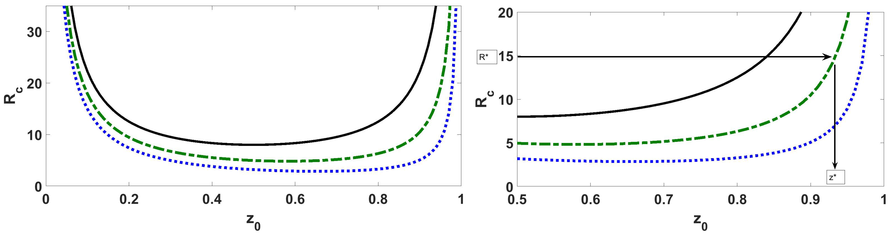
The derivation of a formula for , Equation (15), uses only analytical methods that are carried out using only paper and pencil. We refer the reader to VH and WH for the algebra details which are far too long to display here. This expression for reveals the explicit dependence of the critical threshold values on parameters. Thus, Equation (14) provides both the critical wavenumber and the critical depth of the carbon-rich boundary layer at the onset of convection. Figure 3 depicts the stability diagram showing a plot of R as function of for a selected set of values of the Damköher number . We note the emergence of a zero wavenumber instability in the limit of vanishing . This limit is used to carry out a long wavelength asymptotic analysis. Figure 3 also depicts the variation of with . We note that tends to infinity when either approaches 0 or 1 as both of these two limiting cases pertain to a layer that is stably stratified over the full vertical extent of the formation. One way to interpret this plot is as follows: consider a sequestration site whose physical constants and other externally imposed variables are such that R has a value and is described by the top continuous curve in Figure 3. By following the arrows from to the corresponding curve and then down, we retrieve the thickness of the boundary layer at the onset of convection, namely . If happens to be below the value of corresponding to that curve, then convection will be absent in that site and the dissolution of CO2 occurs solely by diffusion. The weakly nonlinear effects as well as the effect of permeability variations are shown in Figure 4. We note that an increase in permeability contrast, represented by the parameter ℓ, leads to instability onset occurring at thinner boundary layer depths. This is because an increase in permeability forces the intense convection flow to be confined at the top of the formation.
5. Two-Dimensional Results
We considered an alternative view of the convective stability associated with the geological sequestration of carbon dioxide, the solution of which is amenable to purely analytical methods using only paper and pencil. When the transient base state is considered, the carbon-rich boundary layer that forms at the top of the formation thickens and gains potential energy over time until instability occurs at some critical time. The determination of the stability threshold conditions requires the analysis of the stability of a base state that is both space- and time-dependent. One popular way to proceed is through defining the onset of convection in terms of critical time, the determination of which requires the use of similarity variables, quasi-normal modes, and energy methods combined with refined numerical techniques [19]. For instance, Xu et al. [20] used a Galerkin method to solve the stability problem. Upon invoking the dimensional scaling, , where denotes the critical onset time, they were able to predict a dimensional critical time years for a saline aquifer, the physical parameters of which are listed in [12].
An alternative view of the stability problem was pursued where it is supposed that an initial layer of some thickness and some average concentration has formed, leading to a base state having a step-function profile. The stability of the latter can then be investigated as a time-independent problem using a normal modes approach, leading to the onset of convection in terms of a critical boundary layer thickness. For instance, if we consider the data corresponding to the Sleipner site in the North Sea [21], we have a Rayleigh number . Upon using the stability diagram corresponding to the uniform permeability case, Figure 3, we have a critical boundary layer thickness of ≈0.2. For a formation of thickness 20 m, this corresponds to a dimensional critical thickness of ≈4 m and a critical time of 253 years, with m2· s−1.
As shown in VH, this approach shed light on the formation of the finger regime (Figure 5), and the influence of permeability variation with depth on the convective flow (Figure 5). The analysis was also able to shed some light on the interface motion and deformation that accompanies the jump in solute flux. For instance, it is found that in a some parameter range in the linear regime, the motion of the interface position, , is described by the following ordinary differential equation (ODE):
where coefficients and are expressions that are displayed in [8], is the scaled wavenumber, and is the critical thickness of the boundary layer. For a small interface deflection, we have:
whose solution is . Thus, The interface position evolves almost linearly with time until it reaches the upper boundary, signaling the end of the convection mixing within the formation.
6. Three-Dimensional Results
The analysis can be extended to the weakly nonlinear regime using only paper and pencil, as shown in VH and WH. For instance, VH considered a physical situation that can be analyzed using long-wavelength asymptotics to derive a 2D nonlinear evolution PDE for the leading order perturbation for the concentration. In this paper, we consider its 3D extension which is found to be described by:
where the parameter , which incorporates the various physical parameters that govern the problem, has a strong dependence on the permeability and for consistency with the long-wavelength limit [7]. The weakly nonlinear 2D analysis led the authors to posit a set of conditions for the appearance of the finger morphology shown in Figure 5, namely the presence of impervious boundaries, nonlinear regime, and the existence of a jump in the flux at the interface separating the carbon-rich layer from the underlying ambient brine. Based on the solution of the 2D evolution equation, it is further suggested that the finger pattern morphology results from a self-organization mechanism for the convective exchange of carbon at the interface to optimally adapt to the higher Rayleigh–Darcy number regime. In this paper, we highlight how to extend the 2D analysis to the 3D case by deriving an asymptotic solution to Equation (18) in order to examine the interfacial exchange between the carbon-rich and brine layers that leads to the three-dimensional finger pattern formation. Note that there is another way to proceed by performing a pattern formation analysis following the same line of analysis as in [22].
Upon considering the principal part of Equation (18), the solutions of which can be expressed as
where and are the two-dimensional wave-vectors and position vector, respectively, we find that the growth rate is given by
Thus, the static solution, , becomes unstable whenever . For simplicity and without loss of generality, we set . The weakly nonlinear development of this instability is investigated by deriving an asymptotic representation for the steady-state solution . We introduce the perturbation parameters, , and consider the following expansions near the instability threshold:
At the leading order in , we have
In view of the asymmetry that exists between the top and bottom fluid layers, we consider the hexagonal planform solution of Equation (23), namely:
At the order , we have
After expanding the right-hand side of Equation (25) and collecting similar terms, we conclude that the secular terms can be removed provided we set . The order of is then governed by the following problem:
whose solution is given by
Thus, up to , . Following the work of VH and WH, the order concentration quantities are then given by:
where and are the concentration in the brine () and in the carbon-rich layer (), respectively, and
7. Conclusions
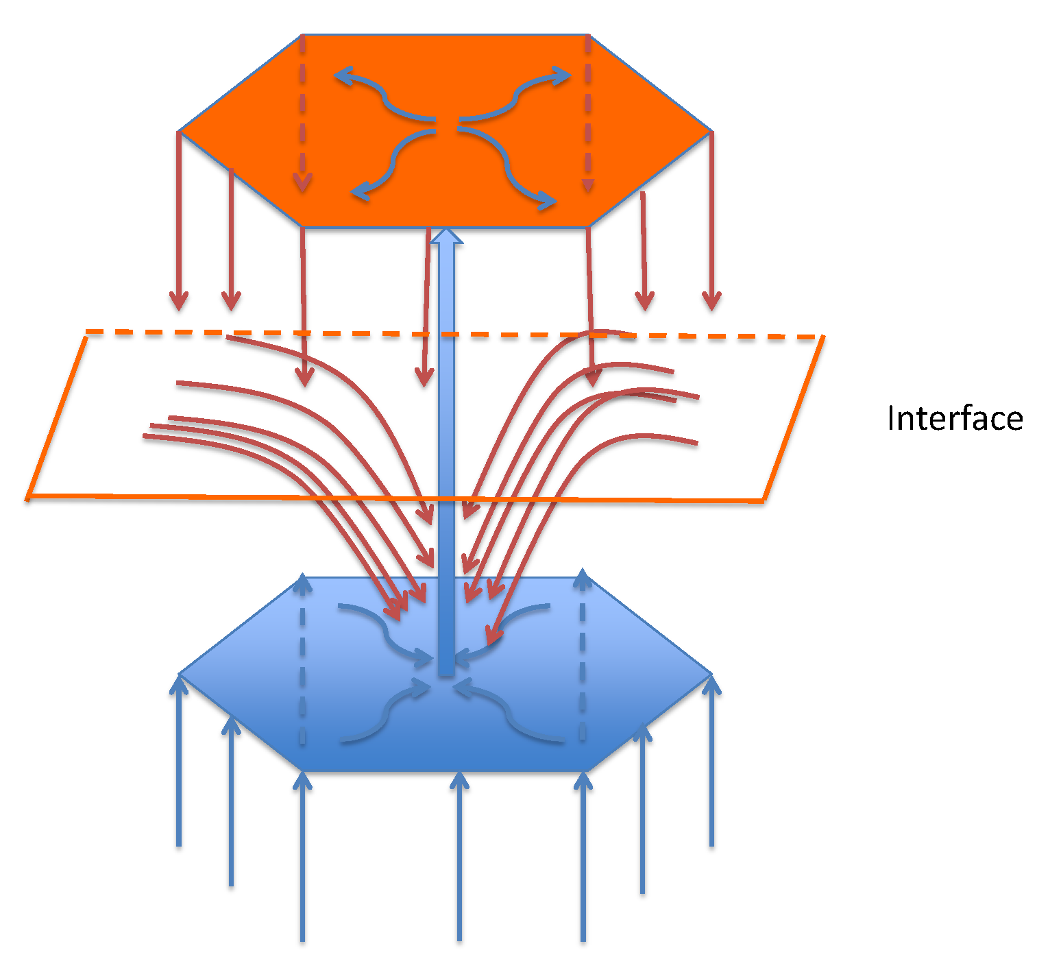
In this paper, we summarized some of the results obtained by VH and WH in their study of the instability associated with the sequestration of CO2 in geological formations. In the papers by VH and WH, an attempt was made to solve the stability problem by considering a different approach that is suitable to a time-independent analysis. The methods of normal modes and long wavelength asymptotics were used to perform both linear and nonlinear analyses, derive carbon fluxes at the interface between the carbon-rich layer and the ambient brine, use them to put forth the time evolution of the interface, and estimate an upper bound for the shutdown regime. In this paper, we also examined the extension to the three-dimensional case by first deriving the evolution equation for the planforn function, , and then solving it near onset. Its solution which is then used to plot the concentration profiles, shown in Figure 6, gives insight on how the exchange of carbon takes place at the interface. We invoked the asymmetry that exists between the top and bottom layers to assume a solution of the hexagonal form. Based on the findings in VH and WH and the three-dimensional extension carried out here, we also posited a possible scenario of how the ascending light currents and heavy descending currents may self-organize at the interface, as shown in Figure 7. Below the interface at , the light brine currents move up the walls of the lower hexagonal cell and converge toward the center of the upper hexagonal cell (), while above the interface, the heavy brine currents move also down the walls of the upper hexagonal cell and converge toward the center of lower cell. These conclusions are only qualitative. A quantitative evaluation of the results obtained so far through either the time-dependent or step-function profiles is difficult due to the lack of realistic data, which can be obtained only through large-scale experiments at reservoir conditions [21].
Funding
This research received no external funding.
Conflicts of Interest
The author declares no conflict of interest.
References
- Sedjo, R.; Sohngen, B. Carbon sequestration in forests and soils. Annu. Rev. 2012, 4, 127–144. [Google Scholar] [CrossRef]
- Bachu, S. Sequestration of CO2 in geological media in response to climate change: road map for site selection using the transform of the geological space into the CO2 phase space. Energy Convers. Manag. 2002, 43, 87–102. [Google Scholar] [CrossRef]
- Bachu, S. Sequestration of CO2 in geological media: Criteria and approach for site selection in response to climate change. Energy Convers. Manag. 2000, 41, 953–970. [Google Scholar] [CrossRef]
- U.S. Department of Energy. Carbon Sequestration Key R&D Programs and Initiatives. Available online: https://www.energy.gov/fe/science-innovation/carbon-capture-and-storage-research (accessed on 23 August 2018).
- International Panel on Climate Change. Carbon Dioxide Capture and Storage; Cambridge University Press: Cambridge, UK, 2005. [Google Scholar]
- Huppert, H.E.; Neufeld, J.A. The fluid mechanics of carbon dioxide sequestration. Annu. Rev. Fluid Mech. 2014, 46, 255–272. [Google Scholar] [CrossRef]
- Vo, L.; Hadji, L. Weakly nonlinear convection induced by the sequestration of CO2 in a perfectly impervious geological formation. Phys. Fluids 2017, 29, 127101. [Google Scholar] [CrossRef]
- Wanstall, C.T.; Hadji, L. A step function density profile model for the convective stability of CO2 geological sequestration. J. Eng. Math. 2018, 108, 53–71. [Google Scholar] [CrossRef]
- De Paoli, M.; Zonta, F.; Soldati, A. Influence of anisotropic permeability on convection in porous media: Implications for geological CO2 sequestration. Phys. Fluids 2016, 28, 056601. [Google Scholar] [CrossRef]
- Meybodi, H.M.; Hassanzadeh, H. Stability analysis of two-phase buoyancy-driven flow in the presence of a capillary transition zone. Phys. Rev. E 2013, 87, 033009. [Google Scholar] [CrossRef]
- Meybodi, H.M. Stability analysis of dissolution-driven convection in porous media. Phys. Fluids 2017, 29, 014102. [Google Scholar] [CrossRef]
- Ennis-King, J.P.; Paterson, L. Role of convective mixing in the long-term storage of carbon dioxide in deep saline formulations. Soc. Pet. Eng. 2005, 10, 349–356. [Google Scholar]
- Foster, T. Onset of convection in a layer of fluid cooled from above. Phys. Fluids 1965, 8, 1770–1774. [Google Scholar] [CrossRef]
- Foster, T. Onset of manifest convection in a layer of fluid with time-dependent surface temperature. Phys. Fluids 1969, 12, 2482–2487. [Google Scholar] [CrossRef]
- Drazin, P.G.; Reid, W.H. Hydrodynamic Stability; Cambridge University Press: Cambridge, UK, 2004. [Google Scholar]
- Batchelor, G.; Nitsche, J. Instability of stationary unbounded stratified fluid. J. Fluid Mech. 1991, 227, 357–391. [Google Scholar] [CrossRef]
- Hill, A.; Morad, M. Convective stability of carbon sequestration in anisotropic porous media. Proc. R. Soc. A 2014, 470, 2170. [Google Scholar] [CrossRef]
- Klinkenberg, K. The permeability of porous media to liquids and gases. In Drilling and Production Practice, American Petroleum Institute; American Petroleum Institute: Washington, DC, USA, 1941. [Google Scholar]
- Riaz, A.; Hesse, M.; Tchelepi, H.A.; Orr, F.M. Onset of convection in a gravitationally unstable diffusive boundary layer in porous media. J. Fluid Mech. 2006, 548, 87–111. [Google Scholar] [CrossRef]
- Xu, X.; Chen, S.; Zhang, D. Convective stability analysis of the long-term storage of carbon dioxide in deep saline aquifers. Adv. Water Resour. 2006, 29, 397–407. [Google Scholar] [CrossRef]
- Neufeld, J.; Hesse, M.; Riaz, A.; Hallworth, M.; Techelepi, H.; Huppert, H. Convective dissolution of carbon dioxide in saline aquifers. Geophys. Res. Lett. 2010, 37, L22404. [Google Scholar] [CrossRef]
- Riahi, N. Nonlinear convection in a porous layer with finite conducting boundaries. J. Fluid Mech. 1983, 129, 153–171. [Google Scholar] [CrossRef]
Figure 1.
The two plots contrast the time-evolving base state profile, Equation (3) (a) and the step-function base profile, Equation (5) (b). In the former, a carbon-rich layer forms at the top and grows with time until instability onset, while in the latter it is assumed that after an initial layer of thickness and of average concentration has initially formed, its stability to arbitrary infinitesimal time-dependent perturbations is investigated.

Figure 2.
A schematic diagram contrasting the two base configurations.
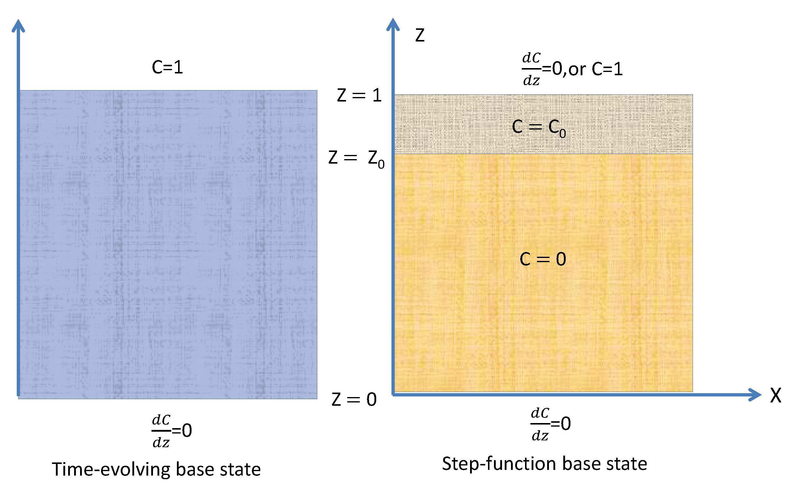
Figure 3.
Suppose that for some sequestration site, the physical parameters and the concentration level are such that the Rayleigh–Darcy number is . Then, the thickness of the boundary layer at which the instability sets in is given by . If happens to be less than the absolute minimum for that particular site, then convection will be absent and the carbon dioxide will dissolve by diffusion alone. Note also that the magnitude of the critical Rayleigh number can be large, so the large R values encountered in sequestration sites is not necessarily an indication of a turbulent mixing [7]. Reproduced with permission from [7].
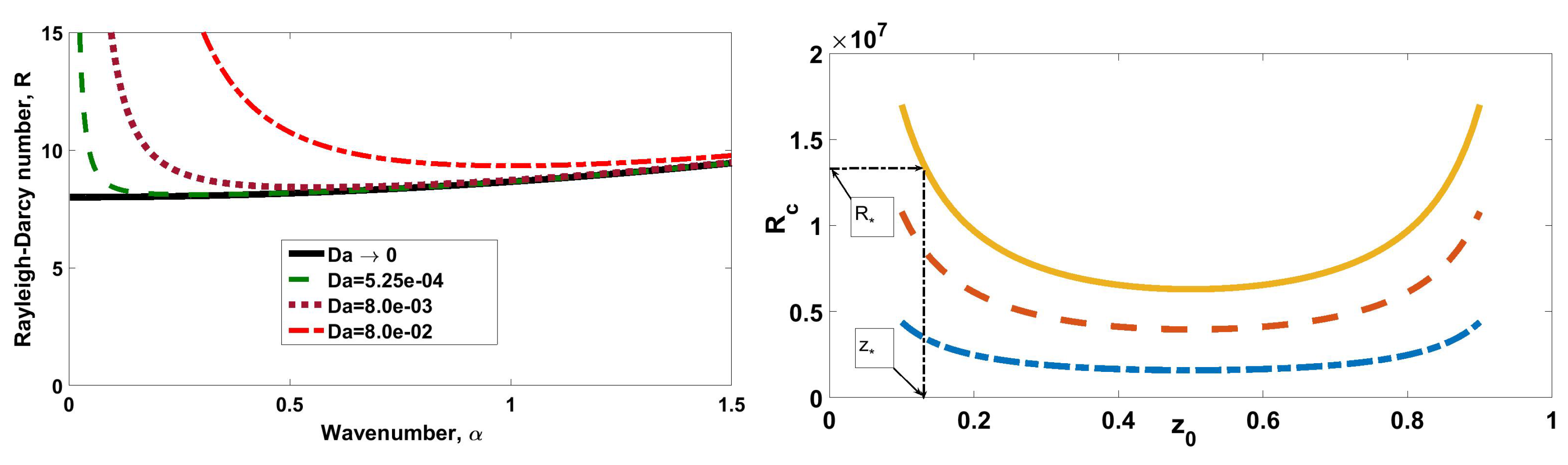
Figure 4.
The critical Rayleigh number obtained through the weakly nonlinear analysis is plotted as a function of for three distinct values of ℓ, namely (continuous line), (dashed line), and (dotted line) [8]. Note that values get very large as gets closer to 1. Furthermore, only the interval is plotted since convection set in first at the top half of the formation. Reproduced with permission from [8].

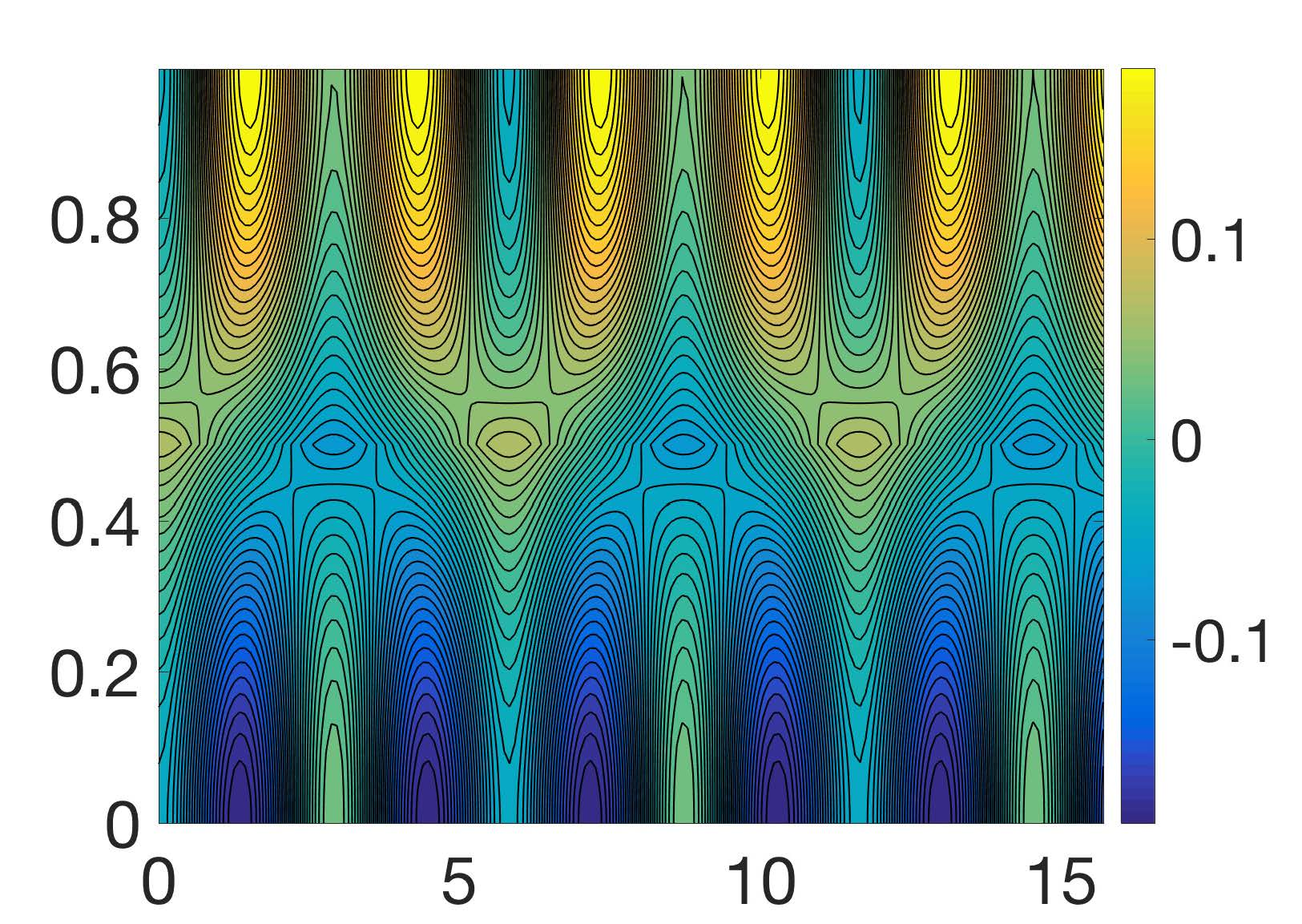
Figure 5.
Plot of the concentration as function of the deviation from onset of convection, namely where denotes the amplitude of motion and are the contributions to the concentration. A large deviation leads to the appearance of finger morphology (a) [7]. Plot of the streamlines for parameter values, , and (b) [8]. As the permeability contrast between the top and bottom regions increases, high intensity convection gets confined at the top and penetrates the bottom regions, thus inducing only a low-intensity convective flow there. Reproduced with permission from [7,8].
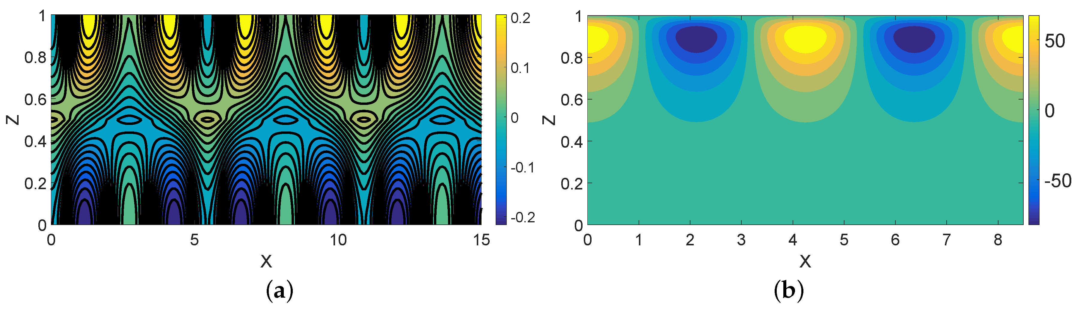
Figure 6.
Plot of the concentration as a function of the deviation from onset of convection, namely , where denotes the amplitude of motion and are the contributions to the concentration. In this case, and is given by Equation (29). The plots depict as slices by planes , , and . We note that the slice reduces to the two-dimensional case studies in VH as shown in Figure 5. The z-slice covers a wider region in the -plane. The parameters used are as follows: , , , , , and .
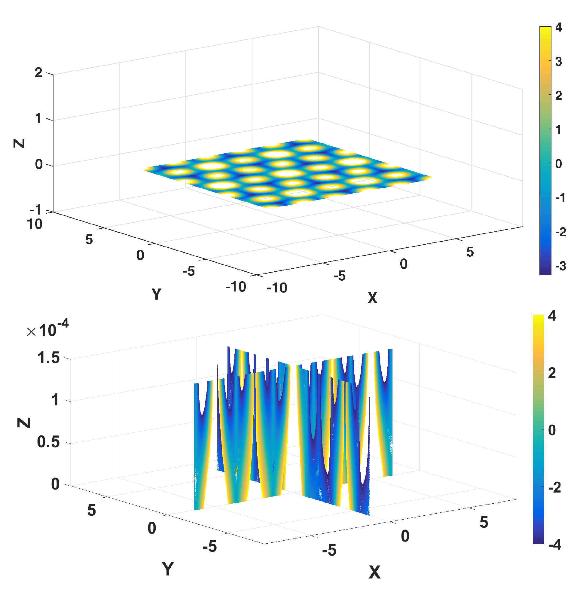
Figure 7.
Schematic diagram depicting a possible scenario of the ascending light currents and descending carbon-rich currents near the interface at .
Figure 7.
Schematic diagram depicting a possible scenario of the ascending light currents and descending carbon-rich currents near the interface at .


Table 1.
Table contrasting the stability characteristics of the two base states.
| Time-Evolving Base State | Step-Function Base Profile |
|---|---|
| Onset as function of time | Onset as function of boundary layer thickness |
| Lack of a precise definition of stability | Mathematically precise definition of stability |
| Stability of a time-dependent state | Steady analysis via normal modes |
| Requires refined numerical techniques | Paper-and-pencil analysis |
| Numerical tracking of the interface fluxes | Closed-form expressions for the interface fluxes |
| Numerical extension to nonlinear regime | Analytically tractable weakly nonlinear convection state |
| Challenging extension to three-dimensional case | Analytically tractable pattern formation study |
| Approximate instability threshold values | Conservative instability threshold values |
© 2018 by the author. Licensee MDPI, Basel, Switzerland. This article is an open access article distributed under the terms and conditions of the Creative Commons Attribution (CC BY) license (http://creativecommons.org/licenses/by/4.0/).
Share and Cite
MDPI and ACS Style
Hadji, L. A Simple Analytical Model for Estimating the Dissolution-Driven Instability in a Porous Medium. Fluids 2018, 3, 60. https://doi.org/10.3390/fluids3030060
AMA Style
Hadji L. A Simple Analytical Model for Estimating the Dissolution-Driven Instability in a Porous Medium. Fluids. 2018; 3(3):60. https://doi.org/10.3390/fluids3030060
Chicago/Turabian StyleHadji, Layachi. 2018. "A Simple Analytical Model for Estimating the Dissolution-Driven Instability in a Porous Medium" Fluids 3, no. 3: 60. https://doi.org/10.3390/fluids3030060