Flow and Nematic Director Profiles in a Microfluidic Channel: The Interplay of Nematic Material Constants and Backflow

Abstract

We numerically and analytically study the flow and nematic order parameter profiles in a microfluidic channel, within the Beris–Edwards theory for nematodynamics, with two different types of boundary conditions—strong anchoring/Dirichlet conditions and mixed boundary conditions for the nematic order parameter. We primarily study the effects of the pressure gradient, the effects of the material constants and viscosities modelled by a parameter $L_2$ and the nematic elastic constant $L^{\ast }$, along with the effects of the choice of the boundary condition. We study continuous and discontinuous solution profiles for the nematic director and these discontinuous solutions have a domain wall structure, with a layered structure that offers new possibilities. Our main results concern the onset of flow reversal as a function of $L^{\ast }$ and $L_2$, including the identification of certain parameter regimes with zero net flow rate. These results are of value in tuning microfluidic geometries, boundary conditions and choosing liquid crystalline materials for desired flow properties.

1. Introduction

Nematic liquid crystals are classical examples of partially ordered complex liquids for which the constituent molecules have translational freedom but exhibit a degree of long-range orientational ordering or certain preferred directions of averaged molecular alignment, that vary in space and time [1]. The nematic hydrodynamics is particularly rich because of the intrinsic coupling between fluid motion and nematic molecular orientations i.e., the fluid motion influences the nematic orientational ordering and equally, the inhomogeneities in the orientational ordering have a kick-back effect on the fluid flow, a phenomenon known as “backflow” [2]. Backflow has no counterpart in conventional isotropic Newtonian fluids. Consequently, nematics can offer unusual mechanical and rheological properties compared to their Newtonian counterparts, such as complex wetting transitions, surface effects and stable topological defects. Backflow is of fundamental scientific interest and equally, has practical consequences on switching rates of liquid crystal display devices and their refresh times [3,4].

There are two popular hydrodynamic theories for nematic liquid crystals in the literature—the Ericksen–Leslie theory [5,6] and the Beris–Edwards model [7]. In the Ericksen–Leslie framework, we have two variables—the flow field and the nematic director, which is interpreted as the direction of preferred averaged molecular alignment in space. The typical mathematical framework comprises the incompressibility constraint and evolution equations for the flow field and the nematic director. The evolution equations for the flow field and the nematic director are intrinsically coupled with new anisotropic stresses, compared to the isotropic Newtonian counterpart, and the solution landscapes depend on flow parameters (such as the pressure gradient) and nematic parameters (nematic material constants, temperature, boundary conditions for the nematic director and nematic viscosities) [8]. The Ericksen–Leslie theory for nematodynamics is based on the premise that the nematic is purely uniaxial, with one single distinguished direction of orientational ordering, referred to as “director”, with a constant degree of orientational order. As said before, the director is interpreted as the single preferred direction of molecular alignment in the sense that all directions perpendicular to the director are physically equivalent. Hence, the Ericksen–Leslie theory is hugely successful for modelling situations that are expected to have a uniform degree of nematic ordering; this usually holds for defect-free situations or for certain choices of material constants that promote perfect nematic ordering such as the vanishing elastic constant limit of the Landau-de Gennes theory studied in [9]. However, the Ericksen–Leslie theory cannot capture sharp variations in the degree of nematic ordering, complicated topological defects and biaxiality, for which there is a primary and secondary direction of preferred molecular alignment, since the Ericksen–Leslie theory only has two dependent variables. The Beris–Edwards theory is more general than the Ericksen–Leslie since it employs the Landau-de Gennes $\mathit{Q}$-tensor order parameter to describe the nematic orientational ordering. The Landau-de Gennes $\mathit{Q}$-tensor order parameter is a symmetric, traceless $3\times 3$ matrix that contains information about the preferred directions of nematic molecular alignment and the degree of ordering about these directions within its eigenvectors and eigenvalues respectively [9,10,11]. The Landau-de Gennes $\mathit{Q}$-tensor can capture both uniaxial and biaxial states, along with variable orientational order and is hence better suited to capture finer structural details and topological defects. The evolution equations for the flow field and the $\mathit{Q}$-tensor are again coupled through “coupling stresses”. A detailed discussion of the Beris–Edwards model and its connections to closely related models can be found in the literature [12,13,14].

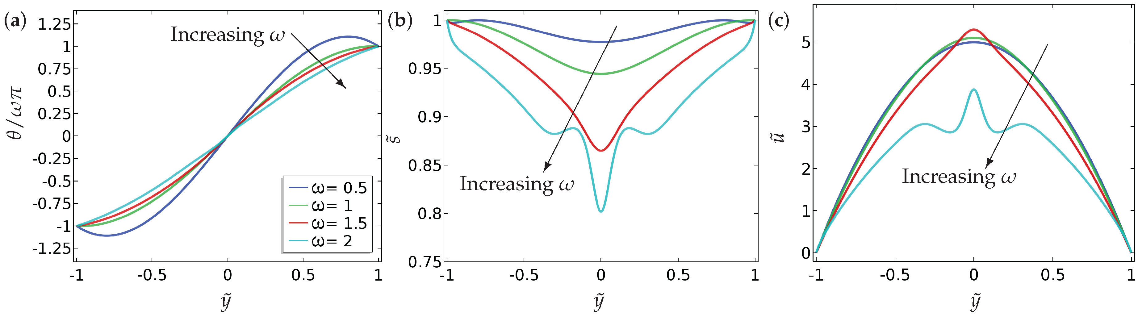
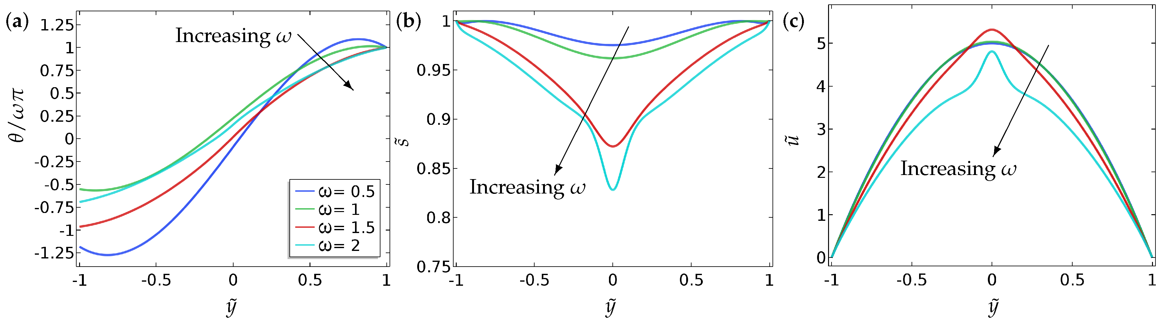
We work in a reduced Beris–Edwards framework to model a microfluidic channel, with an applied pressure gradient to induce fluid flow, and different types of boundary conditions for a reduced $\mathit{Q}$-tensor on the channel walls with the usual no-slip boundary conditions for the flow field. We use a reduced $\mathit{Q}$-tensor, which only has two degrees of freedom, in contrast to the usual five degrees of freedom in a three-dimensional approach. This reduced approach has been successfully used for severely confined systems elsewhere [15,16] and can be related to the usual Landau-de Gennes $\mathit{Q}$-tensor explicitly [17]. In particular, we model the microfluidic channel as a two-dimensional domain and this reduced approach is successful in capturing the in-plane system characteristics. The two degrees of freedom of the reduced $\mathit{Q}$-tensor are an angle $\theta$ that describes the preferred in-plane alignment of the nematic molecules or the direction of the nematic director $\mathit{n}$ in the plane, and a scalar order parameter s, that is a measure of the degree of orientational order about the director $\mathit{n}$. We note that the Ericksen–Leslie framework does not include the order parameter s. The Beris–Edwards system can be recast as a coupled system for s, $\theta$ and the flow field parameterised by u (since we assume unidirectional channel flow). We study the effects of certain key variables on the long-time or equilibrium profiles for s, $\theta$ and u. Namely, we look at the effects of the pressure gradient $p_x$, the nematic elastic constant, the nematic material constants and viscosities (modelled by $L_2$) and the anchoring conditions for $\theta$ (modelled by either the winding number $\omega$ or the surface anchoring coefficient B). For small $L_2$, the evolution equation for the flow field effectively reduces to the Navier–Stokes equation and we recover the usual Poiseuille flow. However, the flow field does influence the $\theta$ profiles in this regime and we carry out some explicit analysis to compute the s and $\theta$ profiles in this limit, for both small and large $L^{\ast }$. 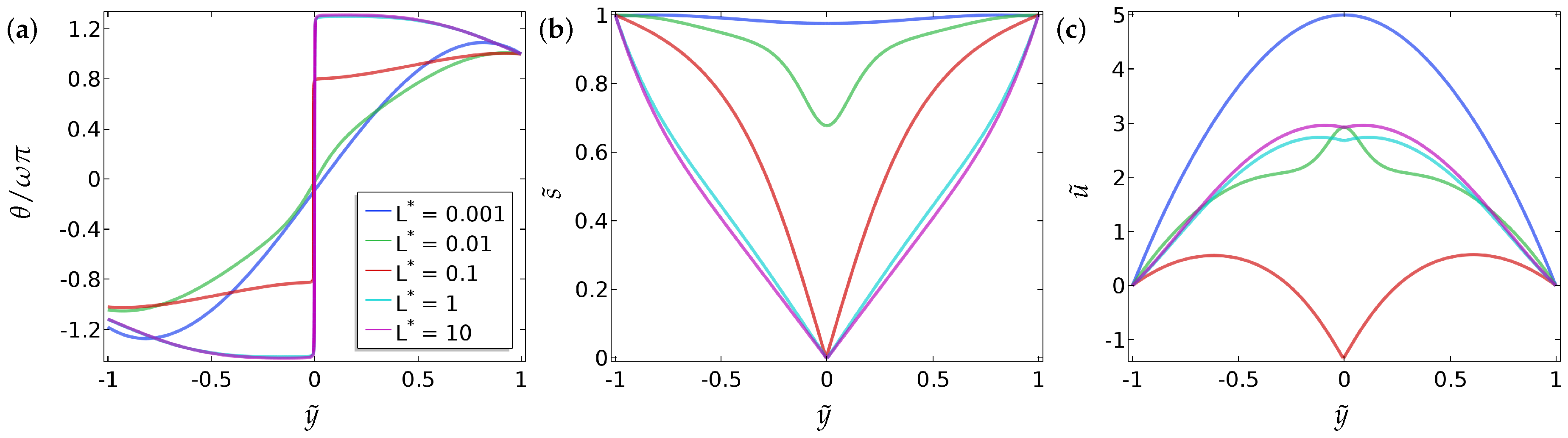The analysis captures both continuous and discontinuous solution profiles for $\theta$; the discontinuous profiles are featured by domain walls with layered structures such that $\theta$ jumps abruptly across an interface. Again, the discontinuous solutions cannot be captured by the Ericksen–Leslie approach. The discontinuous solutions are the analogue of the well studied “order-reconstruction” solutions [18], with the novel feature of flow effects. For small $p_x$, the flow is negligible as expected. The most interesting regime is when $p_x$ and $L_2$ are of comparable magnitude and there is two-way coupling between the flow and nematic order, where the effects of backflow are most pronounced. We expect the asymptotic analysis in this paper to be useful for subsequent detailed analysis of the Beris–Edwards system in this interesting regime.

There is a large body of existing literature on the Ericksen–Leslie theory and the Beris–Edwards theory. For example, an extensive review of existence and regularity results in the Ericksen–Leslie framework can be found in [19]. In [20], the authors use perturbation methods in the Ericksen–Leslie framework to study the effects of backflow on defect dynamics. In parallel, there are several papers that focus on the role of backflow in the hydrodynamics of defects, in the Beris–Edwards framework, see for example [12,21,22]. In recent years, there are rigorous existence and regularity results for the Beris–Edwards framework too [11,14,23] and numerical simulations for microfluidic set-ups in [24,25]. The various dynamical theories of nematic liquid crystals and the key results are surveyed in [26] and in [27]; the authors rigorously derive the Ericksen–Leslie equations from the Beris–Edwards model. In [28], the authors use a lattice-Boltzmann algorithm to study nematodynamics in a microfluidic channel, in the Beris–Edwards framework, with both Dirichlet and mixed boundary conditions on the channel walls. The emphasis is on the flow rate as a function of the applied pressure gradient and the qualitative effects of the boundary conditions on the director profiles. Our setting is similar but not the same as in [28]. For example, our Dirichlet conditions are inhomogeneous i.e., different fixed boundary conditions on the two bounding surfaces, whereas the authors employ the same Dirichlet condition on both surfaces in [28]. A large part of the elegant asymptotics in [28] is carried out in the $L^{\ast }\to 0$ limit, for which we expect a uniform degree of nematic order or $s\approx 1$ almost everywhere. This limit cannot capture the discontinuous solutions for $\theta$ described above. Importantly, our emphasis is on “flow reversal" as a function of the pressure gradient, the material and temperature-dependent parameter $L_2$ and the re-scaled elastic constant $L^{\ast }$ and this is not addressed in [28]. In fact, flow reversal or flow in the direction of increasing pressure gradient is a distinct manifestation of backflow, only observable for $L_2$ large enough; this warrants further study in the future.

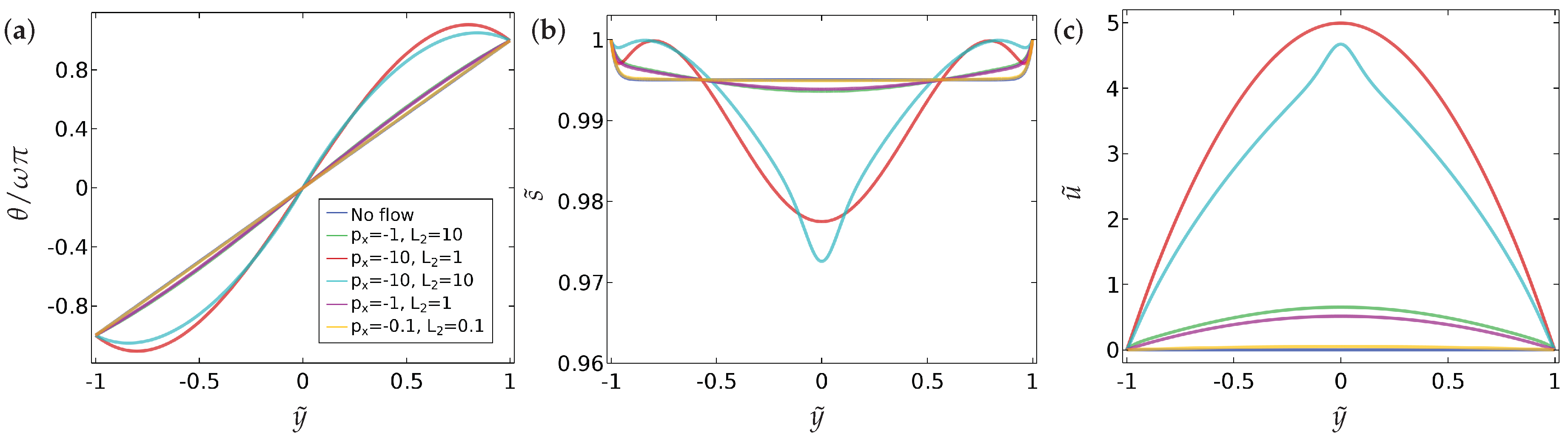
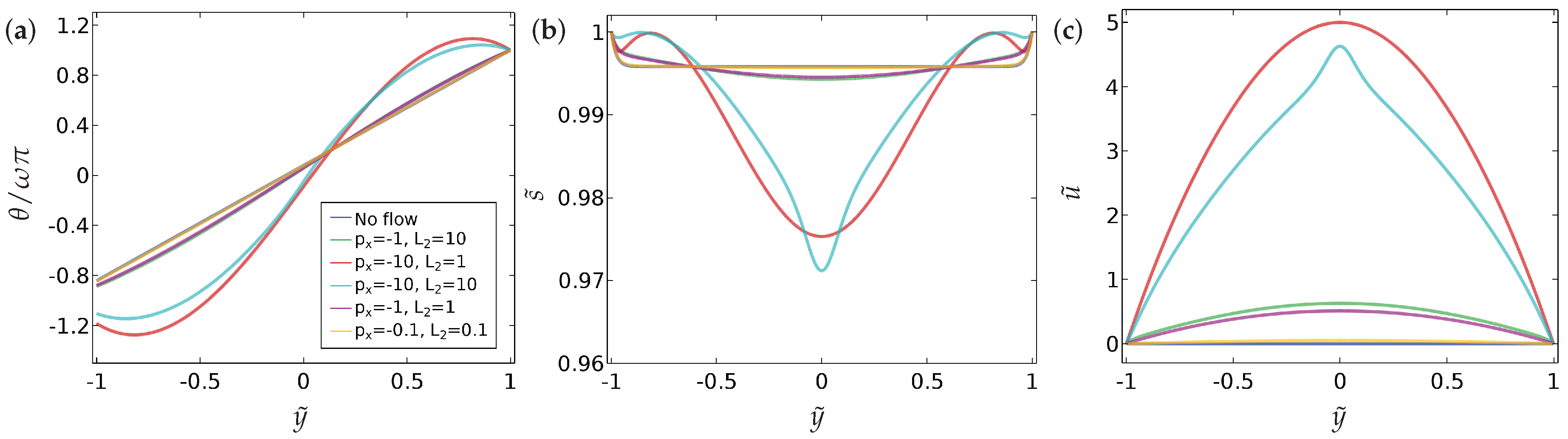
Our main findings can be summarised as follows.

(a)

We compute a phase plane in terms of $L^{\ast }$ and $L_2$, for a fixed $p_x$, which demarcates regions of fluid flow in the direction of decreasing pressure from regions of fluid flow in the direction of increasing pressure and this flow reversal is a clear manifestation of backflow.

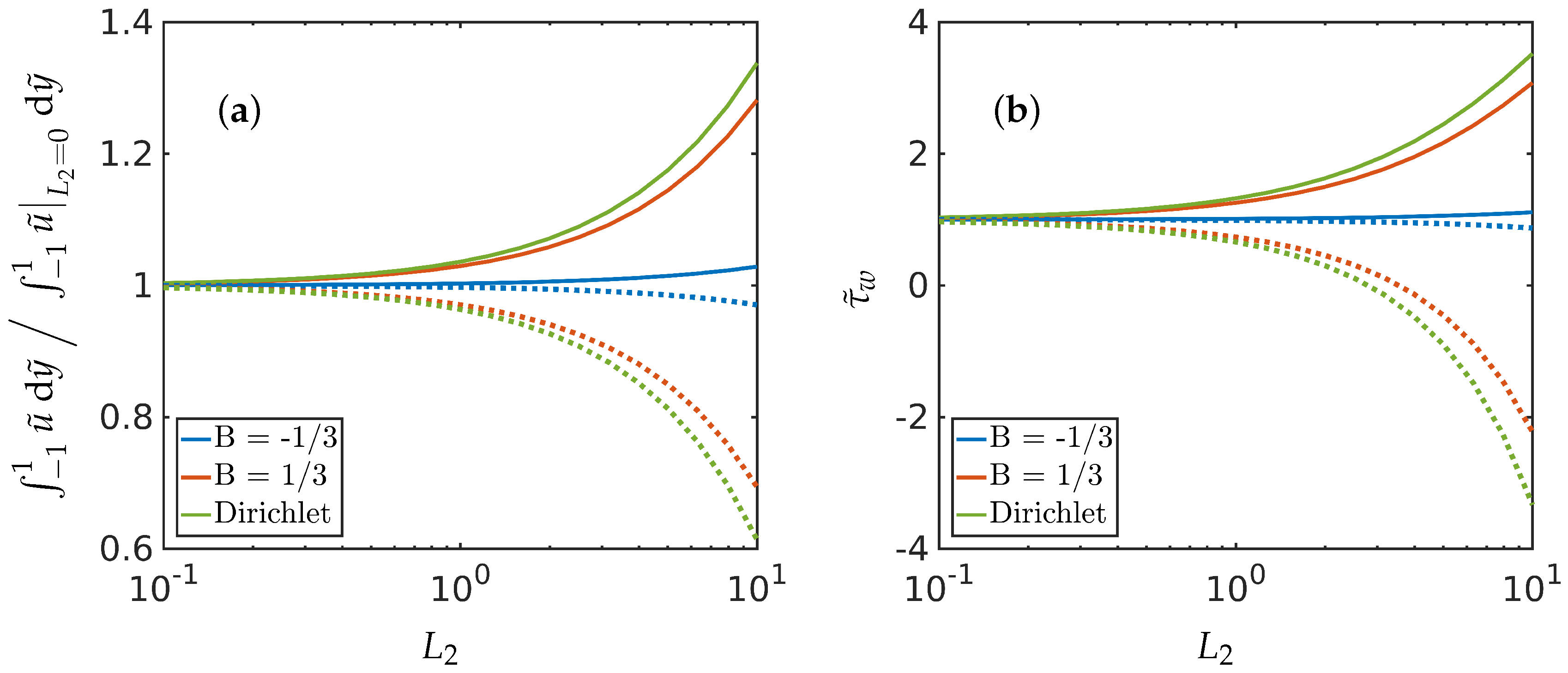
(b)

We compute the total flow rates in different parameter regimes. In particular, we show that backflow can be attained for a window of values of $L^{\ast }$ i.e., $L_{crit,1}^{\ast }<L^{\ast }<L_{crit,2}^{\ast }$ and these critical values depend on $p_x,L_2$, the boundary conditions and other material parameters.

(c)

We study two different kinds of boundary conditions for $\theta$—Dirichlet and mixed boundary conditions. The mixed boundary conditions are phrased in terms of an anchoring coefficient B on the bottom surface and accompanied by a Dirichlet condition on the top surface. The mixed boundary conditions offer greater scope for tuning the solution landscape.

(d)

We perform some investigations on how we can choose a suitable initial condition to attain the discontinuous solution for $\theta$ at long times, and this may be useful for studying multistability in such model settings.

The paper is organised as follows. In Section 2, we present the governing equations, the boundary conditions and the initial conditions. In Section 3, we present our results on the effects of $p_x,L_2$, $\omega$ and $L^{\ast }$. In Section 4, we perform the explicit analysis in the small $L_2$ limit and in Section 5, we give some conclusions.

2. Theory

We study spatio-temporal pattern formation in a long microfluidic channel

$$\begin{array}{c}\hfill \mathsf{\Omega }=\left\{(x,y)\in {\mathbb{R}}^2;-H<x<H;-L<y<L\right\}\end{array}$$

(1)

where $L/H\ll 1$, filled with nematic liquid crystals under the action of a pressure gradient applied at the end $x=-H$ in the x direction. This pressure gradient naturally induces a fluid flow and we assume a unidirectional channel flow in the x-direction. There are two main macroscopic variables of interest: the flow field $\mathit{u}=\left(u\left(x,y,t\right),0,0\right)$, where t is time, and the nematic order parameter, which is a measure of the nematic ordering. We work in a reduced two-dimensional Landau-de Gennes framework, similar to the setting in [15,16] for which the nematic order parameter $\mathit{q}$ is a symmetric, traceless $2\times 2$ matrix, with two degrees of freedom. Equivalently, we can write $\mathit{q}=s\left(\mathit{n}⨂\mathit{n}-\mathit{I}/2\right)$ where $\mathit{I}$ is the 2D identity matrix, with $s=\sqrt{2}\left|\mathit{q}\right|$ being the scalar order parameter and $\mathit{n}=(\cos \theta ,\sin \theta )$ being the two-dimensional director. The general Landau-de Gennes nematic order parameter, $\mathit{Q}$, is a symmetric, traceless $3\times 3$ matrix with five degrees of freedom but for severely confined systems, where the vertical z-dimension is much smaller than the lateral dimensions; it is reasonable to assume that structural details are independent of the z-coordinate and we can relate the reduced tensor, $\mathit{q}$ in this paper to the full Landau-de Gennes $\mathit{Q}$ tensor as has been done in [17]. A reduced approach, such as the one employed in this paper and others, is analytically and computationally more efficient and is a physically relevant approach for severely confined systems.

We work within the standard and powerful Beris–Edwards theoretical framework for nematodynamics [24]. There are three governing equations: the incompressibility constraint, an evolution equation for the flow field, which is essentially the Navier–Stokes equation with an additional stress ($\mathit{\sigma }$) due to the nematic ordering and an evolution equation for $\mathit{q}$, which has an additional stress induced by the fluid vorticity. The governing partial differential equations are given below.

$$\nabla ·\mathit{u}=0,\rho \frac{D\mathit{u}}{Dt}=-\nabla p+\nabla ·\left[\mu \left(\nabla \mathit{u}+{(\nabla \mathit{u})}^{\prime }\right)+\mathit{\sigma }\right],$$

(2)

where $\frac{D}{Dt}=\frac{\partial }{\partial t}+\mathit{u}·\nabla$ is the material derivative, $\rho$ and $\mu$ are the density and viscosity of the fluid medium, p is the hydrodynamic pressure, $\mathit{u}$ is the fluid velocity, and prime ${}^{\prime }$ denotes the transpose. The nematic stress ($\mathit{\sigma }$) is [9,24,29]

$$\mathit{\sigma }=\mathit{qh}-\mathit{hq},\mathrm{and}\mathit{h}=\kappa {\nabla }^2\mathit{q}+a\mathit{q}-c\mid \mathit{q}{\mid }^2\mathit{q},$$

(3)

where $s=\sqrt{2}\left|\mathit{q}\right|$ is the scalar order parameter, $\mathit{h}$ is the molecular field, $\kappa$ is the nematic elastic constant and a and c are parameters related to the temperature and material properties. We work with temperatures below the nematic–isotropic transition temperature and hence we take $a>0$. The evolution equation for the $\mathit{q}$ tensor is given by [11,29]

$$\frac{D\mathit{q}}{Dt}=\mathit{q}\mathit{\xi }-\mathit{\xi }\mathit{q}+\frac{1}{\gamma }\mathit{h},$$

(4)

where $\gamma$ is the rotational diffusion constant [10,21] and $\mathit{\xi }$ is the anti-symmetric part of the velocity gradient tensor. We can also identify $\mathit{q}$ with a two-dimensional vector: $\mathit{q}=(q_{11},q_{22})$ where $q_{11}=\frac{s}{2}\cos 2\theta ;$ $q_{12}=\frac{s}{2}\sin 2\theta .$

We assume that all quantities of interest only depend on y i.e., we work in a reduced one-dimensional setting, which is a physically relevant setting for very long channels with small height. Equations (2) and (4) can be recast in terms of the order parameter (s) and the director angle ($\theta$) in one spatial dimension as

$$\begin{array}{cc}\hfill \frac{\partial s}{\partial t}-\frac{\kappa }{\gamma }{s}_{yy}& =-\frac{4\kappa s}{\gamma }{\theta }_y^2-\frac{s}{\gamma }\left(\frac{c}{2}{s}^2-a\right),\hfill \end{array}$$

(5)

$$\begin{array}{cc}\hfill \frac{\partial \theta }{\partial t}-\frac{\kappa }{\gamma }{\theta }_{yy}& =-u_y+\frac{2\kappa }{s\gamma }\left(s_y{\theta }_y\right),\hfill \end{array}$$

(6)

$$\begin{array}{cc}\hfill \rho \frac{\partial u}{\partial t}-\mu u_{yy}& =-p_x+\kappa {\left(s^2{\theta }_y\right)}_{yy}.\hfill \end{array}$$

(7)

Using the following scalings,

$$\begin{array}{c}\hfill y=L\tilde{y},t=\frac{\gamma L^2}{\kappa }\tilde{t},s=\tilde{s}\sqrt{\frac{2a}{c}},u=\frac{\kappa }{\gamma L}\tilde{u},p_x=\frac{\mu \kappa }{\gamma L^3}{\tilde{p}}_x,\end{array}$$

(8)

Equations (5)–(7) can be non-dimensionalised as

$$\begin{array}{cc}\hfill {\tilde{s}}_{\tilde{t}}-{\tilde{s}}_{\tilde{y}\tilde{y}}& =-4\tilde{s}{\theta }_{\tilde{y}}^2-\frac{\tilde{s}}{L^{\ast }}\left({\tilde{s}}^2-1\right),\hfill \end{array}$$

(9)

$$\begin{array}{cc}\hfill {\theta }_{\tilde{t}}-{\theta }_{\tilde{y}\tilde{y}}& =-{\tilde{u}}_{\tilde{y}}+\frac{2}{\tilde{s}}{\tilde{s}}_{\tilde{y}}{\theta }_{\tilde{y}},\hfill \end{array}$$

(10)

$$\begin{array}{cc}\hfill L_1{\tilde{u}}_{\tilde{t}}-{\tilde{u}}_{\tilde{y}\tilde{y}}& =-{\tilde{p}}_x+L_2{\left({\tilde{s}}^2{\theta }_{\tilde{y}}\right)}_{\tilde{y}\tilde{y}},\hfill \end{array}$$

(11)

where

$$\begin{array}{cccccc}\hfill L^{\ast }& =\frac{\kappa }{a{L}^2},\hfill & \hfill L_1& =\frac{\rho \kappa }{\mu \gamma },\hfill & \hfill L_2& =\frac{2a\gamma }{c\mu },\hfill \end{array}$$

(12)

and L is the half-height of the channel. Physically, $L^{\ast }$ is the scaled elastic constant. The parameter $L_1=Re/E{r}^{\ast }$ where $Re$ is the Reynolds number and $E{r}^{\ast }=u_{0}L\gamma /\kappa$ is analogous to the Ericksen number ($Er=u_{0}L\mu /\kappa$) in terms of the rotational diffusion constant, $\gamma$, rather than the viscosity $\mu$. It can also be interpreted as the ratio of the inertial to rotational forces. The parameter $L_2=(2a/c)\left(E{r}^{\ast }/Er\right)$ is the product of ratio of the temperature and material constants and the ratio of the rotational to momentum diffusion.

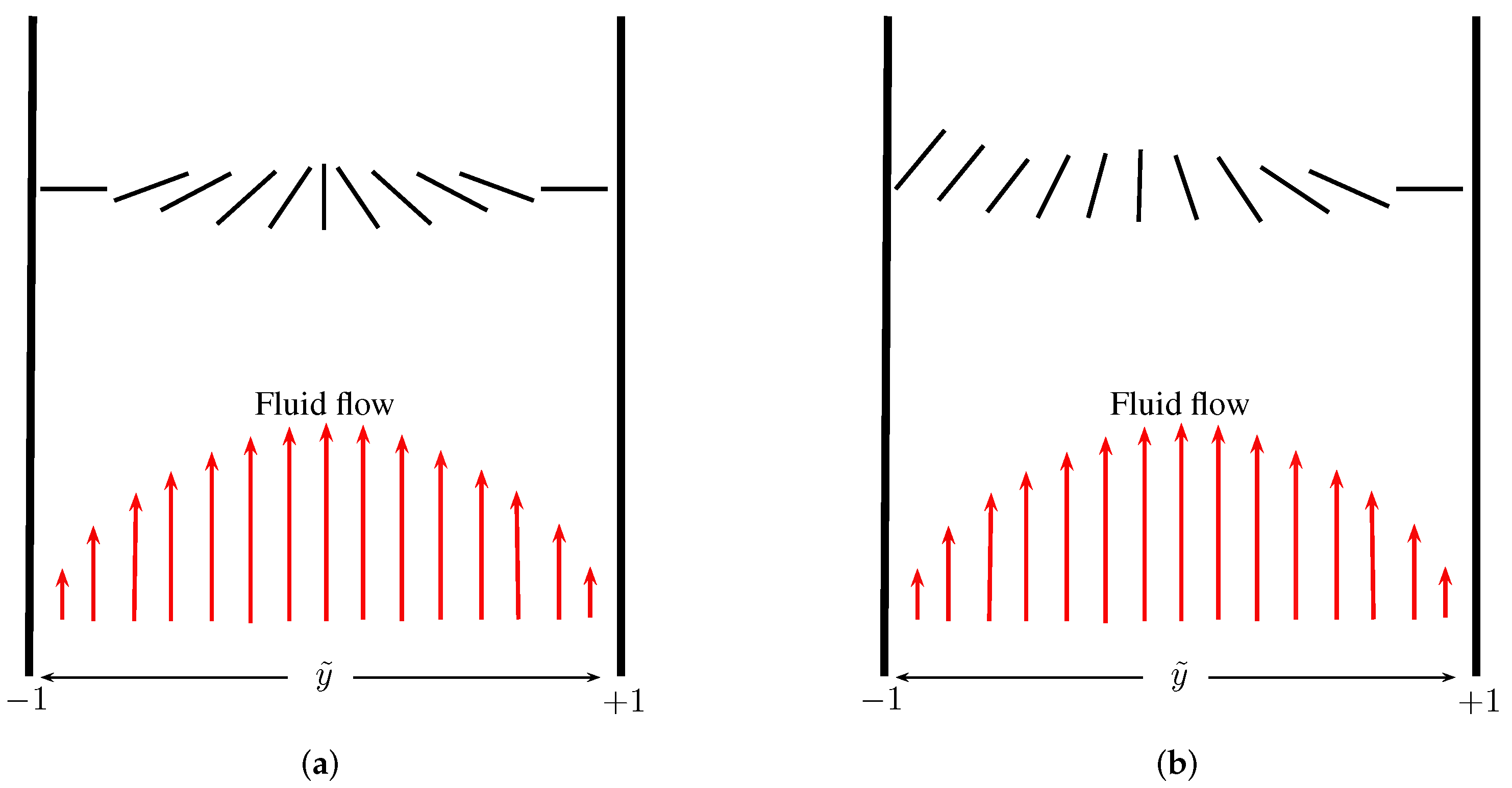
The boundary conditions for $\tilde{s}$ and $\tilde{u}$ are

$$\begin{array}{cc}\hfill \tilde{s}(-1,\tilde{t})=\tilde{s}\left(1,\tilde{t}\right)& =1,\hfill \end{array}$$

(13)

$$\begin{array}{cc}\hfill \tilde{u}\left(-1,\tilde{t}\right)=\tilde{u}\left(1,\tilde{t}\right)& =0.\hfill \end{array}$$

(14)

This simply means that we assume the nematic molecules are perfectly ordered at $\tilde{y}=\pm 1$ and we impose the typical no-slip boundary conditions on $\tilde{y}=\pm 1$. For the nematic director, we look at two different cases: (i) symmetric Dirichlet conditions for $\theta$ on $\tilde{y}=\pm 1$ consistent with strong anchoring and in the spirit of [8], (ii) a Neumann-type boundary condition modelling weak anchoring on $\tilde{y}=-1$ accompanied by a Dirichlet condition on $y=1$ as shown below.

$$\begin{array}{cc}\hfill \mathrm{Symmetric}\text{:}& \theta \left(-1,\tilde{t}\right)=-\omega \pi \mathrm{and}\theta \left(1,\tilde{t}\right)=\omega \pi ,\hfill \end{array}$$

(15)

$$\begin{array}{cc}\hfill \mathrm{Asymmetric}\text{:}& B{\theta }_{\tilde{y}}\left(-1,\tilde{t}\right)-\sin \left[2\theta \left(-1,\tilde{t}\right)\right]=0\mathrm{and}\theta \left(1,\tilde{t}\right)=\omega \pi ,\hfill \end{array}$$

(16)

where

$$\begin{array}{c}\hfill \omega =\frac{\theta (1,\tilde{t})-\theta (-1,\tilde{t})}{2\pi }\end{array}$$

(17)

is the winding number and B is a rescaled anchoring strength (see Figure 1 for a sketch of these configurations). It is worth pointing out that positive B models tangential or planar boundary conditions on the bottom substrate i.e., it originates from a surface energy of the form $\int A{\sin }^2\theta$ that is minimised by either $\theta =0$ or $\theta =\pi$, for a positive anchoring coefficient A that measures the strength of the anchoring and we integrate over the surface $\tilde{y}=-1$. The initial conditions for the system above Equations (9)–(11) are given by

$$\begin{array}{cc}\hfill \tilde{s}\left(\tilde{y},0\right)& =1,\hfill \end{array}$$

(18)

$$\begin{array}{cc}\hfill \theta \left(\tilde{y},0\right)& =\frac{1}{2}\left(\tilde{y}-1\right)\left[\omega \pi -\theta (-1,0)\right]+\omega \pi ,\hfill \end{array}$$

(19)

$$\begin{array}{cc}\hfill \tilde{u}\left(\tilde{y},0\right)& =-\frac{{\tilde{p}}_x}{2}\left(1-{\tilde{y}}^2\right),\hfill \end{array}$$

(20)

where $\theta \left(-1,0\right)$ is the root of the equation $B\theta \left(-1,0\right)-\sin \left[2\theta \left(-1,0\right)\right]=0$ for the asymmetric case.

We will often make comparisons between situations with no flow to situations with fluid flow. In the no-flow case, we simply set $\tilde{u}(\tilde{y},\tilde{t})=0$ in Equations (9) and (10) and analyse the resulting system

$$\begin{array}{cc}\hfill {\tilde{s}}_{\tilde{t}}-{\tilde{s}}_{\tilde{y}\tilde{y}}& =-4\tilde{s}{\theta }_{\tilde{y}}^2-\frac{\tilde{s}}{L^{\ast }}\left({\tilde{s}}^2-1\right),\hfill \end{array}$$

(21)

$$\begin{array}{cc}\hfill {\theta }_{\tilde{t}}-{\theta }_{\tilde{y}\tilde{y}}& =\frac{2}{\tilde{s}}{\tilde{s}}_{\tilde{y}}{\theta }_{\tilde{y}},\hfill \end{array}$$

(22)

with the same boundary (Equations (13), (15) and (16)) and initial conditions (Equations (18) and (19)).

3. Results

The numerical computations are carried out using the finite-element-based commercial package COMSOL v5.2 [30]. Recent numerical work shows that the system (9)–(11) subject to the boundary conditions (13), (14) and either (15) or (16) along with initial conditions (18)–(20) has multiple solutions, which can be interpreted as multiple steady-state solutions or locally stable states for the long-time dynamics. Hence, our numerical results are not exhaustive but serve to illustrate interesting solutions that can be attained under certain model situations, particularly with reference to flow-reversal solutions for the velocity profiles.

3.1. Comparison of the Flow and No–Flow Situation

We neglect time dependence or transient dynamics in this section and focus on the long-time equilibrium profiles of $\tilde{s},\tilde{u}$ and $\theta$ in this section. We fix the parameters $L^{\ast }={10}^{-3}$ and $L_1={10}^{-6}$, which are physically relevant values from the typical values of material constants reported in the literature and investigate the effects of the parameters, ${\tilde{p}}_x$ and $L_2$ on the solution profiles for Equations (9)–(11) [9,24]. The results are presented in Figure 2 and Figure 3 where we plot the no-flow profiles for $\tilde{s}$ and $\theta$ for reference and then compare these profiles to the distorted profiles with a non-zero pressure gradient ${\tilde{p}}_x$. In Figure 2, we study the effect of the ratio ${\tilde{p}}_x/L_2$ on the spatial profiles of $\tilde{s},\tilde{u}$ and $\theta$ with the symmetric Dirichlet boundary conditions, (Equation (15)). Here, the solution profiles are symmetric around $\tilde{y}=0$ due to the imposed symmetry of the boundary conditions. For $L_2/\left|{\tilde{p}}_x\right|\ll 1$, it is relatively straightforward to see that the flow profile is simply the parabolic Poiseuille form. We confirm this observation in Section 4, where we determine the precise form of $\tilde{u}$, along with $\tilde{s}$ and $\theta$, via a systematic asymptotic analysis of the set-up in the limit $L_2/\left|{\tilde{p}}_x\right|\ll 1$. For very small values of ${\tilde{p}}_x$, the flow is weak as expected. In Figure 3, we do the same for asymmetric boundary conditions (Equation (16)). Naturally, the profiles of $\theta$ are not symmetric around $\tilde{y}=0$ in this case. The asymmetric behaviour in $\theta$ is weak, but more pronounced for larger values of $L_2$. The profiles of $\tilde{s}$ and $\tilde{u}$ are largely unaffected by the asymmetric boundary conditions for $\theta$, at least for the parameter values employed in this section.

Further, we can also compute the total fluid flow rate

$$\begin{array}{c}\hfill {\int }_{-1}^1\tilde{u}\mathrm{d}\tilde{y},\end{array}$$

(23)

as well as the wall shear stress,

$${\tilde{\tau }}_w={\left[\frac{\partial \tilde{u}}{\partial \tilde{y}}\right]}_{\tilde{y}=-1},$$

(24)

which is related to the skin friction coefficient, $C_s$, by

$$C_s=\frac{2{\tau }_w}{\rho u_0^2}=\frac{2{\tilde{\tau }}_w}{L_{1}E{r}^{\ast 2}}.$$

(25)

The skin friction coefficient represents the friction drag exerted by the wall, which resists the fluid movement.

In Figure 4, we plot the total volumetric flow rate as a function of $L_2$ for two different values of ${\tilde{p}}_x=\pm 1$, Dirichlet conditions on $\tilde{y}=\pm 1$ and two different values of B. The results suggest that, for $L_2\ge 1$, the net flow rate is greater for ${\tilde{p}}_x=-1$ compared to ${\tilde{p}}_x=1$. This is the richest regime where both the pressure gradient and the liquid crystal parameter $L_2$ influence fluid flow and it would be interesting to investigate how $p_x$ and $L_2$ couple together in fluid flow profiles. Moreover, the effect of the wall-alignment constant B on the flow properties can be inferred from Figure 4. This suggests that by altering the wall-anchoring properties (manifested through B) one can manipulate the flow rate and the skin-friction losses. For example, positive B corresponds to preferred tangential anchoring on $\tilde{y}=-1$ and negative B indicates preferred normal/homeotropic boundary conditions on $\tilde{y}=-1$. Since $\theta =\frac{\pi }{2}$ on $\tilde{y}=1$ ($\omega =\frac{1}{2}$), we have homeotropic boundary conditions on $\tilde{y}=1$. These results suggest that the net flow rate and the wall shear stress are enhanced by Dirichlet conditions or mixed tangential conditions on $\tilde{y}=-1$ along with normal boundary conditions on $\tilde{y}=1$. We emphasise that the wall shear stress ${\tilde{\tau }}_w$ is computed on $\tilde{y}=-1$ where the mixed boundary condition is imposed and the other boundary wall will have a different magnitude (or even direction) of ${\tilde{\tau }}_w$ associated with it.

A phase-space plot of the parameters that correspond to net zero flow rate is shown in Figure 5, also demonstrating the effect of the wall anchoring conditions. For illustrative purposes, we take ${\tilde{p}}_x=1$. The combination of parameters in the region below the curves in Figure 5 corresponds to fluid flow in the direction of decreasing hydrodynamic pressure, while the region above the curves is in the direction of increasing hydrodynamic pressure, which is a manifestation of backflow. A similar situation, in which a net zero fluid flow rate can be observed, is in electro-osmotic flows, for a critical electrical field strength that exactly balances the hydrodynamic driving pressure [31]. The results in Figure 5 provide quantitative estimates for the onset of flow reversal for a specific choice of parameters. A more exhaustive study on these lines can predict the onset of flow reversal for experimentally relevant or applications-oriented modelling scenarios and flow reversal or tunable flow directions offer new possibilities for topological defects and transport phenomena in microfluidic channels. We do not explore this further in this manuscript.

3.2. Effect of the Winding Number $\omega$

The impact of the winding number $\omega$ on the long-time profiles for the symmetric (Equation (15)) and asymmetric case (using Equation (16)) respectively, are shown in Figure 6 and Figure 7 for $L^{\ast }={10}^{-3}$. As $\omega$ increases, the energetic penalties for distortions in $\theta$ increases (this can be seen by re-scaling $\theta =\omega \tilde{\theta }$ in Equation (9)), so the long-time $\theta$-profiles become more linear as $\omega$ increases. The gradient ${\theta }_{\tilde{y}}$ is usually maximum in magnitude at $\tilde{y}=0$ and consequently, $\tilde{s}$ is a minimum at $\tilde{y}=0$ since the energetic penalty is proportional to ${\tilde{s}}^2$. Further, the minimum value of $\tilde{s}$ decreases as $\omega$ increases, again for similar reasons in the sense that the order decreases to compensate for more distortion in the $\theta$ profiles. It is interesting that the total flow rate decreases as $\omega$ increases since the flow meets greater resistance from the increasingly distorted $\theta$ profiles. It seems difficult to extract this behaviour from a simple analysis of the governing partial differential equations.

3.3. Effect of the Parameter $L^{\ast }$

The regime of small $L^{\ast }$ is well understood in the no-flow case. Here, $\tilde{s}$ is approximately unity everywhere and $\theta$ is linear with Dirichlet boundary conditions without flow. When a pressure gradient is imposed, one can perform heuristic calculations to predict that the flow profile is approximately parabolic for small $L_2$, as in Figure 8c and Figure 9c. (See Section 4 for a more detailed analysis). In the case of symmetric Dirichlet boundary conditions, as $L^{\ast }$ becomes larger, $\theta$ becomes approximately constant everywhere except for a jump at $\tilde{y}=0$ to enable the boundary conditions to be satisfied. This can be seen from Equation (9) that as $L^{\ast }$ increases, ${\theta }_{\tilde{y}}$ tends to zero almost everywhere and there is reduced energetic penalty associated with deviations from $\tilde{s}=1$. In fact, $\tilde{s}=0$ when $\theta$ has a jump discontinuity, to regularise the solution. This is referred to as order reconstruction in the liquid-crystal literature when the system interpolates between two fixed boundary conditions by not rotating the eigenframe but by switching the leading eigenvalue at the centre of the cell. However, whilst the order-reconstruction phenomenon is relatively well understood without flow effects, it is far less studied with flow effects. We make certain observations here. For the parameter choices in Figure 8, the $\theta$ profile switches from a continuous solution to a discontinuous solution at $\tilde{y}=0$ at $L^{\ast }\approx 0.1$. This has a very interesting effect on the flow profile (see Figure 8c) in the sense that there is a distinct region in the channel interior where $\tilde{u}<0$ for $L^{\ast }=0.1$ and the flow field has a cusp-like minimum at $\tilde{y}=0$. For larger values of $L^{\ast }$, when the system has settled into the order-reconstruction regime, the flow profiles are less surprising and have the usual parabolic-like form. We point out that $\theta$ is not a constant on either side of the jump discontinuity for order reconstruction with flow, in contrast to order reconstruction without flow. The qualitative features are unchanged with asymmetric boundary conditions, see the results in Figure 9c.

For a select range of values of $L^{\ast }$, both the continuous and discontinuous solutions for $\theta$ are attainable, with the state achieved dependent on the initial condition. We analyse this further in Section 3.5.

There is evidence that the local fluid flow switches direction (at least locally) for certain choices of $L^{\ast }$ and we have investigated the impact of $L^{\ast }$ on the net fluid flow rate, as shown in Figure 10. As we have seen in Figure 5, for a given $L_2$ large enough, there exists a critical $L^{\ast }$ ($L_{crit,1}^{\ast }$) for which there is zero net flow. However, here we find that there is a second critical $L^{\ast }$ ($L_{crit,2}^{\ast }$), beyond which the flow switches back to the direction of the decreasing pressure. The critical scaled elastic constants $L_{crit,1}^{\ast }$ and $L_{crit,2}^{\ast }$ have almost the same values for both the symmetric and asymmetric boundary conditions, for the parameter choices in Figure 10. The critical values are relatively large however, and hence unlikely to be attained in most applications.

3.4. Dynamic Evolution of the Spatial Profiles

We briefly examine the dynamic evolution of the director profile, order parameter and the fluid flow profiles in Figure 11 (symmetric case) and Figure 12 (asymmetric case). We note that, even though $L_1\ll 1$ in our simulations, the velocity is time dependent because $\tilde{s}$ and $\theta$ are time dependent. The dynamics are not particularly interesting for this choice of parameters but illustrate how $\tilde{s}$ assumes a U-shaped profile with a shallow minimum as $\theta$ evolves from the perfectly linear initial condition, under the effect of flow. The initial flow profile is Poiseuille and the nematic effects suppress the flow profile and distort the parabolic shape.

3.5. Effect of the Initial Condition

Next, we make some preliminary comments on the effect of the initial condition on the equilibrium solution. As noted in Section 3.3, as we increase the parameter $L^{\ast }$, the $\theta$ solution transitions from a continuous to a discontinuous profile, at a critical value of $L^{\ast }$ referred to as $L_{switch}^{\ast }$. This motivates the question of whether, by an appropriate choice of initial condition, there are parameter regimes that admit multiple steady-state solutions with a basin of attraction.

In Figure 13, we consider a specific case of no fluid flow and symmetric Dirichlet boundary conditions in $\theta$ (Equation (15)) and show that the system can indeed exist in multiple steady states.

We find that there is a window of values of $L^{\ast }<L_{switch}^{\ast }\approx 0.0335$ for $\omega =1/2$ (and $L_{switch}^{\ast }$ decreases as we increase $\omega$) for which a continuous and discontinuous steady-state solution can be achieved, depending on the initial conditions, indicating that multiple steady states may only be possible in some parameter regimes. The continuous solution is stable in this parameter regime and the discontinuous solution is unstable with respect to perturbations near the centre of the cell. This is consistent with theoretical work in the field. The order-reconstruction or discontinuous solution exists for all values of $L^{\ast }$, for our choice of symmetric Dirichlet conditions, with no flow. It is the unique solution for suitably large $L^{\ast }$ and unstable for suitably small $L^{\ast }$ [18]. However, the instability only manifests in certain directions, so that, for an appropriate choice of initial condition, we can recover the discontinuous solution for smaller values of $L^{\ast }$. As $L^{\ast }$ increases, we recover the order-reconstruction or discontinuous solution for all initial conditions. These results are promising in the context of bistable devices, particularly if the order-reconstruction or discontinuous solution can be “stabilised” by an appropriate control and we have two stable solutions—the continuous and the discontinuous solution for small values of $L^{\ast }$.

4. Steady-State Analysis

In this section, we analytically study the system Equations (9)–(11) in steady state. We assume that $L_2/\left|{\tilde{p}}_x\right|\ll 1$ so that the flow affects the nematic orientational ordering but not vice versa, and that a uniform pressure gradient ${\tilde{p}}_{\tilde{x}}=-G$ is applied. In particular, this regime does not capture backflow where the nematic order affects fluid flow.

We integrate Equation (11) with respect to $\tilde{y}$ twice and apply boundary conditions (14) to give the following leading-order Poiseuille-type solution for $\tilde{u}$,

$$\begin{array}{c}\hfill \tilde{u}=-\frac{G}{2}\left({\tilde{y}}^2-1\right).\end{array}$$

(26)

Substituting Equation (26) into Equation ((10)) and rearranging we obtain

$$\begin{array}{c}\hfill {\left({\tilde{s}}^2{\theta }_{\tilde{y}}\right)}_{\tilde{y}}=-G\tilde{y}{\tilde{s}}^2.\end{array}$$

(27)

We are thus left to solve Equations (9) and (27), subject to Equation (13), and either Equation (15) or Equation (16).

The numerics have uncovered the possibility for two types of steady solution: continuous or discontinuous solutions in $\theta$. We will study each of these in turn in the following subsections.

4.1. Continuous Solutions in $\theta$

We first study the symmetric strong-anchoring regime or Dirichlet boundary conditions for $\theta$. Integrating Equation (27) with respect to $\tilde{y}$ twice and applying the boundary conditions (15) gives an explicit expression for $\theta$ in terms of $\tilde{s}$:

$$\begin{array}{c}\hfill \theta =-G{\int }_0^{\tilde{y}}\frac{\mathrm{d}\eta }{\tilde{s}{\left(\eta \right)}^2}{\int }_0^{\eta }\zeta \tilde{s}{\left(\zeta \right)}^2\mathrm{d}\zeta +c_1{\int }_0^{\tilde{y}}\frac{\mathrm{d}\eta }{\tilde{s}{\left(\eta \right)}^2},\end{array}$$

(28)

where

$$\begin{array}{c}\hfill {\displaystyle c_1=\frac{{\displaystyle \omega \pi +G{\int }_0^1\frac{\mathrm{d}\eta }{\tilde{s}{\left(\eta \right)}^2}{\int }_0^{\eta }\zeta \tilde{s}{\left(\zeta \right)}^2\mathrm{d}\zeta }}{{\displaystyle {\int }_0^1\frac{\mathrm{d}\eta }{s{\left(\eta \right)}^2}}}.}\end{array}$$

(29)

Substituting for ${\theta }_{\tilde{y}}$ in Equation (9) using Equation (28), we obtain the integro-differential equation for $\tilde{s}$,

$$\begin{array}{c}\hfill {\tilde{s}}_{\tilde{y}\tilde{y}}=4\tilde{s}{\left(-\frac{G}{{\tilde{s}}^2}{\int }_0^{\tilde{y}}\eta \tilde{s}{\left(\eta \right)}^2\mathrm{d}\eta +\frac{c_1}{{\tilde{s}}^2}\right)}^2+\frac{\tilde{s}}{L^{\ast }}({\tilde{s}}^2-1).\end{array}$$

(30)

This must be solved subject to the boundary conditions (13). An analogous procedure follows for the asymmetric anchoring conditions (Equation (16)), but we do not present the details here.

Small-$L^{\ast }$ Limit

It is observed that continuous solutions are stable for $L^{\ast }\ll 1$. We thus explore the system in this reduced regime. In this case, the leading-order solution in $L^{\ast }$ to Equation (30) can immediately be seen to be $\tilde{s}=1$. As a result, Equation (28) yields the corresponding leading-order solution for $\theta$,

$$\begin{array}{c}\hfill \theta =-\frac{G{\tilde{y}}^3}{6}+\left(\omega \pi +\frac{G}{6}\right)\tilde{y}.\end{array}$$

(31)

A similar method in the asymmetric case, Equation (28), yields the leading-order solution

$$\begin{array}{c}\hfill \theta =-\frac{G}{6}(y^3-1)+c_2(y-1)+\omega \pi ,\end{array}$$

(32)

with $c_2$ satisfying the transcendental equation

$$\begin{array}{c}\hfill \left(\frac{G}{2}+c_2\right)B=\sin \left[\frac{2G}{3}-4c_2+2\omega \pi \right].\end{array}$$

(33)

We note also that in the small-$L^{\ast }$ limit, we may relax the assumption that $L_2$ is small. In this case, the flow profile is still parabolic to leading order, but is given by

$$\begin{array}{c}\hfill \tilde{u}=-\frac{G}{2(1-L_2)}\left({\tilde{y}}^2-1\right).\end{array}$$

(34)

We recall that $L_2>0$ is positive since we are working with low temperatures, so $a>0$. Negative values of $L_2$ describe higher temperatures for which $\tilde{s}\approx 1$ does not hold. We also note that the flow profiles in the preceding section do not agree with the perfectly parabolic profile described above. This is largely because $L^{\ast }$ is not sufficiently small in the simulations for the sake of computational efficiency.

4.2. Discontinuous Solutions in $\theta$

We now study the case to allow for discontinuities in $\theta$. On physical grounds, $\tilde{s}=0$ vanishes at such discontinuities to "regularise" the discontinuities. While such point discontinuities may appear anywhere within the domain, for illustrative purposes we consider the case where a single point discontinuity in $\theta$ is present, at $\tilde{y}=0$. We focus on the symmetric strong-anchoring regime, but again note that similar methods apply to the asymmetric boundary conditions. We solve in the domain $0<\tilde{y}\le 1$ and replace the boundary conditions (Equations (13) and (15)) with

$$\begin{array}{cccc}\hfill \tilde{s}(0,\tilde{t})& =0,\hfill & \hfill \tilde{s}\left(1,\tilde{t}\right)& =1,\hfill \end{array}$$

(35)

$$\begin{array}{cccc}\hfill {\theta }_{\tilde{y}}(0^{+},\tilde{t})& =\mathrm{finite},\hfill & \hfill \theta (1,\tilde{t})& =\omega \pi .\hfill \end{array}$$

(36)

Since $L_2\ll 1$, the velocity profile is not influenced by the discontinuities and is still given by Equation (26).

Integrating Equation (27) and applying the modified boundary conditions, we find that $\theta$ is now given by

$$\begin{array}{c}\hfill \theta =\omega \pi +G{\int }_{\tilde{y}}^1\frac{\mathrm{d}\eta }{\tilde{s}{\left(\eta \right)}^2}{\int }_0^{\eta }\zeta \tilde{s}{\left(\zeta \right)}^2\mathrm{d}\zeta .\end{array}$$

(37)

Substituting for $\theta$ in Equation (37) into Equation (9) yields

$$\begin{array}{c}\hfill {\tilde{s}}_{\tilde{y}\tilde{y}}=\frac{4G^2}{{\tilde{s}}^3}{\left({\int }_0^{\tilde{y}}\eta \tilde{s}{\left(\eta \right)}^2\mathrm{d}\eta \right)}^2+\frac{\tilde{s}}{L^{\ast }}({\tilde{s}}^2-1),\end{array}$$

(38)

subject to Equation (35).

When there is no external flow, ${\tilde{p}}_x=G=0$ and Equation (37) gives simply $\theta =\omega \pi$. The solution for $\tilde{s}$ is then given implicitly from Equation (30) as

$$\begin{array}{c}\hfill \tilde{y}=\sqrt{2L^{\ast }}{\int }_0^{\tilde{s}}\frac{\mathrm{d}\eta }{\sqrt{{\eta }^4-2{\eta }^2+c_3}},\end{array}$$

(39)

where $c_3$ is given by

$$\begin{array}{c}\hfill \sqrt{2L^{\ast }}{\int }_0^1\frac{\mathrm{d}\eta }{\sqrt{{\eta }^4-2{\eta }^2+c_3}}=1,\end{array}$$

(40)

for a given $L^{\ast }$. Note that, equivalently, Equation (40) could be viewed as providing explicitly the value of $L^{\ast }$ corresponding to a particular chosen value of $c_3$. The solution for $-1\le \tilde{y}<0$ is found by an odd reflection of the solution in $0<\tilde{y}\le 1$.

When the pressure gradient $G\ll 1$, the system possesses a distinguished limit when $L^{\ast }=O(1/G^2)$. (Note we assume that $L_2\ll G$ so that the second term on the right-hand side of Equation (11) can still be ignored). In this relatively simple case, the equations are amenable to asymptotic analysis, and we are able to write the solution for $\tilde{s}$ and $\theta$ explicitly as

$$\begin{array}{cc}\hfill \tilde{s}& =\tilde{y}+\frac{G^2\tilde{y}}{168}({\tilde{y}}^6-1)+\frac{\tilde{y}}{20L^{\ast }}({\tilde{y}}^4-1)-\frac{\tilde{y}}{6L^{\ast }}({\tilde{y}}^2-1)+O\left(G^4\right),\hfill \end{array}$$

(41)

$$\begin{array}{cc}\hfill \theta & =\omega \pi +\frac{G}{12}\left({\tilde{y}}^3-1\right)+O\left(G^2\right).\hfill \end{array}$$

(42)

5. Conclusions

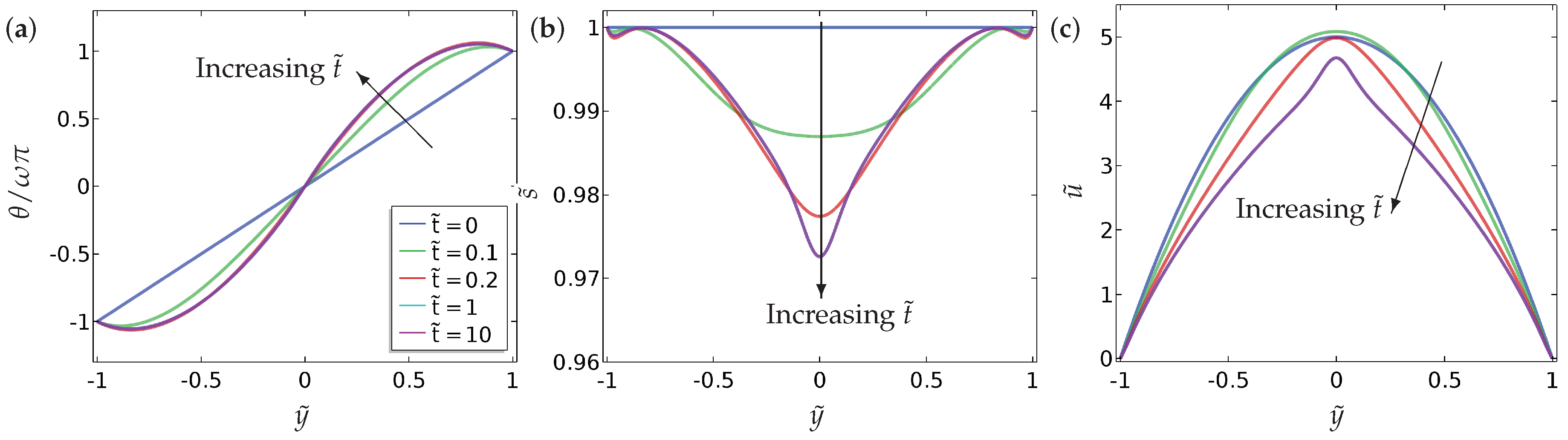
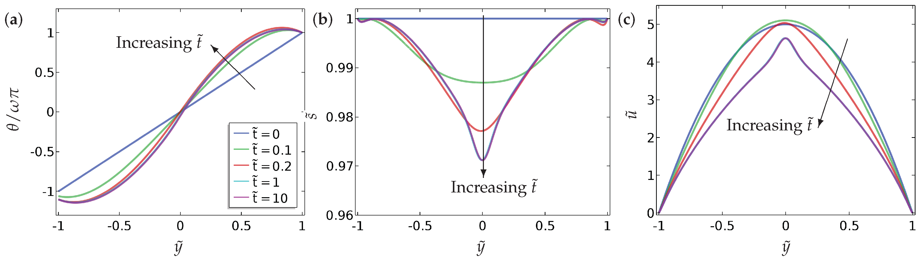
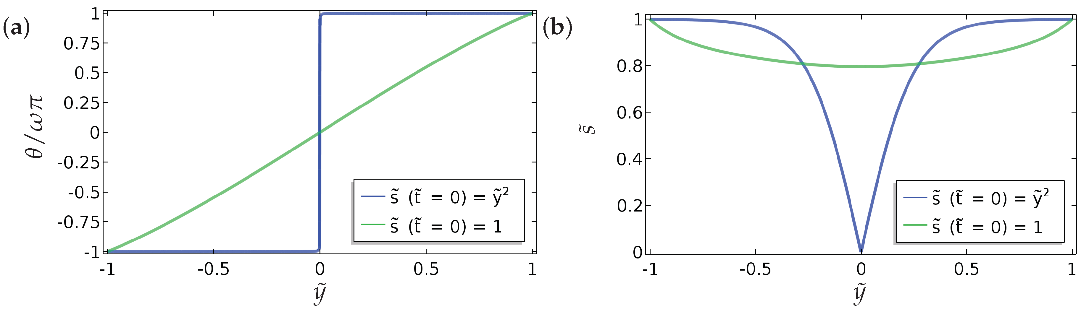
In this paper, we investigate the nematic order parameter (captured by the director orientation $\theta$ and the order parameter $\tilde{s}$) and flow profiles in a one-dimensional microfluidic channel, with Dirichlet boundary conditions and mixed boundary conditions for $\theta$, as a function of the pressure gradient, the boundary conditions themselves (in terms of winding number $\omega$ and a measure of the anchoring strength B), the nematic elastic constant ($L^{\ast }$) and the scaled viscosities ($L_2$) in a reduced Beris–Edwards setting. For small $L_2$, we can analyse the system and obtain at least semi-explicit solutions for the nematic order parameter and the flow profile, both with and without an applied pressure gradient. We consider continuous and discontinuous profiles for $\theta$ separately, again including the effect of the pressure gradient. In the discontinuous case, $\theta$ is effectively piecewise constant (without flow) for such solutions and discontinuities in $\theta$ are regularised by isotropic points with $\tilde{s}=0$. We can analytically construct solutions with multiple discontinuities although we suspect that these solutions lose stability with respect to higher-dimensional perturbations. The analytical results set the scene for some interesting control problems on how to stabilise discontinuous solutions for small $L^{\ast }$ and these discontinuous solutions could offer interesting examples of domain walls with $\tilde{s}=0$ in three dimensions.

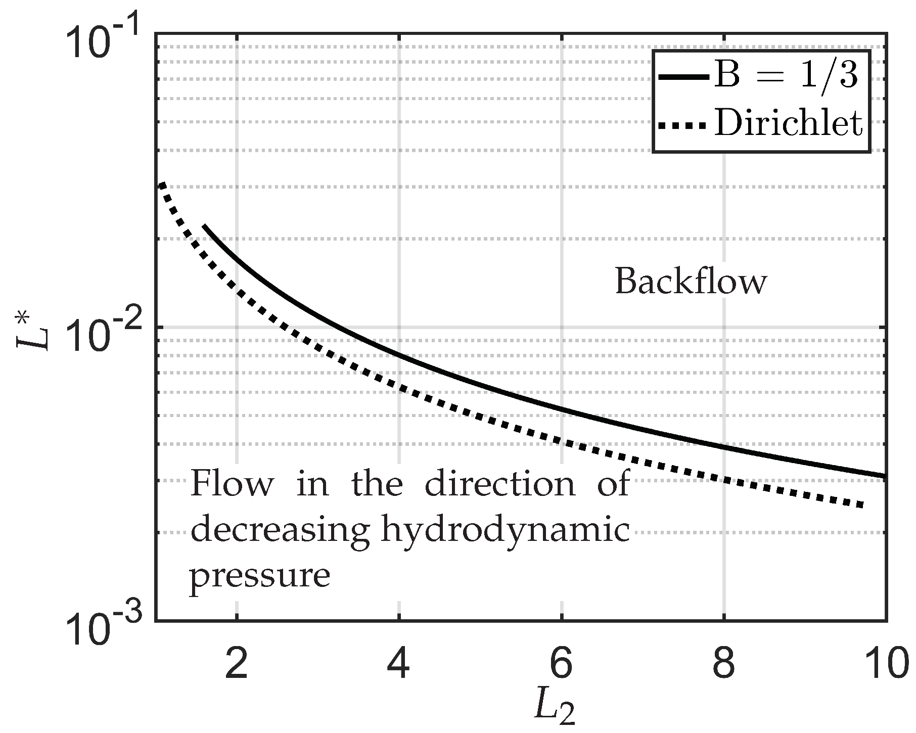
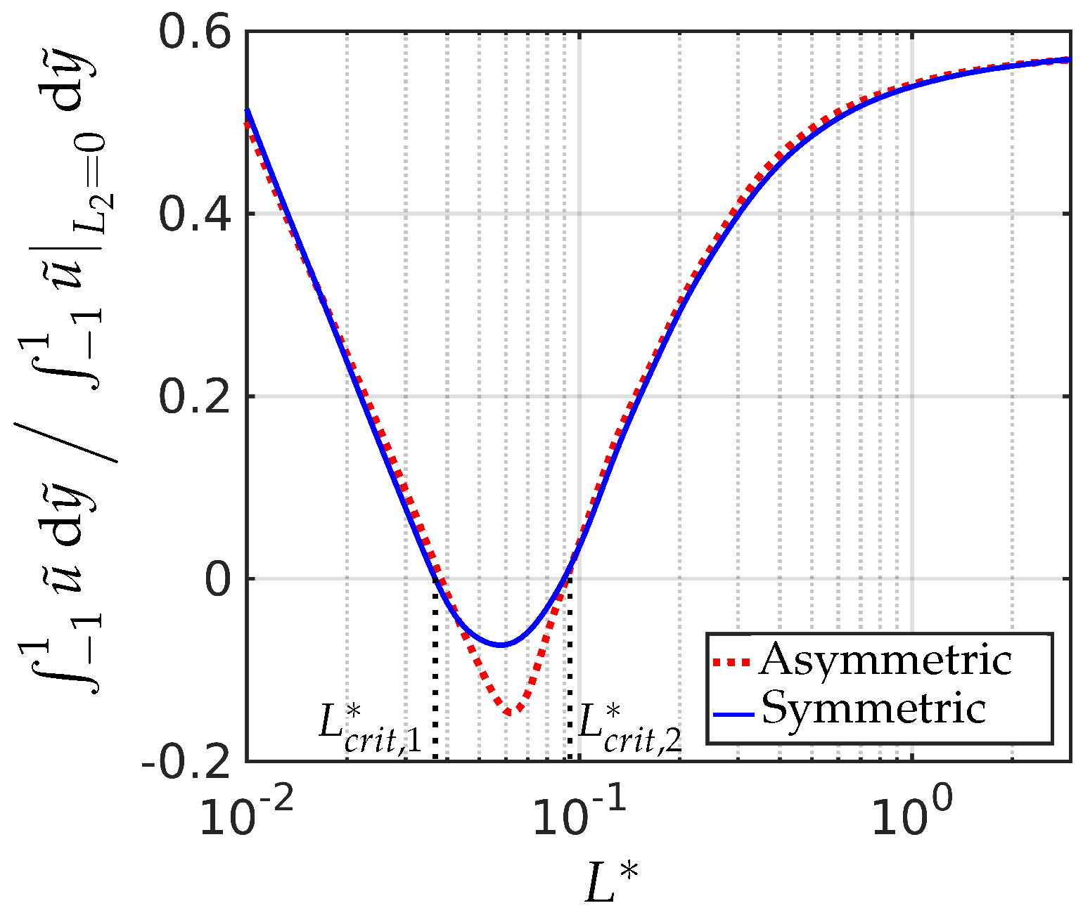
Our most interesting observations include the onset of flow reversal in these model microfluidic systems. We compute specific criteria for flow reversal (flow in the direction of the pressure gradient) as a function of $L^{\ast }$ and $L_2$ and in particular, based on the results in Figure 10, we expect the curve in Figure 5 to fold back on itself, so that for a given $L_2$ large enough, flow reversal only occurs for a certain range of values $L^{\ast }$ and not in the entire region above the dotted and solid curves in Figure 5. The observed flow reversal is a distinct manifestation of backflow and only occurs for large enough $L_2$. We plan to investigate discontinuous order-reconstruction solutions in the presence of flow and backflow in microfluidic channels as a function of temperature (treating a as a parameter or accounting for cases when $L_2$ changes sign), geometrical dimensions and the anchoring coefficient B in subsequent work.

References

1. De Gennes, P.-G.; Prost, J. The Physics of Liquid Crystals (International Series of Monographs On Physics); Oxford University Press: Cary, NC, USA, 1995. [Google Scholar]
2. Brochard, F. Backflow Effects in Nematic Liquid Crystals. Mol. Cryst. Liquid Cryst. 1973, 23, 51–58. [Google Scholar] [CrossRef]
3. Mieda, Y.; Furutani, K. Micromanipulation method using backflow effect of liquid crystals. In Proceedings of the 2006 International Symposium on Micro-NanoMechatronics and Human Science, Nagoya, Japan, 5–8 November 2006; pp. 1–6. [Google Scholar]
4. Vanbrabant, P.J.M.; Beeckman, J.; Neyts, K.; James, R.; Fernandez, F.A. Effect of material properties on reverse flow in nematic liquid crystal devices with homeotropic alignment. Appl. Phys. Lett. 2009, 95, 151108. [Google Scholar] [CrossRef] [Green Version]
5. Leslie, F.M. Some constitutive equations for liquid crystals. Arch. Ration. Mech. Anal. 1968, 28, 265–283. [Google Scholar] [CrossRef]
6. Ericksen, J.L. Equilibrium theory of liquid crystals. In Advances in Liquid Crystals; Elsevier: New York, NY, USA, 1976; Volume 2, pp. 233–298. [Google Scholar]
7. Beris, A.N.; Edwards, B.J. Thermodynamics of Flowing Systems: With Internal Microstructure; Number 36; Oxford University Press: Oxford, UK, 1994. [Google Scholar]
8. Crespo, M.; Majumdar, A.; Ramos, A.M.; Griffiths, I.M. Solution landscapes in nematic microfluidics. Phys. D Nonlinear Phenom. 2017, 351, 1–13. [Google Scholar] [CrossRef]
9. Majumdar, A.; Zarnescu, A. Landau-de Gennes theory of nematic liquid crystals: The Oseen–Frank limit and beyond. Arch. Ration. Mech. Anal. 2010, 196, 227–280. [Google Scholar] [CrossRef]
10. Tóth, G.; Denniston, C.; Yeomans, J.M. Hydrodynamics of topological defects in nematic liquid crystals. Phys. Rev. Lett. 2002, 88, 105504. [Google Scholar] [CrossRef] [PubMed]
11. Chen, G.-Q.; Majumdar, A.; Wang, D.; Zhang, R. Global existence and regularity of solutions for active liquid crystals. J. Differ. Equat. 2017, 263, 202–239. [Google Scholar] [CrossRef] [Green Version]
12. Denniston, C.; Orlandini, E.; Yeomans, J.M. Lattice Boltzmann simulations of liquid crystal hydrodynamics. Phys. Rev. E 2001, 63, 056702. [Google Scholar] [CrossRef] [PubMed]
13. Sonnet, A.M.; Maffettone, P.L.; Virga, E.G. Continuum theory for nematic liquid crystals with tensorial order. J. Non-Newtonian Fluid Mech. 2004, 119, 51–59. [Google Scholar] [CrossRef]
14. Xiao, Y. Global strong solution to the three-dimensional liquid crystal flows of Q-tensor model. J. Differ. Equat. 2017, 262, 1291–1316. [Google Scholar] [CrossRef] [Green Version]
15. Luo, C.; Majumdar, A.; Erban, R. Multistability in planar liquid crystal wells. Phys. Rev. E 2012, 85, 061702. [Google Scholar] [CrossRef] [PubMed]
16. Kusumaatmaja, H.; Majumdar, A. Free energy pathways of a multistable liquid crystal device. Soft Matter 2015, 11, 4809–4817. [Google Scholar] [CrossRef] [PubMed] [Green Version]
17. Canevari, G.; Majumdar, A.; Spicer, A. Order reconstruction for nematics on squares and hexagons: A Landau–de Gennes study. SIAM J. Appl. Math. 2017, 77, 267–293. [Google Scholar] [CrossRef]
18. Bisi, F.; Gartland, E.C., Jr.; Rosso, R.; Virga, E.G. Order reconstruction in frustrated nematic twist cells. Phys. Rev. E 2003, 68, 021707. [Google Scholar] [CrossRef] [PubMed]
19. Lin, F.H.; Liu, C. Static and dynamic theories of liquid crystals. J. Partial Differ. Equat. 2001, 14, 289–330. [Google Scholar]
20. Biscari, P.; Sluckin, T.J. A perturbative approach to the backflow dynamics of nematic defects. Eur. J. Appl. Math. 2012, 23, 181–200. [Google Scholar] [CrossRef]
21. Marenduzzo, D.; Orlandini, E.; Yeomans, J.M. Hydrodynamics and rheology of active liquid crystals: A numerical investigation. Phys. Rev. Lett. 2007, 98, 118102. [Google Scholar] [CrossRef] [PubMed]
22. Blanc, C.; Svenšek, D.; Žumer, S.; Nobili, M. Dynamics of nematic liquid crystal disclinations: The role of the backflow. Phys. Rev. Lett. 2005, 95, 1–4. [Google Scholar] [CrossRef] [PubMed]
23. Paicu, M.; Zarnescu, A. Energy dissipation and regularity for a coupled Navier–Stokes and q-tensor system. Arch. Ration. Mech. Anal. 2012, 203, 45–67. [Google Scholar] [CrossRef]
24. Sengupta, A.; Tkalec, U.; Ravnik, M.; Yeomans, J.M.; Bahr, C.; Herminghaus, S. Liquid crystal microfluidics for tunable flow shaping. Phys. Rev. Lett. 2013, 110, 048303. [Google Scholar] [CrossRef] [PubMed]
25. Mondal, S.; Majumdar, A.; Griffiths, I.M. Nematohydrodynamics for Colloidal Self-Assembly and Transport Phenomena. arXiv, 2017; arXiv:1707.09015. [Google Scholar]
26. Emmrich, E.; Klapp, S.H.; Lasarzik, R. Nonstationary models for liquid crystals: A fresh mathematical perspective. arXiv, 2017; arXiv:1708.06937. [Google Scholar]
27. Wang, W.; Zhang, P.; Zhang, Z. Rigorous derivation from Landau-de Gennes theory to Ericksen–Leslie theory. SIAM J. Math. Anal. 2013, 47, 127–158. [Google Scholar] [CrossRef]
28. Batista, V.M.; Blow, M.L.; Gama, M.M.T. The effect of anchoring on the nematic flow in channels. Soft Matter 2015, 11, 4674–4685. [Google Scholar] [CrossRef] [PubMed] [Green Version]
29. Giomi, L.; Mahadevan, L.; Chakraborty, B.; Hagan, M.F. Banding, excitability and chaos in active nematic suspensions. Nonlinearity 2012, 25, 2245. [Google Scholar] [CrossRef]
30. Pryor, R.W. Multiphysics Modeling Using COMSOL: A First Principles Approach; Jones & Bartlett Publishers: Burlington, MA, USA, 2009. [Google Scholar]
31. Mondal, S.; De, S. Effects of non-Newtonian power law rheology on mass transport of a neutral solute for electro-osmotic flow in a porous microtube. Biomicrofluidics 2013, 7, 044113. [Google Scholar] [CrossRef] [PubMed]
Figure 1. Schematic of the director orientation in equilibrium when applying (a) symmetric anchoring conditions Equation (15) and (b) asymmetric anchoring conditions Equation (16).
Fluids 03 00039 g001
Figure 2. The effect of the fluid flow on (a) the director orientation ( θ ) , (b) the order parameter ( s ˜ ) , and (c) the velocity ( u ˜ ), at equilibrium, for the case of symmetric boundary condition (Equation (15)). The values of the parameters used are ω = 1 / 2 , L = 10 3 and L 1 = 10 6 . (Here, and elsewhere, we plot the profiles at t ˜ = 10 , after which time we find the solutions have relaxed to a steady state from the initial configuration, Equations (18)–(20).) Analytic solutions are given in Section 4 and Section 4.1.
Fluids 03 00039 g002
Figure 3. The effect of the fluid flow on (a) the director orientation ( θ ) , (b) the order parameter ( s ˜ ) , and (c) the velocity u ˜ , at equilibrium ( t ˜ = 10 ) , for the case of asymmetric boundary condition (Equation (16)). The values of the parameters used are B = 1 / 3 , ω = 1 / 2 , L = 10 3 and L 1 = 10 6 .
Fluids 03 00039 g003
Figure 4. Plot of (a) the total volumetric flow rate and (b) the wall shear stress (which relates to the skin friction coefficient through Equation (25)) as a function of L 2 for different values of the constant B in the symmetric (Dirichlet) case, Equation (15), and the asymmetric case, Equation (16), for θ . The total flow rate is scaled with the equivalent Poiseuille flow rate for a Newtonian fluid, 1 1 u ˜ | L 2 = 0 d y ˜ = 2 p ˜ x / 3 . The solid and the dotted lines correspond to the negative and positive values of p ˜ x respectively. The values of the parameters used are | p ˜ x | = 1 , ω = 1 / 2 , L = 10 3 and L 1 = 10 6 1 .
Fluids 03 00039 g004
Figure 5. Phase space plot of the parameters ( L and L 2 ) for no overall mass flow rate. Here p ˜ x > 0 . The curve (solid) corresponding to B = 1 / 3 is for the asymmetric boundary condition (Equation (16)). The dotted curve is for the case of the symmetric (Dirichlet) boundary condition (Equation (15)). The values of the parameters used are p ˜ x = 1 , ω = 1 / 2 and L 1 = 10 6 .
Fluids 03 00039 g005
Figure 6. The effect of the winding number ω on (a) the director orientation ( θ ), (b) the order parameter ( s ˜ ) and (c) the velocity ( u ˜ ), at equilibrium ( t ˜ = 10 ) . In this case, we have considered the symmetric boundary condition in θ (Equation (15)). The values of the parameters used are L = 10 3 , p ˜ x = 10 , L 2 = 1 , and L 1 = 10 6 . The legends of all the sub-figures are the same as in (a).
Fluids 03 00039 g006
Figure 7. The effect of the winding number ω on (a) the director orientation ( θ ), (b) the order parameter ( s ˜ ) and (c) the velocity ( u ˜ ), at equilibrium ( t ˜ = 10 ) . In this case, we have considered the asymmetric boundary condition in θ (Equation (16)). The values of the parameters used are B = 1 / 3 , L = 10 3 , p ˜ x = 10 , L 2 = 1 , and L 1 = 10 6 . The legends of all the sub-figures are the same as in (a).
Fluids 03 00039 g007
Figure 8. The effect of the parameter L on (a) the director orientation ( θ ) , (b) the order parameter ( s ˜ ) and (c) the velocity ( u ˜ ) , at equilibrium ( t ˜ = 10 ) , in the case of the symmetric boundary conditions for θ (Equation (15)). The values of the parameters used are ω = 1 / 2 , L 2 = 1 , p ˜ x = 10 and L 1 = 10 6 . The legends of all the sub-figures are the same as in (a).
Fluids 03 00039 g008
Figure 9. The effect of the parameter L on (a) the director orientation ( θ ) , (b) the order parameter ( s ˜ ) and (c) the velocity ( u ˜ ) , at equilibrium ( t ˜ = 10 ) , in the case of the asymmetric boundary conditions for θ (Equation (16)). The values of the parameters used are ω = 1 / 2 , B = 1 / 3 , L 2 = 1 , p ˜ x = 10 and L 1 = 10 6 . The legends of all the sub-figures are the same as in (a).
Fluids 03 00039 g009
Figure 10. The effect of the parameter L on the net fluid flow rate at equilibrium ( t ˜ = 10 ) , for the asymmetric (Equation (16)) and symmetric case (Equation (15)). The values of the parameters used are B = 1 / 3 , ω = 1 / 2 , L 2 = 1 , p ˜ x = 10 and L 1 = 10 6 . The total flow rate is scaled with the equivalent Poiseuille flow rate, 1 1 u ˜ | L 2 , L 1 = 0 d y ˜ = 2 p ˜ x / 3 .
Fluids 03 00039 g010
Figure 11. The dynamic evolution of (a) the director orientation ( θ ) , (b) the order parameter ( s ˜ ) and (c) the velocity profile ( u ˜ ) for the symmetric case (Equation 15). The values of the parameters used are ω = 1 / 2 , L = 10 3 , L 2 = 10 , p ˜ x = 10 and L 1 = 10 6 . The legends of all the sub-figures are the same as in (a).
Fluids 03 00039 g011
Figure 12. The dynamic evolution of (a) the director orientation ( θ ) , (b) the order parameter ( s ˜ ) and (c) the velocity profile ( u ˜ ) for the asymmetric case (Equation (16)). The values of the parameters used are B = 1 / 3 , ω = 1 / 2 , L = 10 3 , L 2 = 10 , p ˜ x = 10 and L 1 = 10 6 . The profiles of θ are asymmetric (around y ˜ = 0 ) because of the inhomogeneity in the θ boundary conditions (Equation (16)). The legends of all the sub-figures are the same as in (a).
Fluids 03 00039 g012
Figure 13. Equilibrium profiles of (a) the director orientation, θ and (b) the order parameter s ˜ for two different initial conditions for s ˜ and a linear initial profile for θ , without any fluid flow. The blue curves are the equilibrium profiles for θ and s ˜ for s ˜ ( y ˜ , 0 ) = y ˜ 2 and the green curves are the equilibrium profiles for s ˜ ( y ˜ , 0 ) = 1 . We have considered the symmetric condition for θ given by Equation (15). The values of the parameters used are ω = 1 / 2 and L = 0.03 .
Fluids 03 00039 g013