Multiscale Stuart-Landau Emulators: Application to Wind-Driven Ocean Gyres


1
Department of Atmospheric and Oceanic Sciences, University of California, Los Angeles, CA 90095, USA
2
Department of Mathematics, Imperial College London, London SW7 2AZ, UK
*
Author to whom correspondence should be addressed.
Fluids 2018, 3(1), 21; https://doi.org/10.3390/fluids3010021
Submission received: 13 February 2018
/
Revised: 27 February 2018
/
Accepted: 28 February 2018
/
Published: 6 March 2018
(This article belongs to the Special Issue Reduced Order Modeling of Fluid Flows)
Abstract
:The multiscale variability of the ocean circulation due to its nonlinear dynamics remains a big challenge for theoretical understanding and practical ocean modeling. This paper demonstrates how the data-adaptive harmonic (DAH) decomposition and inverse stochastic modeling techniques introduced in (Chekroun and Kondrashov, (2017), Chaos, 27), allow for reproducing with high fidelity the main statistical properties of multiscale variability in a coarse-grained eddy-resolving ocean flow. This fully-data-driven approach relies on extraction of frequency-ranked time-dependent coefficients describing the evolution of spatio-temporal DAH modes (DAHMs) in the oceanic flow data. In turn, the time series of these coefficients are efficiently modeled by a family of low-order stochastic differential equations (SDEs) stacked per frequency, involving a fixed set of predictor functions and a small number of model coefficients. These SDEs take the form of stochastic oscillators, identified as multilayer Stuart–Landau models (MSLMs), and their use is justified by relying on the theory of Ruelle–Pollicott resonances. The good modeling skills shown by the resulting DAH-MSLM emulators demonstrates the feasibility of using a network of stochastic oscillators for the modeling of geophysical turbulence. In a certain sense, the original quasiperiodic Landau view of turbulence, with the amendment of the inclusion of stochasticity, may be well suited to describe turbulence.
1. Introduction
The turbulent oceanic flows consist of complex motions, jets, vortices and waves that co-exist on very different spatio-temporal scales, but also without clear scale separation. Mesoscale oceanic eddies populate nearly all parts of the global ocean and play important roles in maintaining the oceanic general circulation. The most straightforward, but also the most computationally intensive and, thus, unfeasible, way of accounting for the eddy effects on the large-scale circulation is resolving them dynamically with eddy-resolving ocean general circulation models (GCMs). This brute-force approach requires a computational grid resolution of about 1 km, which makes it feasible only for relatively short time simulations, whereas the Earth system and climate change modeling routinely require much longer simulations over centuries and millennia. One way to afford these time scales, while simulating the ocean in a qualitatively correct way, is to parameterize the important eddy effects with simple and affordable, but still accurate models embedded in the prognostic ocean circulation models.
Thus, the search for suitable eddy parameterizations remains a challenging theoretical topic with clear practical dimension. More often, the embedded prognostic models are dynamical, in the sense that they solve some coarse-grained approximations of the governing primitive equations, but computationally still fairly expensive, because they solve for many degrees of freedom. Here, the parameterizations of the eddy effects can be deterministic, where eddy diffusion is by far the most common approach (e.g., [1,2]), stochastic (e.g., [3,4,5,6,7,8]), or a combination of both. The latter approach is attracting increasing attention because it can, not only account for nondiffusive and antidiffusive eddy effects (e.g., negative eddy viscosity, eddy backscatter, etc.), but also takes into account the inherent “randomness” of complicated turbulent processes.
Taking a broader view, the exact form of such reduced models can be found rigorously from the full model equations only in special cases, by adopting, for instance, the Mori–Zwanzig (MZ) projection approach [9,10,11,12,13] or methods rooted in the approximation theory of local invariant manifolds, deterministic [14,15,16,17] or stochastic ([18,19] and the references therein). Alternatively, when a rigorous derivation of the reduced dynamics is mathematically intractable or when the governing equations are not known, a data-driven inverse modeling approach naturally leads to the development of emulators, i.e., purely statistical, severely truncated in terms of degrees of freedom, prognostic models of reduced complexity that can reproduce the whole complexity of turbulent oceanic motions across scales. Such inverse models can be trained on the data from model simulations, or from observations, and they can be viewed as inexpensive statistical oceanic emulators. Their potential applications range from representing the ocean in climate process studies to providing a framework for analyses of multiscale flow interactions.
For successive inverse modeling, one of the key steps is to find relevant data-adaptive basis functions. Numerous techniques are known for decomposition of time-evolving datasets into data-adaptive modes, which include: (i) variance-based decomposition, such as principal component analysis (PCA) [20,21], its probabilistic formulation [22], as well as its nonlinear [23,24] and time-embedded extensions [25]; (ii) eigenfunctions of Markov matrices that reflect the local geometry and density of the data [26,27,28,29]; and (iii) approaches that rely on Koopman operator theory [30,31,32,33,34,35]. While working in a suitable subspace spanned by the leading modes, one needs then to derive evolution equations that characterize the long-term dynamics of the full dynamical system that has produced the dataset.
Many methods addressing this task include nonlinear autoregression, moving averages with exogenous inputs (NARMAX) [36,37,38], artificial neural networks (ANNs) [39,40,41], proper orthogonal decomposition (POD) techniques and alike [42,43,44,45], stochastic linear inverse models (LIMs) [46,47], multilevel approaches and empirical model reduction (EMR) [48,49,50,51,52,53] generalized by a multilayer stochastic model (MSM) framework [54]. In a data-driven context, the MZ formalism actually provides theoretical guidance for the determination of the proper nonlinear and memory effects for the optimal reduced model [54]. Nevertheless, whether the approach retained uses an a priori set of predictor functions or allows for dictionaries of such functions, there is often either an explanatory deficit or a selection problem of the appropriate class of predictors.
This study demonstrates how to overcome such hurdles by applying the data-adaptive harmonic decomposition (DAHD) techniques introduced in [55] to emulate the full spectrum of dynamically important scales in the coarse-grained eddy-resolving ocean model solution, including mesoscale eddies. As discussed below, this is made possible by the ability of DAHD to extract spatio-temporal modes whose time-evolution can be efficiently modeled by a universal family of frequency-based low-order stochastic differential equations (SDEs) involving a fixed set of predictor functions, namely coupled stochastic oscillators made of multilayer Stuart–Landau models (MSLMs) ([55], Section VIII).
To make the expository as self-contained as possible, the DAHD technique and the MSLMs are summarized in Section 4.2 and Section 4.3, respectively. It is noteworthy that, after prerequisites from the theory of Ruelle-Pollicott resonances [56] recalled in Appendix A and Appendix B, the Appendix C and Appendix D below communicate, in the context of the oceanic model [8], on the mathematical foundations underlying the modeling by the class of Stuart–Landau models (of type (25) used hereafter), for the time-evolution of the corresponding DAH modes (DAHMs). The resulting DAH-MSLM approach has already shown its flexibility for datasets such as analyzed ([55], Section IX) and a great promise for the stochastic data-driven modeling of challenging datasets in different branches of geophysics where modeling and prediction is hampered, on the one hand, by the shortness of observational records and, on the other, by the shortcomings of physics-based models: Arctic sea ice extent and concentrations [57,58] and solar wind-magnetosphere interactions [59]. This study demonstrates, in the context of ocean modeling, that the DAH-MSLM approach allows for efficiently simulating the time-evolution of the spatio-temporal DAHMs across the full range of temporal scales covered by the oceanic model of [8], reproducing fairly accurately, in particular, the key statistical properties of the flow’s nonlinear dynamics.
2. Results
2.1. Oceanic Dataset
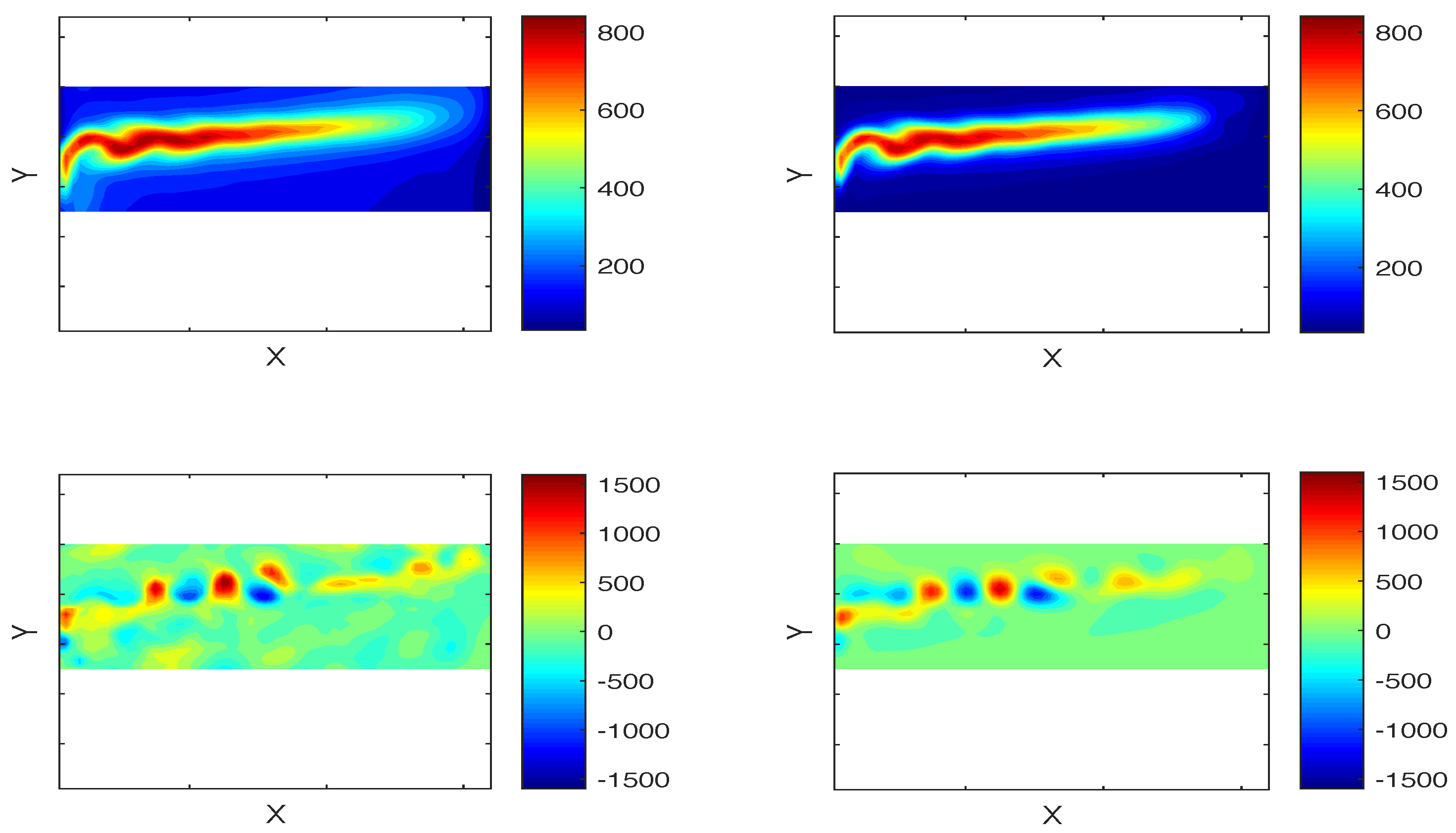
We consider a model of mid-latitude ocean gyres where flow dynamics is simulated by the three-layer quasi-geostrophic (QG) equations forced by the wind stress in the upper layer, in which merging western boundary currents form powerful eastward jet extension, similar to the Gulf Stream and Kuroshio; see Section 4.1. The ocean circulation of eddy-resolving simulation with ≈ spatial degrees of freedom (d.o.f.) at reference model parameters [8] is characterized by a robust large-scale decadal low-frequency variability (LFV) at ≈17 years and involving coherent meridional shifts of the eastward jet extension separating the gyres. This LFV is driven by transient mesoscale eddies, qualitatively similar to the turbulent oscillator studied by [60,61]; see [62,63,64,65,66,67,68] for alternative theories. Still, there is no clear scale separation between the eddies and large-scale flow, and in fact, the LFV accounts for a relatively small fraction of the total variability, as demonstrated below in the detailed DAH analysis.
First, we consider the upper-ocean stream function anomalies, given by the dataset of days, sampled 10 days apart and coarse-grained in the spatial region centered around the eastward jet (see Figure 1) with 64 points in the x-direction and 26 points in the y-direction. Then, the resulting field having time snapshots and sampled 20 days apart is compressed by applying a standard PCA [21]. The leading empirical orthogonal function (EOF) modes (from a total of 1664 modes), which capture ≈ of the total variance, are retained for the subsequent analysis. Discarded residual variability accounts for small spatial scales away from the jet; the latter being shown in Figure 1. The corresponding time series of principal components (PCs) are obtained by projecting the upper-ocean stream function anomalies onto the retained EOFs.
2.2. DAHD, DAH Power Spectrum and DAHMs
Next, we apply DAHD (Section 4.2) for the spectral analysis of the dataset constituted by the 30 corresponding PCs to diagnose, in particular, the multiscale ocean variability such as simulated by the model studied here; see Section 4.1 below for a description. Section 4.2 below recalls from [55] the main mathematical ingredients needed for the computations of the DAH spectra and modes.
To compute the latter, we first compute all the combinations of two-sided cross-correlations among the PCs time series up to lag (in sampling units) and formed the grand matrix given by (12) below with and (≈17 y), allowing us thus to resolve the decadal variability. Given the temporal sampling of 20 days used here, the Nyquist interval of resolved frequencies is therefore . After computing the DAH eigenvalues () and associated eigenvectors () of the grand matrix , we re-arrange them according to the procedure described Section 4.2.1 in order to form the DAH power spectrum given in (15), over each Fourier frequency ; see (16) below.
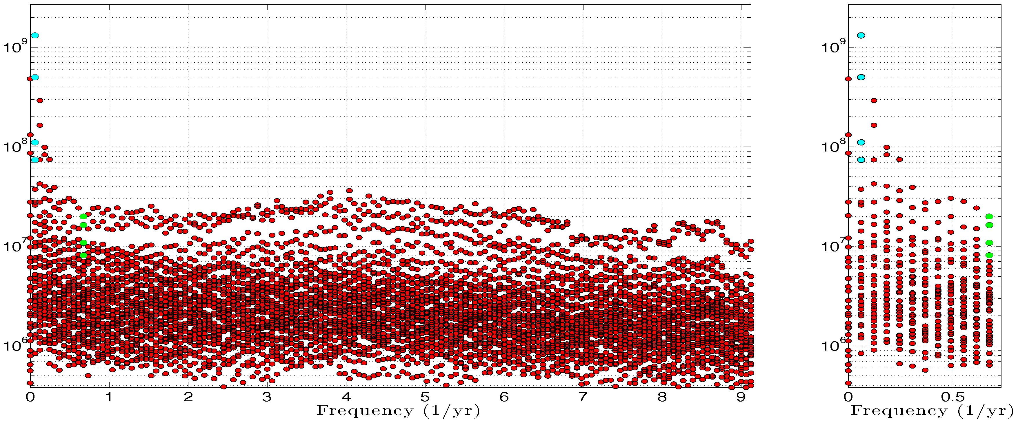
Figure 2 shows the resulting DAH power spectrum with the corresponding plotted as red filled circles. The DAH power spectrum is evenly spaced in frequency and the number of frequency bins . There are exactly pairs of at each equidistant frequency f, except at , where there are d unpaired values [55]. Note that in Figure 2 and the figures hereafter, the frequency values f that appear therein correspond to . The DAH power spectrum exhibits a complicated “bumpy” plateau-like shape stretching across most of the frequencies and without a clear distinction between fast and slow timescales; a bumpy plateau that coexists with a pronounced sharp peak at low frequencies corresponding to decadal periodicity ) as shown in Figure 2 (cyan dots in Figure 2). A closer look at the details of the DAH power spectrum indicates that the bumpy part of the plateau is actually made of much broader, but less pronounced peaks spanning over an intermediate range of frequencies, 3 < f < 6 y, as well as over a range of very high frequencies near 8.5 , thus close to the Nyquist frequency.
Recall from [55] that a separation in the DAH power spectrum between the DAH pairs at a given frequency f reflects how the singular values of the cross-spectral matrix defined by (13) are distributed. For the dataset analyzed here, while there is a large gap between dominant power values at decadal peak, other frequencies tend to have several pairs in one group that is separated above the continuous background.
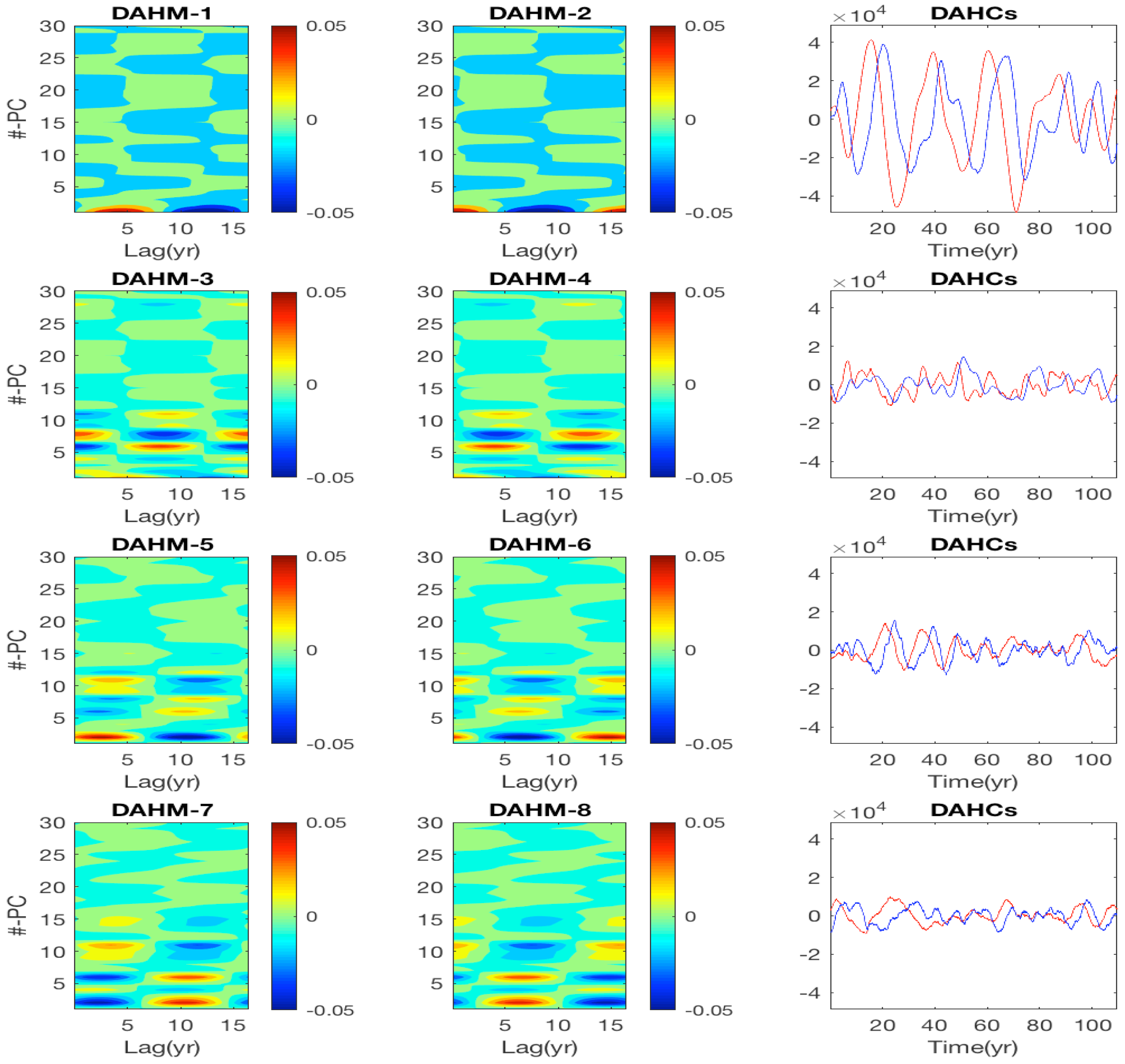
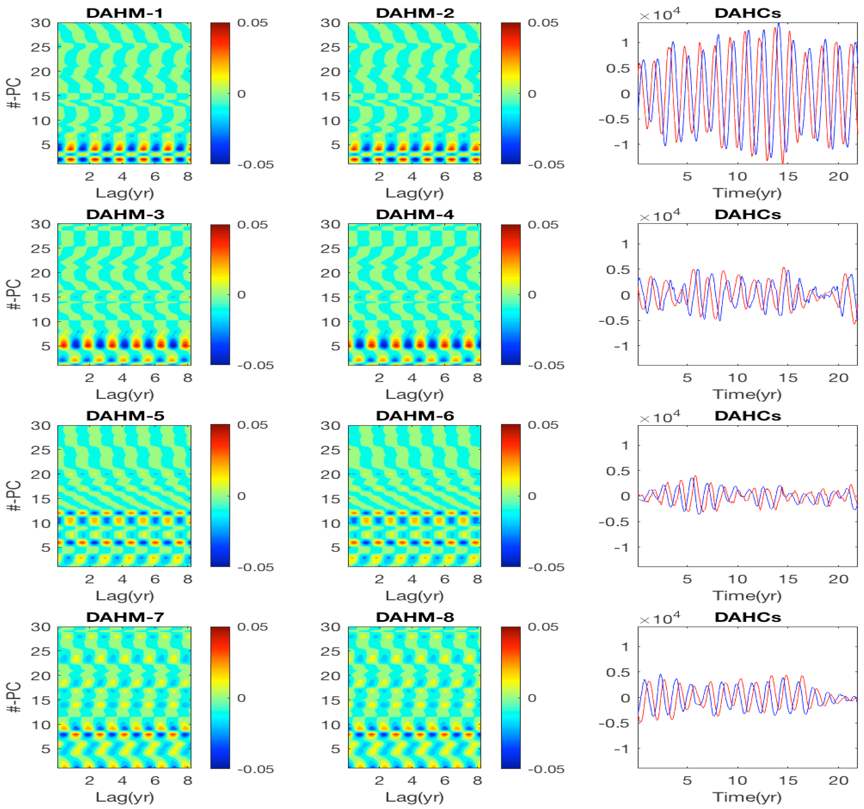
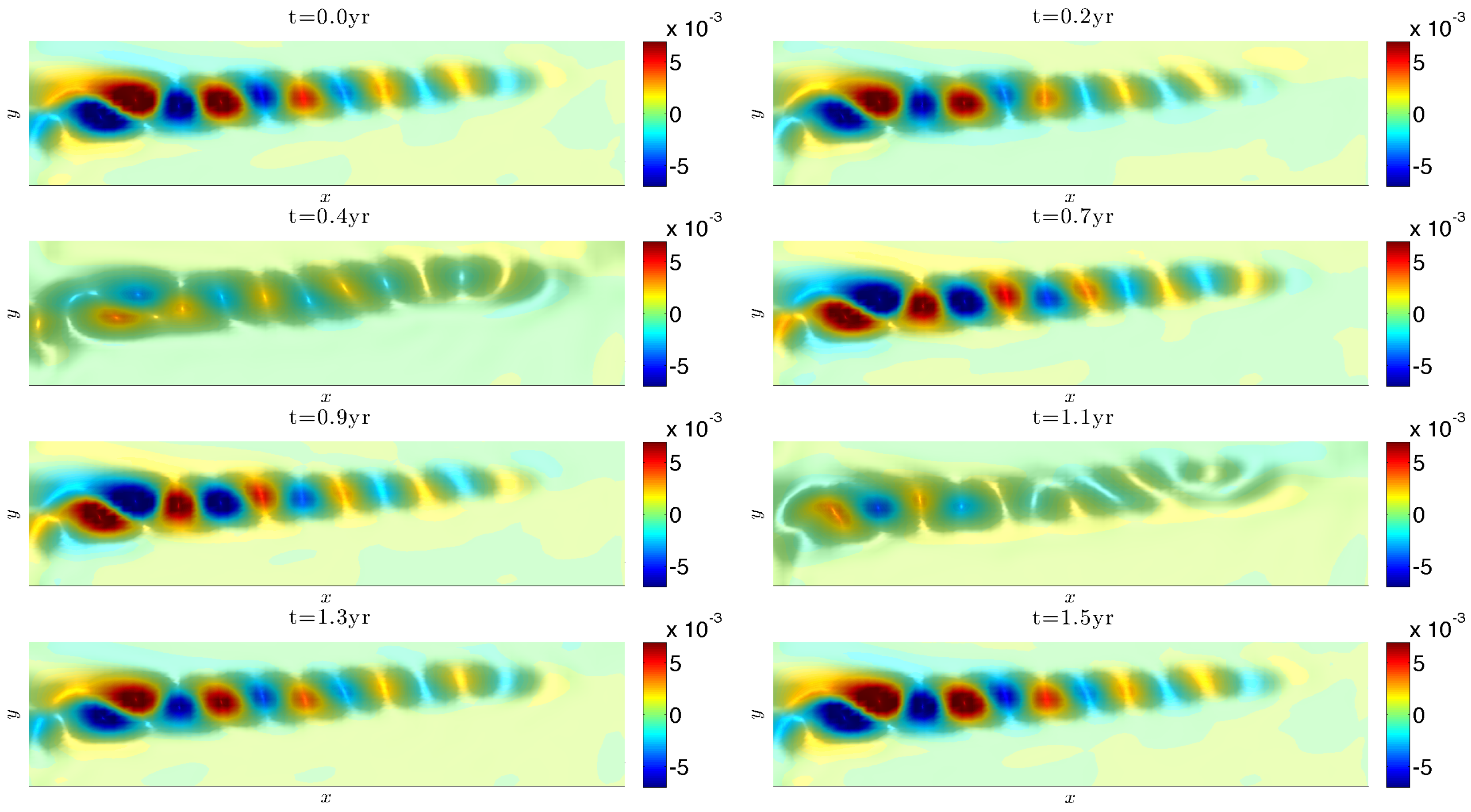
Figure 3 and Figure 4 show space-time patterns (with the “space-coordinate” taken in the EOF-phase space) for the four pairs of DAHMs (; see (17) and (18)), corresponding to the largest DAH spectral power at decadal and interannual frequency, respectively (cyan and green dots in Figure 2). The dominant modes, i.e., those corresponding to the pair having largest at these frequencies, have largest magnitude in the channels corresponding to leading PCs. As decreases, channels of higher-ranked PCs prevail with complex and non-trivial patterns. Figure 5 and Figure 6 show the oscillation phases of the dominant (associated with the largest ) DAHM patterns, when transformed back to the physical space by using EOFs. Since the DAHMs shown on the left and center columns of Figure 5 and Figure 6 have a time-component corresponding to the embedding dimension (≈17 y) [55], the transformation consists here of multiplying the 30 “spatial” channels of the DAHMs by the EOFs and then plotting in the physical space the resulting patterns as time evolves, within the embedding window. By doing so, the decadal mode reveals mostly coherent meridional shifts of the eastward jet extension, while the intraseasonal one represents largely standing oscillation of small eddies along the jet extension.
2.3. DAH-MSLM Oceanic Emulators
According to (20), the DAHCs are obtained by projection of the input dataset of retained PCs onto DAHMs and thus have = 32,500 − 299 + 1 = 32,202 data points (21). Right columns of Figure 3 and Figure 4 show that the time series of DAHCs are narrowband at the characteristic frequency associated with the respective DAHM pairs, as predicted by the theory (Section 4.2.2). Interannual DAHCs (Figure 4) appear to be very well in phase-quadrature (i.e., having a shift of a quarter of their period), since window is sufficiently long to resolve this periodicity. On the other hand, the phase-quadrature relationship is less precise for decadal DAHCs (Figure 3) since is comparable to such periodicity. Furthermore, the magnitudes of DAHCs are higher for the dominant spectral pair and tend to diminish as decreases.
To model the time-evolution of the DAHCs, we apply now the MSLM modeling approach of ([55], Section VIII) and summarized in Section 4.3 below, for the reader’s convenience. For each pair of DAHCs, the resulting MSLM model was trained to estimate coefficients for the main layer of Equations (26). The model is then integrated from initial conditions corresponding to the start of the record and is forced by a white noise realization to obtain an ensemble of simulated DAHCs. The latter are convolved with DAHMs according to (22) to obtain harmonic reconstruction components (HRCs) (23) that are added in the frequency bands of interest.
The DAH-MSLM model was estimated and run in parallel at frequencies in the full range y (see Section 4.3), taking ≈30 min of CPU time on a four-core 2.9 GHz Intel Core i7 MacBook Pro laptop to obtain a simulation of 1780 years long. On the other hand, the reference solution of the QG model (Section 4.1) takes about 1000 single-CPU hours to obtain the full data record [69].
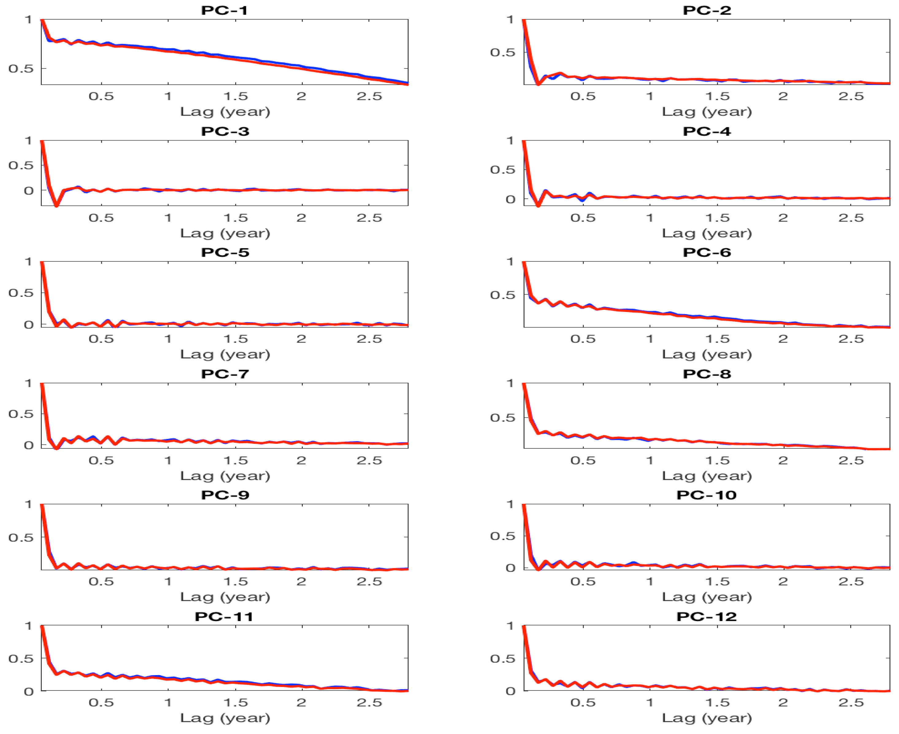
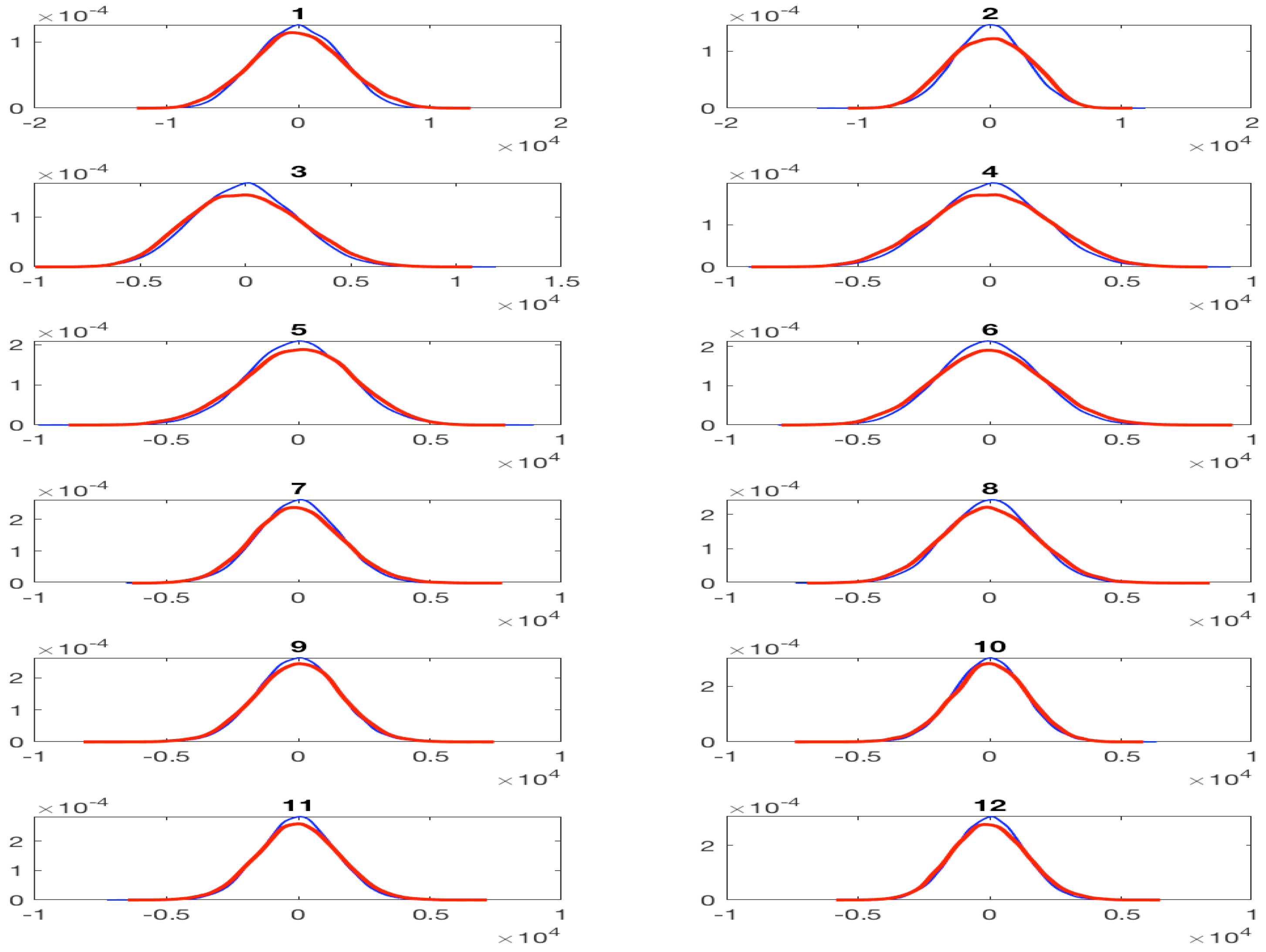
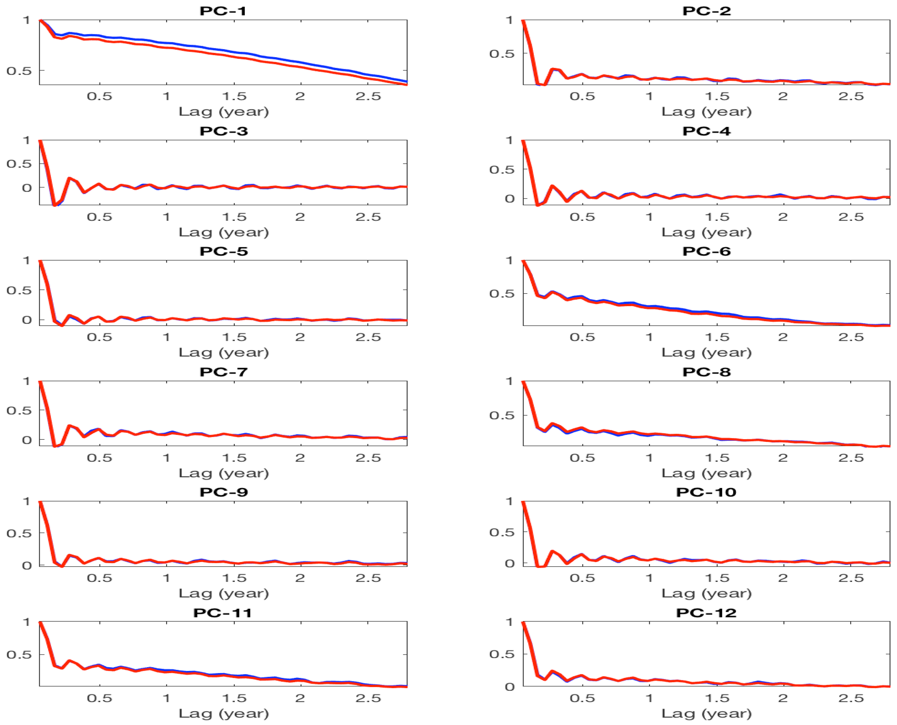
Figure A7 and Figure A8 of Appendix E below show good modeling skills of the resulting DAH-MSLM emulator in reproducing key statistical properties of leading PCs, namely their probability density functions (PDFs) and their autocorrelation function (ACFs), in a partial frequency band y. Furthermore, good statistical modeling skill is also obtained for the full range of temporal frequencies (i.e., in the Nyquist interval y), and respective results are shown in Figure A5 and Figure A6. Due in part to the long length of the simulation used here, these statistical skills do not show a marked dependence on the particular realization of the white noise used to drive our DAH-MSLM emulators. This observation is actually consistent with the ergodic property that an MSLM of the form (26) must satisfy; a property that will be communicated elsewhere. Note that for an optimal simulation of the high-frequency band 5.3 y y, it was beneficial to have and set to zero in (26).
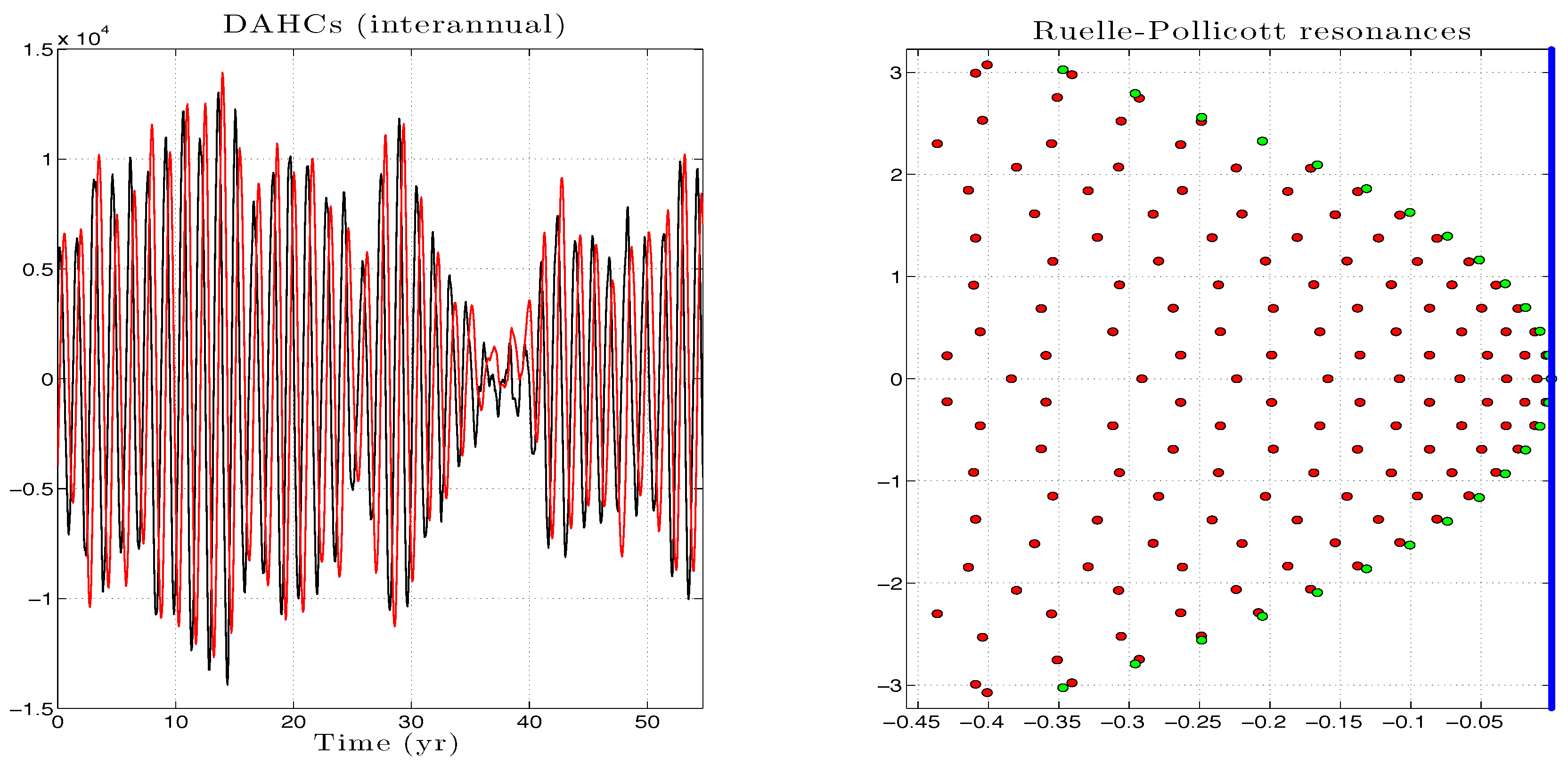
While the PDFs are mostly Gaussian, the autocorrelation functions exhibit a complicated mixture of temporal scales and thus do not allow for a clear ranking between the different PCs in terms of variability. For example, a slower decay is dominant in ACFs of PC1, 6, 8 and 11, while other PCs exhibit fast decay with superimposed oscillations. This is where a key advantage of the DAH-MSLM approach lies, i.e., in its ability to distinguish distinct temporal scales from a mixture of frequencies embedded in the data allowing in turn for an effective modeling; the distinction being under the monitoring of the DAHD, while the modeling itself is made efficient by the use of MSLMs. PC1 is shown as the black curve in Panel (a) of Figure 7. There, one can observe already in this raw time series the mixture of frequencies superimposed on a modulated oscillation of decadal dominant period. PC1 as obtained from the DAH-MSLM emulator is also shown as the black curve in Panel (b) of Figure 7.
A comparison between these two curves with the naked eye shows already that the main dominant period, as well as the time series modulations and the higher frequency part of the signal are well reproduced. To better assess how the LFV associated with the decadal oscillation is captured, we proceeded in two steps. First, for each PC1, as simulated from the QG model and from the DAH-MSLM emulator, we calculated the first four HRCs that we sum up to span a range of frequencies corresponding to the decadal variability of the flow as identified by the DAH power spectrum. The latter sum of HRCs is shown as the red and light blue curves in Panels (a) and (b) for PC1 as simulated by the QG model and the DAH-MSLM emulator, respectively. In both cases, these curves provide a low-pass filter, smoothed version, of the signal (here PC1) corresponding to the decadal variability of the flow.
In a second step, we estimated the reduced Ruelle–Pollicott resonances (Appendix A and Appendix B) associated with the reduced phase space V constituted by these sums of HRCs and their lagged versions; the lag being taken here to be equal to 1 y. Essentially, these resonances are obtained from the spectrum of the transition matrix associated with these sums of HRCs in the reduced phase space V; see Appendix B for more details. As outlined in Appendix A and Appendix B (see also Appendix C), these resonances are characteristic of the underlying dynamics, and the arrangement of these resonances in the complex plane constitutes a signature of key dynamical features. In particular, they allow for precise decomposition formulas of correlation functions and power spectral densities (PSDs) in term of these resonances; see (A5) and (A6) in Appendix A below. See also [56,70,71] and the references therein. In this sense, their estimation goes beyond the estimation of ACFs and PSDs: the latter statistical quantities could indeed share similar features without sharing necessarily the same underlying resonances. In terms of modeling, an agreement of these resonances is thus more demanding, but also more indicative of a good capture of the dynamics than by looking simply at the reproduction of ACFs and PSDs.
Panel (c) of Figure 7 shows a good agreement of the arrangements of the resulting reduced RP resonances estimated from the HRCs calculated from the QG simulations, on the one hand, and from the DAH-MSLM emulator, on the other. Such good modeling skills as diagnosed by (reduced) RP resonances are not only the attribute of the decadal variability, they are actually observed across other frequency ranges such as corresponding to interannual variability and even subannual and for most of the PCs (not shown). These results obtained in the EOF-phase space or its reduction indicate that a good agreement is expected to take place in the physical space, as well, between the simulations of the DAH-MSLM emulator and the original QG model from which it is derived.
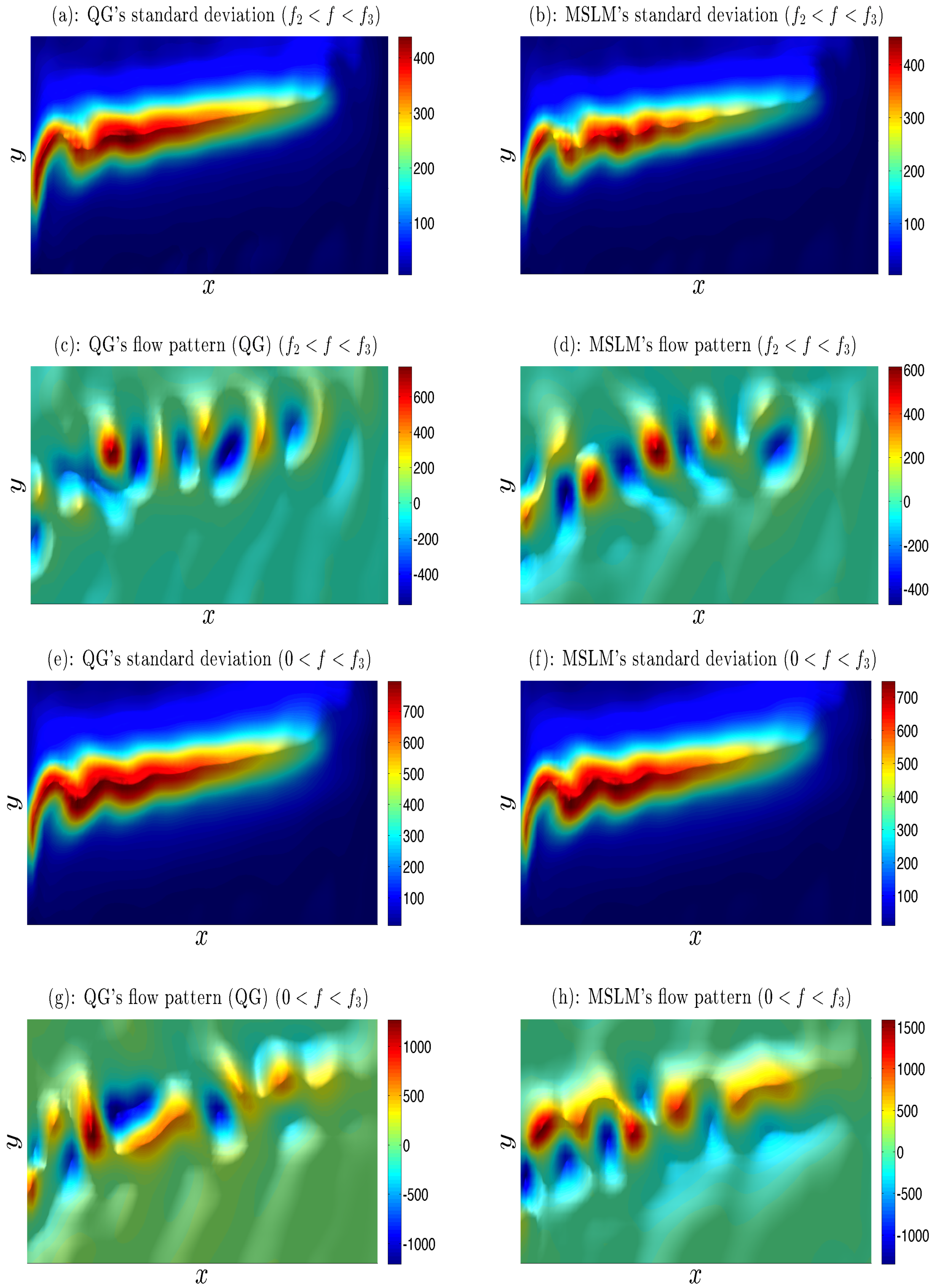
To assess the modeling skills in the physical space, the DAH-MSLM simulations (in selected frequency bands) are transformed into the physical space by using EOFs. Comparison with harmonic reconstructions of QG data in low, intermediate, high and full frequency bands shows realistic instantaneous flow patterns obtained by the DAH-MSLM emulator (compare Panel (c) (resp. (g)) with Panel (d) (resp. (h)) of Figure 8 and Figure 9), albeit this similarity is necessarily qualitative due to the stochastic nature of the latter.
In addition, the DAH-MSLM emulator reproduces very well both the spatial patterns and magnitude of variance in these key frequency bands; compare Panel (a) (resp. (e)) with Panel (b) (resp. (f)) of Figure 8 and Figure 9. Despite the pronounced decadal peak, the LFV range y accounts only for of the total variance in the full range of resolved frequencies y (in the truncated subspace of 30 leading EOFs), while most of the variance is captured by the intermediate range of temporal scales.
3. Discussion
Thus, the DAHD of the QG model’s stream function anomalies, after projection onto the space of EOFs, allows for the efficient modeling of the main statistical features of the flow and its variability across a broad range of frequencies, by a network of stochastic oscillators, namely the MSLMs. In mathematical terms, if one denotes by the anomalies of the upper-layer stream function, the DAHD provides the following representation:
where denotes the k-th EOF and the harmonic reconstructed component, at the frequency f for this EOF; see (23) in Section 4.2.2 below. Since the are themselves linear combinations of the DAHC pairs at the same frequency (see (22)), the modeling of boils down to the modeling of these pairs, due to (1). As shown above and further discussed from a theoretical viewpoint in Appendix B, Appendix C and Appendix D below, the efficient modeling of these DAHC pairs by MLSMs offers thus an interesting representation/modeling of a turbulent stream function in terms of stochastic oscillators. In a certain sense, the original quasiperiodic Landau view of turbulence [72,73], with the amendment of the inclusion of stochasticity, may be well suited to describe turbulence.
Unlike the data-driven emulator of [69], where the time-lagged multivariate singular spectrum analysis (M-SSA) basis and linear stochastic MSM formulation [54] are used to extract and simulate decadal LFV only, the DAH-MSLM approach allows us to capture the full spectrum of temporal scales, from decadal to mesoscale eddies. The key and unique features that make it possible and that are not available in other data-adaptive decompositions including M-SSA are the rigorous extraction of the spatio-temporal modes (i.e., DAHMs) unambiguously associated with a single temporal frequency (i.e., without mixing of scales) and a well-defined dynamical mechanism to describe their time evolution (i.e., respective DAHCs) using coupled Stuart–Landau stochastic oscillators. Both DAH power and phase spectra hold great promise for the dynamical diagnostics and intercomparison of multiscale datasets and models, focusing on specific frequency bands.
The future research directions include utilizing DAH-MSLM emulators for dynamical analyses, material transport and eddy parameterizations. For example, [5,8,74] approximated actual eddy effects in non-eddy-resolving models by applying transient forcings with spatio-temporal correlations. Such forcings excite flow fluctuations that evolve dynamically and eventually become rectified by the nonlinearity into the eddy-driven large-scale flow anomalies. A major interim weakness of this approach is that it treats transient forcing in the simplest way.
The DAH-MSLM modeling offers great advantages, because not only does it provide vehicles for statistically accurate approximations of the eddy field and its eddy forcing, but also it makes the above parameterization approach much more general and versatile. Instead of applying some random stochastic noise as a replacement for the eddy effects, DAH-MSLM can provide highly constrained forcing functions with spatio-temporal correlations fitted to the actual observed statistics of the eddies. The emulated eddy forcings can be embedded in the corresponding non-eddy-resolving ocean models as data-driven replacements for the eddy effects with direct [5,6,7] and indirect [8,75] implementations of the embedding.
4. Models and Methods
4.1. Mid-Latitude Ocean Model
In this study, the data are generated from the integration of the classical eddy-resolving double-gyre ocean model of [8]. The flow dynamics is governed by the quasi-geostrophic potential-vorticity (QG PV) equations for 3 stacked isopycnal layers:
where the layer index starts from the top; is the Jacobian operator; kg·m is the upper layer density; m·s is the planetary vorticity gradient; m·s is the eddy viscosity coefficient; and s is the bottom friction parameter. The basin size is km, so that and The isopycnal layer depths are = 250, = 750 and = 3000 m. The PV anomalies and the velocity stream functions are related as:
where the stratification parameters are such that the first and second Rossby deformation radii are km and km, respectively. The flow is forced by the prescribed wind stress curl The double-gyre Ekman pumping is asymmetric in order to avoid artificial symmetrization of the gyres:
where the asymmetry parameter is the non-zonal tilt parameter is and the wind stress amplitude is N·m.
There are no-flow-through and partial-slip boundary conditions on the lateral walls, augmented by the integral mass conservation constraints. The model is solved on the uniform grid with 7.5-km nominal resolution. The solution is saved every 20 days over 1780 years; this time interval is unprecedentedly long for an eddy-resolving ocean model, but our study requires this length to obtain highly accurate statistics of the flow. Each snapshot of the solution was coarse-grained by a local running-window averaging with a 120-km width to a grid with 60-km spacing. We checked that the outcome is not sensitive to moderate variations of the running-window width.
4.2. Data-Adaptive Harmonic Decomposition
The data-adaptive harmonic decomposition (DAHD) [55] is a signal-processing technique that allows for a decomposition of the power and phase spectra via data-adaptive modes within a time-embedded phase space. Unlike other techniques exploiting time-embedding, such as M-SSA [25] or its nonlinear version [28], DAHD exploits a combination of integral operator and semigroup techniques [76] that help decompose the original signal into elementary signals that are narrowband for each separate discrete Fourier frequency, while being data-adaptive.
The mathematical details of the approach are provided in [55] within a general framework, including the case of multivariate time series issued from a mixing dynamical system, either stochastic or deterministic. Central to the approach is the spectral analysis of a class of integral operators whose kernels are built from correlation functions in a quite different way than found in principal component analysis (PCA) and its generalizations. For the sake of simplicity, we recall first from [55] how such an integral operator is constructed in the case of a one-dimensional time series . Given the two-sided autocorrelation function (ACF), (of ), estimated on the interval , such an operator takes the form:
and acts on any square-integrable function on the interval I. The parameter characterizes the embedding window, but is chosen in practice so that sufficiently decays over .
At a practical level, the discretization of the operator defined by (10) leads to Hankel matrices built from temporal correlations fundamentally different than in M-SSA and alike. For multivariate time series, the ACF, , is replaced by time-lagged cross-correlations, and operators such as given by (10) are grouped into a block operator whose discretization results into block-Hankel matrices; see (12) below and ([55], Sec. VI-D). The aforementioned DAHMs are then obtained as eigenvectors of such a block-Hankel matrix, while the corresponding eigenvalues provide a notion of energy contained into the signal that, while allowing for a reconstruction of the signal, is not equivalent to variance; see ([55], Remark V.1-(ii)). The main properties of DAH spectral elements are given below.
4.2.1. DAH Eigenelements and Power Spectrum
Given a multivariate time series formed of d “channels” sampled uniformly at a unit of time , i.e., , with , , the first step to determine the DAH spectra consists of estimating the two-sided cross-correlation coefficients between channels p and q at lag k up to a maximum lag , i.e., .
As shown in ([55], Sec. VI-D), the discretization of the operator given by (10) with leads to the following Hankel matrix :
By forming such a Hankel matrix for each in , one can assemble the following block-Hankel matrix composed by blocks of size , each given according to:
Note that because each building block, , is symmetric and because , the grand matrix is itself symmetric, and therefore, its eigenvalues are necessarily real while the eigenvectors form an orthogonal set.
Furthermore, Theorem V.1 of [55] shows that the corresponding eigenvalues of come in pairs of equal absolute values, but with the opposite sign. The eigenvalues can be grouped per Fourier frequency f () and are actually determined by the singular values of a cross-spectral matrix at each frequency. In particular, denoting by the Fourier transform at the frequency f of the cross-correlation function , we consider the following cross-spectral matrix whose entries are given by:
Then, Theorem V.1 of [55] shows that for each singular value of there exists, when , a pair of negative-positive eigenvalues of such that:
i.e., eigenvalues are associated with each Fourier frequency . The same theorem shows that d (but not paired) eigenvalues are associated with the frequency .
This property allows one to rearrange the eigenvalues into the DAH power spectrum that consists of forming, for each ℓ ranging from 1–, the discrete set:
where:
Hereafter, we use for concision, re-indexing the string to run from 1– as necessary.
Furthermore, Theorem V.1 of [55] shows that the eigenvectors of can also be grouped per Fourier frequency f by using the following representation:
where DAHM snippet is a -long row vector that is explicitly associated with a Fourier frequency f according to:
where the amplitudes and the phases are both data-dependent, for each k in . Thus, we can easily sort the eigenvectors according to a given Fourier frequency in (16), by determining the following subset of indices in :
Note that is composed of indices when and of d indices if , and therefore, ’s form a partition of the total set of indices,
4.2.2. DAH Coefficients
Another useful property concerns the pair of DAHMs associated with a pair of DAH eigenvalues , such that with j and that belong thus to the same subset . For such a DAHM pair, the theory shows indeed that their corresponding phases satisfy , i.e., in each DAHM pair, the modes are shifted by one fourth of the period; see Theorem IV.1 of [55]. The DAHMs are thus always in exact phase quadrature, as for a sine-and-cosine pair in Fourier analysis, but in a data-adaptive fashion as encapsulated in the ’s and the ’s.
By analogy with M-SSA [25], the multivariate dataset X can be projected onto the orthogonal set formed by the ’s, in order to obtain the following DAH expansion coefficients (DAHCs):
where t varies from one to:
Although the DAHCs are not formally orthogonal in time, the DAHC pair associated with a DAHM pair , is composed of time series that are nearly in phase quadrature; a property that is all the more pronounced when the embedding window parameter M can be made sufficiently large to resolve the decay of temporal correlations contained in X; see [55]. In other words, the larger M (subject to the length of the record), the more apparent is the phase quadrature property exhibited by and constituting a DAHC pair.
Furthermore, any subset of DAHCs, as well as the their full set, can be convolved with its corresponding set of DAHMs, to produce a partial or full reconstruction of the original dataset, respectively. Thus, the following j-th reconstructed component (RC) at time t and for channel k is defined as:
where (resp. ) is a lower (resp. upper) bound in , that is allowed to depend on time. The normalization factor equals , except near the ends of the time series, as in M-SSA [25], and the sum of all the RCs recovers the original time series.
Due to the ordering of the DAHMs in terms of Fourier frequency, the harmonic reconstruction component (HRC) can be formed from the sum of the RC pairs associated with a same Fourier frequency , namely:
where denotes the set of indices given in (19). HRC provides an unambiguous and natural way to determine how variability at a particular frequency f is expressed in the time domain. For instance, Panels (a) and (b) of Figure 7 show the sum of the first four HRCs on PC1 for the upper-layer stream function anomalies as simulated from the QG model and its DAH-MSLM emulator, respectively.
4.3. Multilayer Stuart–Landau Models
DAHD facilitates efficient inverse modeling of a given multivariate dataset in the transformed coordinates of DAHCs (20) and then utilizes the reconstruction Formulas (22) and (23) for transformation into the space of the original variables of . As we explain below, the modeling of DAHCs is simplified due to (i) the near-phase quadrature property satisfied by any DAHC pair and (ii) its narrowband character.
Let us consider a DAHC pair associated with a pair of DAH eigenvalues , such that with j and that belong thus to the same subset associated with a frequency f. Moreover, without loss of generality, we can assume that is positive and is negative. Hereafter, we also assume the time t to be a continuous parameter. For such a DAHC pair, we form the complex time series, where . As shown in Section VII of [55], we can infer that:
Since the convolution term in the RHS of (24) involves a cosine function oscillating at the frequency f, the frequencies contained in the time series are filtered out, and the resulting DAHC, , is narrowband about the frequency f. This latter property is shared by all DAHCs, , with j in , and in particular for . Although the RHS of (24) provides an exact representation of the DAHC (in the case of an infinite time series), its usage in practice is limited since we desire a closure model of the ’s that avoids an explicit dependence on the data, , as found in (24).
Guided by the fact that a DAHC pair is composed of narrowband time series that are nearly in phase quadrature, Chekroun and Kondrashov [55] have shown that the class of Stuart–Landau (SL) oscillators driven by an additive noise [77,78] represent a natural class of closure models to capture amplitude modulations of and :
where and are real parameters, is a noise term and . Complementarily, Appendix A, Appendix B, Appendix C and Appendix D below justify the modeling of DAHCs within the class of SL oscillators by the theory of Ruelle–Pollicott (RP) resonances and their estimation from the time series. Furthermore, the collective behavior of all DAHC pairs associated with the same frequency f must be also taken into account by using an appropriate dynamical coupling between the corresponding individual SL oscillators, as well as by considering temporal and spatial cross-pair correlations in the noise term .
The multilayer MSM framework of [54] is particularly suited to deal with these issues and applied to (25), it leads to MSLMs such as introduced in [55]. For this study, the optimal MSLM has only a main layer according to the stopping criterion described in Appendix A of [54], and it is given as the following system of SDEs driven by pairwise-correlated white noise:
Appendix C and Appendix D below provide, in the context of the data collected from the oceanic model [8], numerical evidences and theoretical arguments for the modeling of the corresponding DAHCs by MSLMs such as (26). As mentioned above, the theoretical apparatus is in particular based on the theory of Ruelle–Pollicott resonances and their estimation from time series [56], recalled in Appendix A and Appendix B below.
Here, is aimed at approximating a DAHC pair associated with a frequency , and the index j belongs to the subset of indices associated with d distinct pairs. The ’s with or , and , form independent Brownian motions.
Following Kondrashov et al. [54], all model coefficients are estimated for each -pair by (multiple) linear regression (MLR). Linear constraints on and are imposed to ensure antisymmetry for the linear part of each -pair, as well as equal and positive values to ensure asymptotic stability. The resulting regression residuals yield time series of that are well approximated by pairwise-correlated white noise in the sums involving the ’s; see Appendix D for more details. Note that an MSLM, as any MSM, may include more layers to accurately model the regression residual; see Section VIII-B of [55]. It turned out that for the simulations reported in this study, an MSLM of the form (26) was sufficient to reach satisfactory modeling skills; see Figure 8 and Figure 9 above, as well as Appendix E. Note also that the DAHCs associated with are not paired and resemble red noises in practice (see [55]); thus, only a linear MSM is used to model the DAHCs associated with the zero-frequency; see [54].
Because the SL oscillators are uncoupled across the frequencies, the DAH-MSLM approach is computationally efficient, totally parallelizable and, for a variety of datasets, laptop-enabled in practice. First, the model coefficients can be estimated in parallel for each frequency, and the overall number of independent coefficients to estimate remains small and fixed for each -pair. Once all the resulting (few) MSLM coefficients have been estimated, for the simulation, as well, no extra coupling across the frequencies is needed other than running the MSLMs across the frequencies by the same noise realization, which can be also done in parallel.
To simulate the DAHC pairs, Equations (26) are discretized in time and integrated numerically forward using a Euler–Maruyama scheme from initial states obtained according to the initialization procedure described in Appendix B of [54], followed by a convolution with the associated DAHMs according to (22) to transform into the space of original variables. The simulated RCs are then added in each frequency bin to yield the corresponding HRCs given by (23) that, in turn, are added across the frequencies in the range of interest. For instance, Panel (b) of Figure 7 shows the sum of the first four HRCs on PC1 for the upper-layer stream function anomalies as simulated for the DAH-MSLM emulator of the QG model considered here.
Acknowledgments
This research was supported by the National Science Foundation grants OCE-1243175 and OCE-1658357 (Dmitri Kondrashov and Mickaël D. Chekroun) and DMS-1616981 (Mickaël D. Chekroun). Pavel Berloff was supported by the NERC grant NE/R011567/1.
Author Contributions
Dmitri Kondrashov, Mickaël D. Chekroun and Pavel Berloff conceived of and designed the experiments. Dmitri Kondrashov and Mickaël D. Chekroun performed the experiments. Dmitri Kondrashov and Mickaël D. Chekroun analyzed the data. Dmitri Kondrashov, Mickaël D. Chekroun and Pavel Berloff wrote the paper.
Conflicts of Interest
The authors declare no conflict of interest.
Abbreviations
The following abbreviations are used in this manuscript:
| DAH | Data-adaptive harmonic |
| DAHD | Data-adaptive harmonic decomposition |
| DAHC | Data-adaptive harmonic coefficient |
| DAHM | Data-adaptive harmonic mode |
| EOF | Empirical orthogonal function |
| HRC | Harmonic reconstructed component |
| LFV | Low frequency variability |
| MSLM | Multilayer Stuart–Landau model |
| PCA | Principal component analysis |
| PSD | Power spectral density |
| RC | Reconstructed component |
| RP | Ruelle–Pollicott |
| SDE | Stochastic differential equation |
| SL | Stuart–Landau |
Appendix A. Time Variability of Stochastic Systems and Ruelle–Pollicott Resonances
We communicate in this Appendix and the subsequent ones the mathematical foundations for the modeling of DAHCs by the class of Stuart–Landau models (25) and their generalization given by (26). The theoretical apparatus is based on the theory of Ruelle–Pollicott (RP) resonances and their numerical estimation from time series, following [56]. We recall below the main ingredients of this theory, in particular regarding the fundamental role that RP resonances play in the decomposition of power spectral density (PSD) and correlation functions and that we apply to the case of time series constituted by the dominant pairs of DAHCs for the three frequency bands of interest in this study, namely decadal, interannual and subannual.
Given a system of stochastic differential equations (SDEs) in ,
Here, denotes an -valued Wiener process whose components are mutually independent standard Brownian motions.
In Equation (A1), the drift part is provided by a (possibly nonlinear) vector field F of , and the (also possibly nonlinear) stochastic diffusion in its Itô version, given by , has its i-th-component () given by:
In what follows, we assume that the vector field F and the matrix-valued function:
satisfy regularity conditions that guarantee the existence and the uniqueness of mild solutions, as well as the continuity of the trajectories; see, e.g., [79,80] for such conditions in the case of locally Lipschitz coefficients.
It is well known that the evolution of the probability density of the random -valued variable, (solving Equation (A1)), is governed by the Fokker–Planck equation:
with .
What is less-known however is that the spectral properties of the second-order differential operator, , informs about fundamental objects such as the power spectra or correlation functions computed typically along a (random) trajectory of Equation (A1). We briefly recall the main elements hereafter and refer to [56,71] for more details.
First, given an observable for the system (A1), we recall that the correlation spectrum is obtained by taking the Fourier transform of the correlation function , namely:
where denotes the stochastic process solving (A1) and satisfying at time .
As shown in [71], for a broad class of SDEs that possess an ergodic probability distribution , the spectrum, , of the Fokker–Planck operator, , is typically contained in the left-half complex plane, , and its resolvent , is a well-defined linear operator that satisfies:
Here, f lies in the complex plane , and the poles of the resolvent , which correspond to the RP resonances, introduce singularities into . Once the PSD is calculated, i.e., once is computed with f taken to be real, these poles manifest themselves as peaks that stand out over a continuous background at the frequency f if the corresponding RP resonances with imaginary part f (or nearby) are close enough to the imaginary axis. The continuous background has its origin in the continuous part of lying typically in a sector (for some ), while the RP resonances are the isolated eigenvalues of finite multiplicity of , lying within a strip ; see Panel (A) of Figure A1.
Denoting by ’s the poles of the resolvent of , i.e., the Ruelle–Pollicott resonances, and by their corresponding orders, the correlation function, , possesses then the following expansion:
where exhibits typically a decay property associated with properties of the essential spectrum of . Note that even if the ’s do not depend on the observable , the coefficients, ’s, in the expansion (A6), do.
Historically, the resonances have been introduced by Ruelle [81] and Pollicott [82] for discrete and continuous chaotic deterministic systems (see [83] for the case of Anosov flows), but can be framed easily into a stochastic context, which benefits then from the tools of stochastic analysis, which allows, e.g., for justifying decomposition formula such as (A6) for a broad class of SDEs; see [70,71,84].
Figure A1.
(a) The Ruelle–Pollicott (RP) resonances are the isolated eigenvalues of the Fokker–Planck operator, , defined in (A3); they are represented by red dots in (b) and by black dots here. The rightmost vertical line represents the imaginary axis above which the power spectrum lies; see (a) for another perspective. The rate of decay of correlations is controlled by the spectral gap (not to be confused with in (A6)); see [56,85]. (b) The imaginary part of the RP resonances corresponds to the location of a peak in the PSD (black curve lying above the imaginary axis) and the real part to its width. In blue is represented a reconstruction of the PSD based on RPs; a discrepancy is shown here to emphasize that in practice, the RPs are very often only estimated/approximated; see [56,71] (courtesy of Maciej Zworski). (a) Schematic of the spectrum of given in (A3). (b) Correspondence between the PSD and RP resonances according to (A5).

Appendix B. Estimating Resonances from Time Series: The Reduced RP Resonances
Because they are related to the Fokker–Planck operator, , the RP resonances inform about the structure of the underlying SDE. A natural question then arises: is it possible to infer the “shape” of an SDE (i.e., F and G in (A1)) from the observation of its solutions? The short answer to this question is “no” in general, except in certain cases (see [86]), but as we will see, a reduced spectrum, related to RP resonances, can be estimated from time series and depending on its geometry may inform us greatly in turn about the sought structural ingredients. In that respect, the approach of [56] paved a roadmap for addressing this question from a practical viewpoint; we refer to [71] for theoretical foundations.
In practice, only partial observations of the solutions to (A1) are available, e.g., few solution components. Speaking roughly, it is shown in [56] that given partial observations of a complex system that lie in a reduced phase space V, a Markov operator with state space V can be inferred from these observations such that (i) characterizes the coarse-graining in V of the transition probabilities in the full state space and (ii) the spectrum of relates to the RP resonances, but in an averaged sense; see also [29,87]. In practice, the dimension of V is kept low so that can be efficiently estimated via a maximum likelihood estimator (MLE). We detail below this procedure and what (ii) means, in the context of DAHCs.
Our standing assumption is that for each frequency , there exists a model of the form (A1) of which a solution is given by the set of DAHC-pairs, , at frequency f. Under this working assumption, since there is a total of d pairs, our phase space is here with . Our observations are made out of a single pair of DAHCs, , so that dim(V) = 2 here. We denote by the corresponding mapping and take , i.e., discrete time instants, as given by the multiple of the sampling time at which the DAHCs are computed, here 20 days.
The Markov operator is approximated by the transition matrix P whose entries are given:
where the ’s form a partition (of size ) of a domain in containing the set of discrete points , for ; see, e.g., [56,87,88].
Assuming that the sought system of SDEs, (A1), possesses an ergodic statistical equilibrium, , one can show that in the limit , the spectrum of P (after application of the (principal value of) logarithm) provides an approximation of the point spectrum of the following averaged Fokker–Planck operator, given formally for all in by:
see [89]. The point spectrum of provides what we call hereafter the reduced RP resonances of . In [71], it is called the reduced mixing spectrum, terminology that we have purposely changed here to avoid any confusion with the notion of mixing in the physical space; the mixing referred to in [71] takes place in the phase space and is typically manifested by decay of correlations; see also [56]. The point spectrum characterizes the mixing properties in the reduced phase space, once the effects of the variables lying in the unobserved factor Z have been averaged out. Thus, in short,
More precisely, in (A8), the space Z denotes the supplement of V in , i.e., , and denotes the disintegration of above v in V, along the unobserved factor space Z. Mathematically, for all Borel sets B and F of Z and V, respectively,
with ; see [54] and the references therein. Thus, the operator corresponds to the conditional expectation of obtained after averaging along the unobserved variables lying in Z. Once the Markov matrix P is estimated from time series via (A7), its spectrum provides in turn an estimation of the reduced RP resonances and thus may inform us about the nature of the coefficients of provided that the spectrum of P exhibits interpretable features in terms of known SDEs.
To illustrate this point, we focus first on the dominant pair of DAHCs for the interannual frequency, namely . The time series constituting this pair of DAHCs are shown in the left panel of Figure A2. The corresponding transition matrix P is estimated by using (A7) for this pair of DAHCs and the state space over which this matrix is estimated and taken to be with:
and:
for some . Here, N = 32,200, and a (non-uniform) partition of constituted by cells ’s is considered.
The spectrum of P thus estimated is shown in the right panel of Figure A2 (in red), after application of the logarithm. It is striking to observe that the corresponding eigenvalues are organized into an array of shifted parabolas, at least for most of these eigenvalues. This special geometry reflects actually key structural properties about the averaged Fokker–Planck operator as we explain hereafter.
Figure A2.
Reduced RP resonances and their analytic approximation. Left panel: The pair of DAHCs analyzed. Right panel: Corresponding eigenvalues of P as estimated by using (A7), after application of the logarithm (in red). The blue vertical line corresponds to the imaginary axis. These eigenvalues correspond to approximations of the point spectrum of the averaged Fokker–Planck operator given in (A8). The analytic approximations provided by (A17) are shown as green dots.
Appendix C. RP Resonances of Stuart–Landau Models: Analytic Approximations
Let us consider the following special case of a Stuart–Landau model Equation (25) given in Cartesian coordinates by:
In polar coordinates with and , this system becomes by applying the Itô’s formula:
where and are two Wiener processes satisfying the relationships
The Fokker–Planck equation associated with (A14) is given by:
We assume now that is sufficiently largely positive and is sufficiently small, so that roughly speaking, the dynamics of settles near a circle of radius , corresponding to an average radius of the stochastic limit cycle [90]. Under this assumption, it is expected thus that the azimuthal component of the solutions of (A15) can be well approximated by the solutions of the following advection-diffusion equation with periodic boundary conditions:
The solutions of (A16) are formally given by:
It is then easy to obtain the following approximation formula (up to a rescaling) for the eigenvalues, , of the Fokker–Planck operator’s azimuthal part associated with Equation (A15):
We refer to [89] for more details; see also [91]. Note that here, T in (A17) denotes the period associated with the azimuthal velocity such that .
The analytic approximations given by (A17) are shown by the green dots in the right panel of Figure A2 for and days. To such analytic approximation of the RP resonances associated with (A13), the parabolas of resonances that are shifted to the left of the complex plane by , namely:
constitute parabolas of harmonics; see [71]. These parabolas of harmonics, shown in green here for one of them to avoid overload, provide good approximations of most of the resonances shown (in red) in the right panel of Figure A2.
Note that in practice, the shift relates to the eigenvalues of the radial part of the Fokker–Planck operator associated with (A15), namely:
In particular, the smallest can be measured from the estimated resonances and informs on the value of ( by assumption) via the formula:
while the other constants appearing in (A18) are given by with k in ; see again [71] and also [92].
Thus, the numerical estimation of the eigenvalues of the transition matrix P for the pair of DAHCs associated with the interannual frequency, , combined with the analytic description outlined above reveal that the Fokker–Planck operator associated with an SL model of the form (A13) constitutes a very good approximation of the (abstract) averaged Fokker–Planck operator given by (A8). Such a spectral analysis strongly supports the idea of modeling DAHCs within the class of SL models, at least for the interannual variability of the flow. The next section of this Appendix discusses briefly the case of other frequency bands. As emphasized below, although more ingredients may be required for their good modeling, SL models still form a natural class for a coherent modeling of the subset of DAHC pairs associated with a given frequency .
Appendix D. Multilayer Stuart–Landau Modeling of DAHCs
After the material and numerical results presented in Appendix A, Appendix B and Appendix C above, we are in a position to explain the motivations behind the form (26) of MSLMs given in the main text. To understand these motivations, we formalize a bit more the writing of (26) by introducing the notations to denote a DAHC pair and to denote a two-dimensional Brownian motion.
Let us introduce the n-dimensional variable such that , and with . Then, (A21) can be re-written itself as:
Here, is a block-diagonal matrix, where each non-zero block is given by the ’s, is the n-dimensional vector formed by the collection of two-dimensional vectors written in the -variable and (resp. ) is the matrix whose blocks are given by the ’s (resp. ’s).
In practice, it is under the form (A24) that the coefficients are estimated from the time series of (all) the DAHC pairs associated with a common frequency f. This estimation is made in two steps: first, the coefficients in L, F and C (respecting the constraints on L and F) are estimated via, e.g., regression techniques, from which the -dimensional time series of residual is stored. By computing the covariance matrix of , the grand matrix is then obtained via the Cholesky decomposition of , namely .
The coupling terms are of two types: those brought by the matrix and those brought by the noise matrix . In the absence of these coupling terms, we are just left with a collection of uncoupled SL models of the form (A13). Even for frequencies f (such as in Appendix B) for which individual SL models provide very plausible SDE generators of any given pair of DAHCs at the frequency f (such as explained in Appendix C), it is unlikely to obtain in this simplified fashion a coherent simulation of the DAHCs (associated with frequency f) that would share phase relationships consistent with those exhibited by the original DAHCs (at the same frequency). It is one of the main motivations for the presence of such coupling terms in (A21) and thus in (A24).
In the presence of coupling terms, it is noteworthy that the averaged Fokker–Planck operator associated with (A24) differs from that associated with an individual SL model, i.e., associated with:
by first-order and second-order partial differential operators involving averaging over a combination of coefficients in and , respectively.
The analysis conducted in Appendix C suggests thus that any “deviation” from parabolas of the arrangement of resonances could serve as a good indication that the presence of such derivatives in the averaged Fokker–Planck operator is non-negligible (emphasizing thus the presence of coupling terms), although such a statement should be taken with care due not only to possible estimation errors that could lie behind such discrepancies, but also to other factors governed e.g., by the ratio between and , adopting the notations of Appendix C; see [89] for more details.
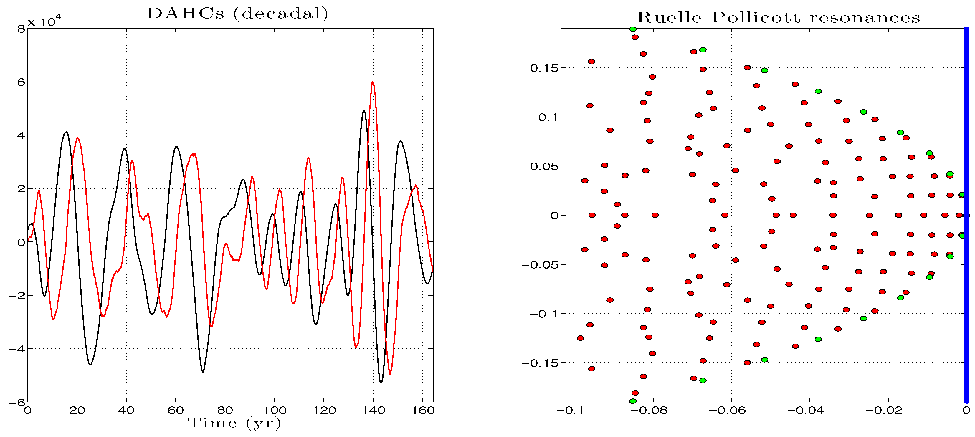
Discrepancies with respect to an array of parabolas are observed in the right panel of Figure A3 for the RP resonances estimated from the dominant pair of DAHCs shown in the left panel of Figure A3, for the frequency cycle/, i.e., corresponding to decadal variability (). The reason here lies presumably in the less precise phase-quadrature relationship thatthe time series composing such a pair satisfies, as pointed out already in Section 2.3 for the pairs of DAHCs shown in Figure 3 associated with decadal variability. Actually, not only the phase-quadrature relationship among the time series constituting a DAHC pair is altered at low-frequency, but also their narrowband character unlike for the interannual and subannual cases (not shown). This alteration of such narrowband features is actually rooted into windowing effects since the 16.4--period is actually pretty close to the size of the window (≈17 y) used to estimate the correlations underlying the DAH grand matrix, , in (12).
Thus, we may naturally expect that a single SL model (for which in particular such phase-quadratures are typically observed) is insufficient for modeling purposes. Nevertheless, the outer envelope of these resonances still follows closely a parabola as shown by the green dots in Figure A3 obtained by application of the analytic Formula (A18) with y, and The coupling terms in (A24) and the noise matrix are aimed at modeling the differences from an array of parabolas within the envelop’s convex hull.
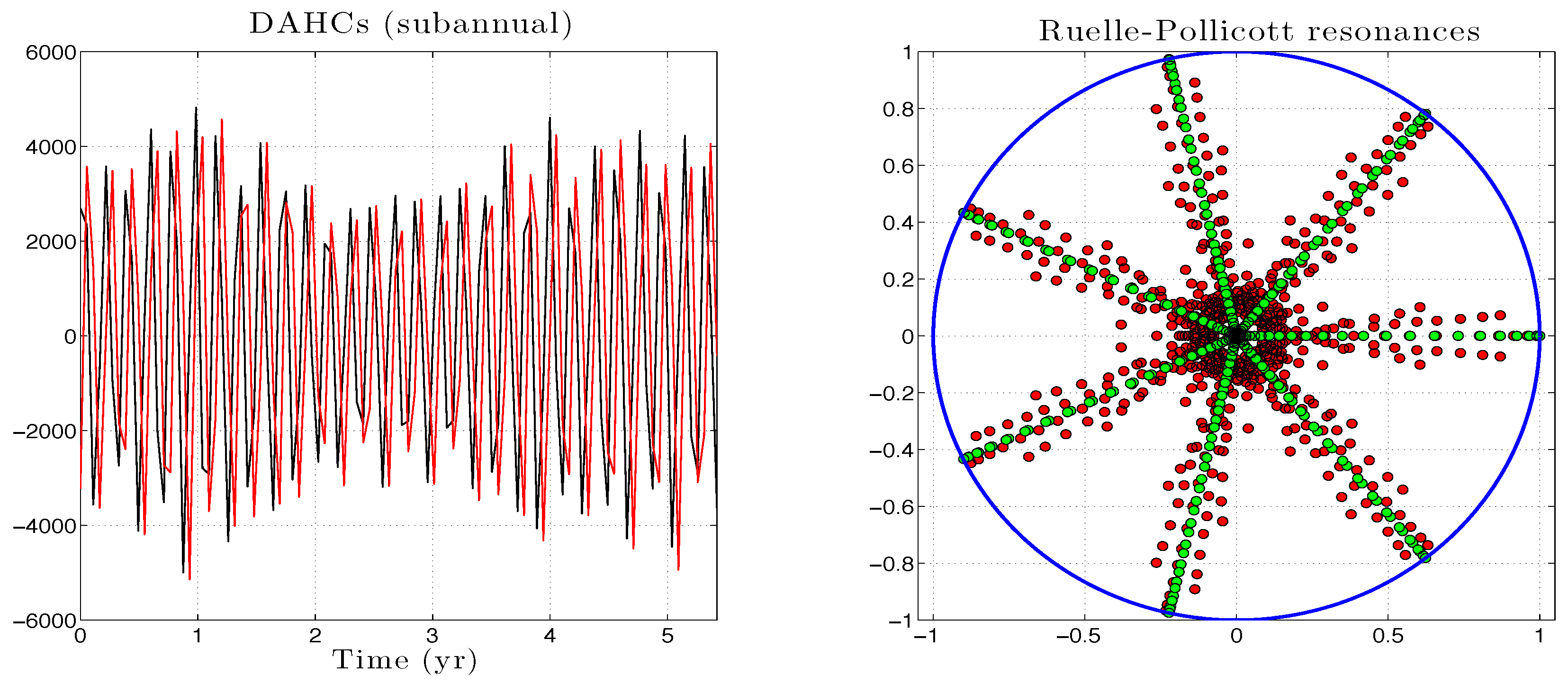
The subannual case supports also the relevance of the analytic prediction (A17) and thus of the class of Stuart–Landau models used to model the DAHCs for the corresponding frequencies, albeit in a less direct way. Here, the frequency associated with the pair of DAHCs analyzed hereafter is determined via the DAH spectrum given in Figure 2. The corresponding value of this frequency is cycle/. It lies close to the Nyquist frequency, and therefore, sampling effects are expected to manifest. For instance, whereas the dominant period should be thus as predicted by the theory, an estimation of the resonances as eigenvalues of the Markov matrix P with entries given by (A7) shows an estimated period of y corresponding approximately to . The latter period is clearly visible by displaying the eigenvalues of P without applying the logarithm, unlike in Figure A2 and Figure A3: seven strings of resonances are indeed apparent in the right panel of Figure A4 within the unit disc of the complex plane, i.e., by adopting the same mode of representation as in [56]. These resonances strings are very well approximated by rays of resonances obtained by application of the analytic Formula (A17), this time with (and not with ), and ; see the right panel of Figure A4. Note that a cluster of resonances has formed near the center, this cluster corresponding to an approximation of the essential spectrum of the Markov operator (see Appendix B) that P approximates; see [56].
In summary, the theory of Ruelle–Pollicott resonances and their estimation via time series [56] provide strong theoretical elements for the numerical modeling of DAHCs build up on MSLMs such as given by (26); see Section VIII of [55] for a generalization of (26). Note that the discussion conducted above about the subannual and decadal cases emphasizes that for practical purposes, it is not necessarily a good idea (for the estimation stage of an MSLM’s coefficients) to constrain the coefficients in (A22) to be given by , due to sampling or windowing effects such as manifested here for the subannual and decadal cases, respectively.
Figure A3.
Reduced RP resonances and their analytic approximation. Same as in Figure A2, but for the frequency cycle/.
Figure A3.
Reduced RP resonances and their analytic approximation. Same as in Figure A2, but for the frequency cycle/.

Figure A4.
Reduced RP resonances and their analytic approximation. Same as in Figure A2, but for the frequency cycle/.
Figure A4.
Reduced RP resonances and their analytic approximation. Same as in Figure A2, but for the frequency cycle/.

Appendix E. Modeling Skills in the EOF Space
In this section, we communicate on the modeling skills in the space of EOFs. These skills are assessed by comparing the probability density functions (PDFs) of the twelve leading PCs of upper-layer stream function anomalies in Figure A5 and Figure A7, as well as their autocorrelation functions (ACFs); see Figure A6 and Figure A8.
Figure A5.
Same format as in Figure A7, but the comparison of harmonic reconstruction (red) and DAH-MSLM stochastic simulation (blue) in a full frequency band .
Figure A5.
Same format as in Figure A7, but the comparison of harmonic reconstruction (red) and DAH-MSLM stochastic simulation (blue) in a full frequency band .
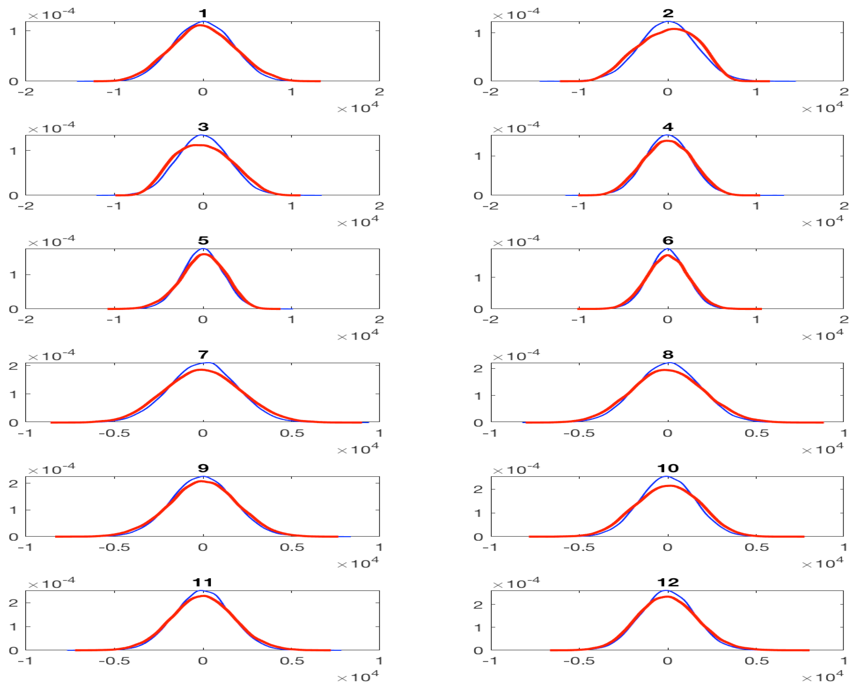
Figure A6.
Same format as in Figure A8, but the comparison of harmonic reconstruction (red) and DAH-MSLM stochastic simulation (blue) in a full frequency band .
Figure A6.
Same format as in Figure A8, but the comparison of harmonic reconstruction (red) and DAH-MSLM stochastic simulation (blue) in a full frequency band .

Figure A7.
Probability density function (PDF) of the twelve leading PCs of upper-layer stream function anomalies, DAH-filtered in a frequency band : Red, harmonic reconstruction of QG data (HRC; cf. (23)); blue, DAH-MSLM stochastic simulation.
Figure A7.
Probability density function (PDF) of the twelve leading PCs of upper-layer stream function anomalies, DAH-filtered in a frequency band : Red, harmonic reconstruction of QG data (HRC; cf. (23)); blue, DAH-MSLM stochastic simulation.

Figure A8.
Autocorrelation function (ACF) of the twelve leading PCs of upper-layer stream function anomalies, DAH-filtered in a frequency band : Red, harmonic reconstruction of QG data (HRC; cf. (23)); blue, DAH-MSLM stochastic simulation.
Figure A8.
Autocorrelation function (ACF) of the twelve leading PCs of upper-layer stream function anomalies, DAH-filtered in a frequency band : Red, harmonic reconstruction of QG data (HRC; cf. (23)); blue, DAH-MSLM stochastic simulation.
References
- Gent, P.; McWilliams, J. Isopycnal mixing in ocean circulation models. J. Phys. Oceanogr. 1990, 20, 150–155. [Google Scholar] [CrossRef]
- Eden, C. A closure for meso-scale eddy fluxes based on linear instability theory. Ocean Model. 2011, 39, 362–369. [Google Scholar] [CrossRef]
- Leith, C.E. Stochastic backscatter in a subgrid-scale model: Plane shear mixing layer. Phys. Fluids A Fluid Dyn. 1990, 2, 297–299. [Google Scholar] [CrossRef]
- Berloff, P.S.; McWilliams, J.C. Material transport in oceanic gyres. Part III: Randomized stochastic models. J. Phys. Oceanogr. 2003, 33, 1416–1445. [Google Scholar] [CrossRef]
- Berloff, P.S. Random-forcing model of the mesoscale oceanic eddies. J. Fluid Mech. 2005, 529, 71–95. [Google Scholar] [CrossRef]
- Porta Mana, P.; Zanna, L. Toward a stochastic parameterization of ocean mesoscale eddies. Ocean Model. 2014, 79, 1–20. [Google Scholar] [CrossRef]
- Jansen, M.; Held, I. Parameterizing subgrid-scale eddy effects using energetically consistent backscatter. Ocean Model. 2014, 80, 36–48. [Google Scholar] [CrossRef]
- Berloff, P. Dynamically consistent parameterization of mesoscale eddies. Part I: Simple model. Ocean Model. 2015, 87, 1–19. [Google Scholar] [CrossRef]
- Chorin, A.J.; Hald, O.H.; Kupferman, R. Optimal prediction with memory. Physica D 2002, 166, 239–257. [Google Scholar] [CrossRef]
- Givon, D.; Kupferman, R.; Stuart, A. Extracting macroscopic dynamics: model problems and algorithms. Nonlinearity 2004, 17, R55–R127. [Google Scholar] [CrossRef]
- Chorin, A.J.; Hald, O.H.; Kupferman, R. Prediction from partial data, renormalization, and averaging. J. Sci. Comput. 2006, 28, 245–261. [Google Scholar] [CrossRef]
- Hald, O.H.; Stinis, P. Optimal prediction and the rate of decay for solutions of the Euler equations in two and three dimensions. Proc. Natl. Acad. Sci. USA 2007, 104, 6527–6532. [Google Scholar] [CrossRef] [PubMed]
- Wouters, J.; Lucarini, V. Multi-level dynamical systems: Connecting the Ruelle response theory and the Mori-Zwanzig approach. J. Stat. Phys. 2013, 151, 850–860. [Google Scholar] [CrossRef]
- Temam, R. Infinite-Dimensional Dynamical Systems in Mechanics and Physics, 2nd ed.; Springer: New York, NY, USA, 1997; p. 648. [Google Scholar]
- Ma, T.; Wang, S. Bifurcation Theory and Applications; World Scientific: Singapore, 2005; Volume 53. [Google Scholar]
- Ma, T.; Wang, S. Phase Transition Dynamics; Springer: Berlin/Heidelberg, Germany, 2016. [Google Scholar]
- Chekroun, M.; Liu, H.; McWilliams, J. The emergence of fast oscillations in a reduced primitive equation model and its implications for closure theories. Comput. Fluids 2017, 151, 3–22. [Google Scholar] [CrossRef]
- Chekroun, M.D.; Liu, H.; Wang, S. Approximation of Stochastic Invariant Manifolds: Stochastic Manifolds for Nonlinear SPDEs I; Springer Briefs in Mathematics; Springer: New York, NY, USA, 2015. [Google Scholar]
- Chekroun, M.D.; Liu, H.; Wang, S. Stochastic Parameterizing Manifolds and Non-Markovian Reduced Equations: Stochastic Manifolds for Nonlinear SPDEs II; Springer Briefs in Mathematics; Springer: New York, NY, USA, 2015. [Google Scholar]
- Jolliffe, I. Principal Component Analysis; Wiley: Hoboken, NJ, USA, 2002. [Google Scholar]
- Preisendorfer, R.W. Principal Component Analysis in Meteorology and Oceanography; Elsevier: New York, NY, USA, 1988; p. 425. [Google Scholar]
- Tipping, M.E.; Bishop, C.M. Probabilistic principal component analysis. J. R. Stat. Soc. B 1999, 61, 611–622. [Google Scholar] [CrossRef]
- Schölkopf, B.; Smola, A.; Müller, K.R. Nonlinear component analysis as a kernel eigenvalue problem. Neural Comput. 1998, 10, 1299–1319. [Google Scholar] [CrossRef]
- Mukhin, D.; Gavrilov, A.; Feigin, A.; Loskutov, E.; Kurths, J. Principal nonlinear dynamical modes of climate variability. Sci. Rep. 2015, 5, 15510. [Google Scholar] [CrossRef] [PubMed]
- Ghil, M.; Allen, M.R.; Dettinger, M.D.; Ide, K.; Kondrashov, D.; Mann, M.E.; Robertson, A.W.; Saunders, A.; Tian, Y.; Varadi, F.; et al. Advanced spectral methods for climatic time series. Rev. Geophys. 2002, 40. [Google Scholar] [CrossRef]
- Coifman, R.R.; Lafon, S. Diffusion maps. Appl. Comput. Harmon. Anal. 2006, 21, 5–30. [Google Scholar] [CrossRef]
- Coifman, R.R.; Kevrekidis, I.G.; Lafon, S.; Maggioni, M.; Nadler, B. Diffusion maps, reduction coordinates, and low dimensional representation of stochastic systems. Multiscale Model. Simul. 2008, 7, 842–864. [Google Scholar] [CrossRef]
- Giannakis, D.; Majda, A.J. Nonlinear Laplacian spectral analysis for time series with intermittency and low-frequency variability. Proc. Natl. Acad. Sci. USA 2012, 109, 2222–2227. [Google Scholar] [CrossRef] [PubMed]
- Froyland, G.; Gottwald, G.A.; Hammerlindl, A. A computational method to extract macroscopic variables and their dynamics in multiscale systems. SIAM J. Appl. Dyn. Syst. 2014, 13, 1816–1846. [Google Scholar] [CrossRef]
- Schmid, P.J. Dynamic mode decomposition of numerical and experimental data. J. Fluid Mech. 2010, 656, 5–28. [Google Scholar] [CrossRef] [Green Version]
- Budišić, M.; Mohr, R.; Mezić, I. Applied Koopmanism. Chaos 2012, 22, 047510. [Google Scholar] [CrossRef] [PubMed]
- Tu, J.H.; Rowley, C.W.; Luchtenburg, D.M.; Brunton, S.L.; Kutz, J.N. On dynamic mode decomposition: Theory and applications. J. Comput. Dyn. 2014, 1, 391–421. [Google Scholar]
- Williams, M.O.; Kevrekidis, I.G.; Rowley, C.W. A data-driven approximation of the Koopman operator: Extending dynamic mode decomposition. J. Nonlinear Sci. 2015, 25, 1307–1346. [Google Scholar] [CrossRef]
- Klus, S.; Koltai, P.; Schütte, C. On the numerical approximation of the Perron-Frobenius and Koopman operator. J. Comput. Dyn. 2016, 3, 51–79. [Google Scholar]
- Klus, S.; Nüske, F.; Koltai, P.; Wu, H.; Kevrekidis, I.; Schütte, C.; Noé, F. Data-driven model reduction and transfer operator approximation. J. Nonlinear Sci. 2017, 1–26. [Google Scholar] [CrossRef]
- Chorin, A.J.; Lu, F. Discrete approach to stochastic parametrization and dimension reduction in nonlinear dynamics. Proc. Natl. Acad. Sci. USA 2015, 112, 9804–9809. [Google Scholar] [CrossRef] [PubMed]
- Lu, F.; Lin, K.; Chorin, A. Comparison of continuous and discrete-time data-based modeling for hypoelliptic systems. Commun. Appl. Math. Comput. Sci. 2016, 11, 187–216. [Google Scholar] [CrossRef]
- Lu, F.; Lin, K.; Chorin, A. Data-based stochastic model reduction for the Kuramoto–Sivashinsky equation. Phys. D Nonlinear Phenom. 2017, 340, 46–57. [Google Scholar] [CrossRef]
- Khashei, M.; Bijari, M. An artificial neural network (p,d,q)-model for time series forecasting. Expert Syst. Appl. 2010, 37, 479–489. [Google Scholar] [CrossRef]
- Hsu, K.L.; Gupta, H.V.; Sorooshian, S. Artificial neural network modeling of the rainfall-runoff process. Water Resour. Res. 1995, 31, 2517–2530. [Google Scholar] [CrossRef]
- Mukhin, D.; Kondrashov, D.; Loskutov, E.; Gavrilov, A.; Feigin, A.; Ghil, M. Predicting critical transitions in ENSO models. Part II: Spatially dependent models. J. Clim. 2015, 28, 1962–1976. [Google Scholar] [CrossRef]
- Wang, Z.; Akhtar, I.; Borggaard, J.; Iliescu, T. Proper orthogonal decomposition closure models for turbulent flows: A numerical comparison. Comput. Methods Appl. Mech. Eng. 2012, 237, 10–26. [Google Scholar] [CrossRef]
- Iliescu, T.; Wang, Z. Variational multiscale proper orthogonal decomposition: Navier-stokes equations. Numer. Methods Partial Differ. Equ. 2014, 30, 641–663. [Google Scholar] [CrossRef]
- Kwasniok, F. Empirical low-order models of barotropic flow. J. Atmos. Sci. 2004, 61, 235–245. [Google Scholar] [CrossRef]
- Sapsis, T.P.; Dijkstra, H.A. Interaction of additive noise and nonlinear dynamics in the double-gyre wind-driven ocean circulation. J. Phys. Oceanogr. 2013, 43, 366–381. [Google Scholar] [CrossRef]
- Penland, C. Random forcing and forecasting using principal oscillation pattern analysis. Month. Wea. Rev. 1989, 117, 2165–2185. [Google Scholar] [CrossRef]
- Penland, C.; Sardeshmukh, P.D. The optimal growth of tropical sea-surface temperature anomalies. J. Clim. 1995, 8, 1999–2024. [Google Scholar] [CrossRef]
- Kravtsov, S.; Kondrashov, D.; Ghil, M. Multilevel regression modeling of nonlinear processes: Derivation and applications to climatic variability. J. Clim. 2005, 18, 4404–4424. [Google Scholar] [CrossRef]
- Kravtsov, S.; Kondrashov, D.; Ghil, M. Empirical model reduction and the modeling hierarchy in climate dynamics. In Stochastic Physics and Climate Modeling; Palmer, T.N., Williams, P., Eds.; Cambridge Univ. Press: Cambridge, UK, 2009; pp. 35–72. [Google Scholar]
- Kondrashov, D.; Kravtsov, S.; Robertson, A.W.; Ghil, M. A hierarchy of data-based ENSO models. J. Clim. 2005, 18, 4425–4444. [Google Scholar] [CrossRef]
- Kondrashov, D.; Chekroun, M.D.; Robertson, A.W.; Ghil, M. Low-order stochastic model and “past-noise forecasting” of the Madden-Julian oscillation. Geophys. Res. Lett. 2013, 40, 5305–5310. [Google Scholar] [CrossRef]
- Majda, A.J.; Harlim, J. Physics constrained nonlinear regression models for time series. Nonlinearity 2012, 26, 201. [Google Scholar] [CrossRef]
- Strounine, K.; Kravtsov, S.; Kondrashov, D.; Ghil, M. Reduced models of atmospheric low-frequency variability: Parameter estimation and comparative performance. Physica D 2010, 239, 145–166. [Google Scholar] [CrossRef]
- Kondrashov, D.; Chekroun, M.D.; Ghil, M. Data-driven non-Markovian closure models. Physica D 2015, 297, 33–55. [Google Scholar] [CrossRef]
- Chekroun, M.D.; Kondrashov, D. Data-adaptive harmonic spectra and multilayer Stuart-Landau models. Chaos 2017, 27. [Google Scholar] [CrossRef] [PubMed]
- Chekroun, M.D.; Neelin, J.D.; Kondrashov, D.; McWilliams, J.C.; Ghil, M. Rough parameter dependence in climate models: The role of Ruelle-Pollicott resonances. Proc. Natl. Acad. Sci USA 2014, 111, 1684–1690. [Google Scholar] [CrossRef] [PubMed]
- Kondrashov, D.; Chekroun, M.D.; Yuan, X.; Ghil, M. Data-adaptive harmonic decomposition and stochastic modeling of Arctic sea ice. In Advances in Nonlinear Geosciences; Tsonis, A., Ed.; Springer: Berlin/Heidelberg, Germany, 2018. [Google Scholar]
- Kondrashov, D.; Chekroun, M.D.; Ghil, M. Data-adaptive harmonic decomposition and prediction of Arctic sea ice extent. Dyn. Stat. Clim. Syst. Interdiscip. J. 2018, in press. [Google Scholar]
- Kondrashov, D.; Chekroun, M.D. Data-adaptive harmonic analysis and modeling of solar wind-magnetosphere coupling. J. Atmos. Solar Terr. Phys. 2018, in press. [Google Scholar] [CrossRef]
- Berloff, P.; Hogg, A.M.C.; Dewar, W. The turbulent oscillator: A mechanism of low-frequency variability of the wind-driven ocean gyres. J. Phys. Oceanogr. 2007, 37, 2363–2386. [Google Scholar] [CrossRef]
- Shevchenko, I.V.; Berloff, P.; Guerrero-Lopez, D.; Roman, J.E. On low-frequency variability of the midlatitude ocean gyres. J. Fluid Mech. 2016, 795, 423–442. [Google Scholar] [CrossRef]
- Jiang, S.; Jin, F.F.; Ghil, M. Multiple equilibria, periodic, and aperiodic solutions in a wind-driven, double-gyre, shallow-water model. J. Phys. Oceanogr. 1995, 25, 764–786. [Google Scholar] [CrossRef]
- Nadiga, B.T.; Luce, B.P. Global bifurcation of Shilnikov type in a double-gyre ocean model. J. Phys. Oceanogr. 2001, 31, 2669–2690. [Google Scholar] [CrossRef]
- Simonnet, E.; Dijkstra, H.A. Spontaneous generation of low-frequency modes of variability in the wind-driven ocean circulation. J. Phys. Oceanogr. 2002, 32, 1747–1762. [Google Scholar] [CrossRef]
- Simonnet, E.; Ghil, M.; Ide, K.; Temam, R.; Wang, S. Low-frequency variability in shallow-water models of the wind-driven ocean circulation. Part II: Time-dependent solutions. J. Phys. Oceanogr. 2003, 33, 729–752. [Google Scholar] [CrossRef]
- Dijkstra, H.A.; Ghil, M. Low-frequency variability of the large-scale ocean circulation: A dynamical systems approach. Rev. Geophys. 2005, 43. [Google Scholar] [CrossRef]
- Dijkstra, H. A normal mode perspective of intrinsic ocean-climate variability. Ann. Rev. Fluid Mech. 2016, 48, 341–363. [Google Scholar] [CrossRef]
- Ghil, M. The wind-driven ocean circulation: Applying dynamical systems theory to a climate problem. Discret. Contin. Dyn. Syst. A 2017, 37, 189–228. [Google Scholar] [CrossRef]
- Kondrashov, D.; Berloff, P. Stochastic modeling of decadal variability in ocean gyres. Geophys. Res. Lett. 2015, 42, 1543–1553. [Google Scholar] [CrossRef]
- Gaspard, P. Trace formula for noisy flows. J. Stat. Phys. 2002, 106, 57–96. [Google Scholar] [CrossRef]
- Chekroun, M.; Tantet, A.; Dijkstra, H.; Neelin, J.D. Mixing spectrum in reduced phase spaces of stochastic differential equations. Part I: Theory. arXiv, 2017; arXiv:1705.07573. [Google Scholar]
- Landau, L.D.; Lifshits, E.M. Fluid Mechanics; Pergamon Press: Oxford, UK, 1959. [Google Scholar]
- Ruelle, D.; Takens, F. On the nature of turbulence. Commun. Math. Phys. 1971, 20, 167–192. [Google Scholar] [CrossRef]
- Berloff, P.; Dewar, W.; Kravtsov, S.; McWilliams, J. Ocean eddy dynamics in a coupled ocean–atmosphere model. J. Phys. Oceanogr. 2007, 37, 1103–1121. [Google Scholar] [CrossRef]
- Berloff, P. Dynamically Consistent Parameterization of Mesoscale Eddies. Part II: Eddy Fluxes and and diffusivity from transient impulses. Fluids 2016, 1, 22. [Google Scholar] [CrossRef]
- Engel, K.J.; Nagel, R. A Short Course on Operator Semigroups; Springer Science & Business Media: Berlin/Heidelberg, Germany, 2006. [Google Scholar]
- Zakharova, A.; Loos, S.; Siebert, J.; Gjurchinovski, A.; Claussen, J.C.; Schöll, E. Controlling chimera patterns in networks: interplay of structure, noise, and delay in Control of Self-Organizing Nonlinear Systems. In Control of Self-Organizing Nonlinear Systems; Schöll, E., Klapp, S.H.L., Eds.; Springer: Berlin/Heidelberg, Germany, 2016; pp. 35–72. [Google Scholar]
- Selivanov, A.A.; Lehnert, J.; Dahms, T.; Hövel, P.; Fradkov, A.L.; Schöll, E. Adaptive synchronization in delay-coupled networks of Stuart-Landau oscillators. Phys. Rev. E 2012, 85, 016201. [Google Scholar] [CrossRef] [PubMed]
- Cerrai, S. Second-Order PDE’s in Finite and Infinite Dimension: A Probabilistic Approach; Springer Science & Business Media: Berlin/Heidelberg, Germany, 2001; Volume 1762. [Google Scholar]
- Flandoli, F.; Gubinelli, M.; Priola, E. Flow of diffeomorphisms for SDEs with unbounded Holder continuous drift. Bull. Sci. Math. 2010, 134, 405–422. [Google Scholar] [CrossRef]
- Ruelle, D. Locating resonances for Axiom A dynamical systems. J. Stat. Phys. 1986, 44, 281–292. [Google Scholar] [CrossRef]
- Pollicott, M. Meromorphic extensions of generalised zeta functions. Invent. Math. 1986, 85, 147–164. [Google Scholar] [CrossRef]
- Butterley, O.; Liverani, C. Smooth Anosov flows: Correlation spectra and stability. J. Mod. Dyn. 2007, 1, 301–322. [Google Scholar] [CrossRef]
- Dyatlov, S.; Zworski, M. Stochastic stability of Pollicott–Ruelle resonances. Nonlinearity 2015, 28, 3511. [Google Scholar] [CrossRef]
- Froyland, G. Computer-assisted bounds for the rate of decay of correlations. Commun. Math. Phys. 1997, 189, 237–257. [Google Scholar] [CrossRef]
- Crommelin, D.; Vanden-Eijnden, E. Reconstruction of diffusions using spectral data from time series. Commun. Math. Sci. 2006, 4, 651–668. [Google Scholar] [CrossRef]
- Schütte, C.; Fischer, A.; Huisinga, W.; Deuflhard, P. A direct approach to conformational dynamics based on hybrid Monte Carlo. J. Comput. Phys. 1999, 151, 146–168. [Google Scholar] [CrossRef]
- Crommelin, D.; Vanden-Eijnden, E. Fitting time series by continuous-time Markov chains: A quadratic programming approach. J. Comput. Phys. 2006, 217, 782–805. [Google Scholar] [CrossRef]
- Tantet, A.; Chekroun, M.; Dijkstra, H.; Neelin, J.D. Mixing Spectrum in Reduced Phase Spaces of Stochastic Differential Equations. Part II: Stochastic Hopf Bifurcation. arXiv, 2017; arXiv:1705.07573. [Google Scholar]
- Chekroun, M.D.; Simonnet, E.; Ghil, M. Stochastic climate dynamics: Random attractors and time-dependent invariant measures. Physica D 2011, 240, 1685–1700. [Google Scholar] [CrossRef]
- Bagheri, S. Effects of weak noise on oscillating flows: Linking quality factor, Floquet modes, and Koopman spectrum. Phys. Fluids 2014, 26, 094104. [Google Scholar] [CrossRef]
- Gaspard, P.; Nicolis, G.; Provata, A.; Tasaki, S. Spectral signature of the pitchfork bifurcation: Liouville equation approach. Phys. Rev. E 1995, 51, 74. [Google Scholar] [CrossRef]
Figure 1.
Upper-level stream function anomalies. (Left) Top: standard deviation; bottom: snapshot of instantaneous flow. (Right) Same, but in the truncated subspace of 30 leading spatial empirical orthogonal functions (EOFs). The nondimensional units are arbitrary, but are the same for all panels.
Figure 1.
Upper-level stream function anomalies. (Left) Top: standard deviation; bottom: snapshot of instantaneous flow. (Right) Same, but in the truncated subspace of 30 leading spatial empirical orthogonal functions (EOFs). The nondimensional units are arbitrary, but are the same for all panels.

Figure 2.
DAH power spectrum of 30 leading PCs of the upper layer stream function anomalies. Left panel: Each discrete set consists of 30 eigenelements (equal to number of input dataset’s channels), corresponding to the pairs of DAH eigenvalues and eigenvectors at a given temporal frequency (see Section 4.2.1 and (15)–(17)). Figure 3 and Figure 4 show DAHMs associated with four largest at two selected frequencies: cyan, decadal LFV peak y ( y); green, interannual y ( y). The right panel shows a magnification of the low-frequency part of the spectrum.

Figure 3.
Left and center panels: Space-time patterns of data-adaptive harmonic mode (DAHM) pairs corresponding to the four largest (in descending order) at decadal frequency y (cyan dots in the data-adaptive harmonic (DAH) power spectrum of Figure 2). Each of the modes in a pair is time-shifted by a quarter of a period, i.e., in exact phase quadrature; x-axis, time embedding dimension (in years); y-axis, spacial dimension (rank of principal component (PC)). Right panels: DAHCs obtained by projection of the input dataset of 30 PCs onto the DAHMs; see (20). A DAHC pair consists of narrowband time series at the same temporal frequency of the associated DAHMs, but modulated in amplitude.

Figure 4.
Same as in Figure 3, but for y; associated here with the green dots in the DAH power spectrum shown in Figure 2.

Figure 5.
Manifestation in the physical domain of the leading pair of DAHMs (see Figure 3) at the decadal variability y; i.e., corresponding to the largest (top cyan dot) in Figure 2. The resulting pattern is periodic (with period y). Here, eight oscillation phases labeled by time are shown.
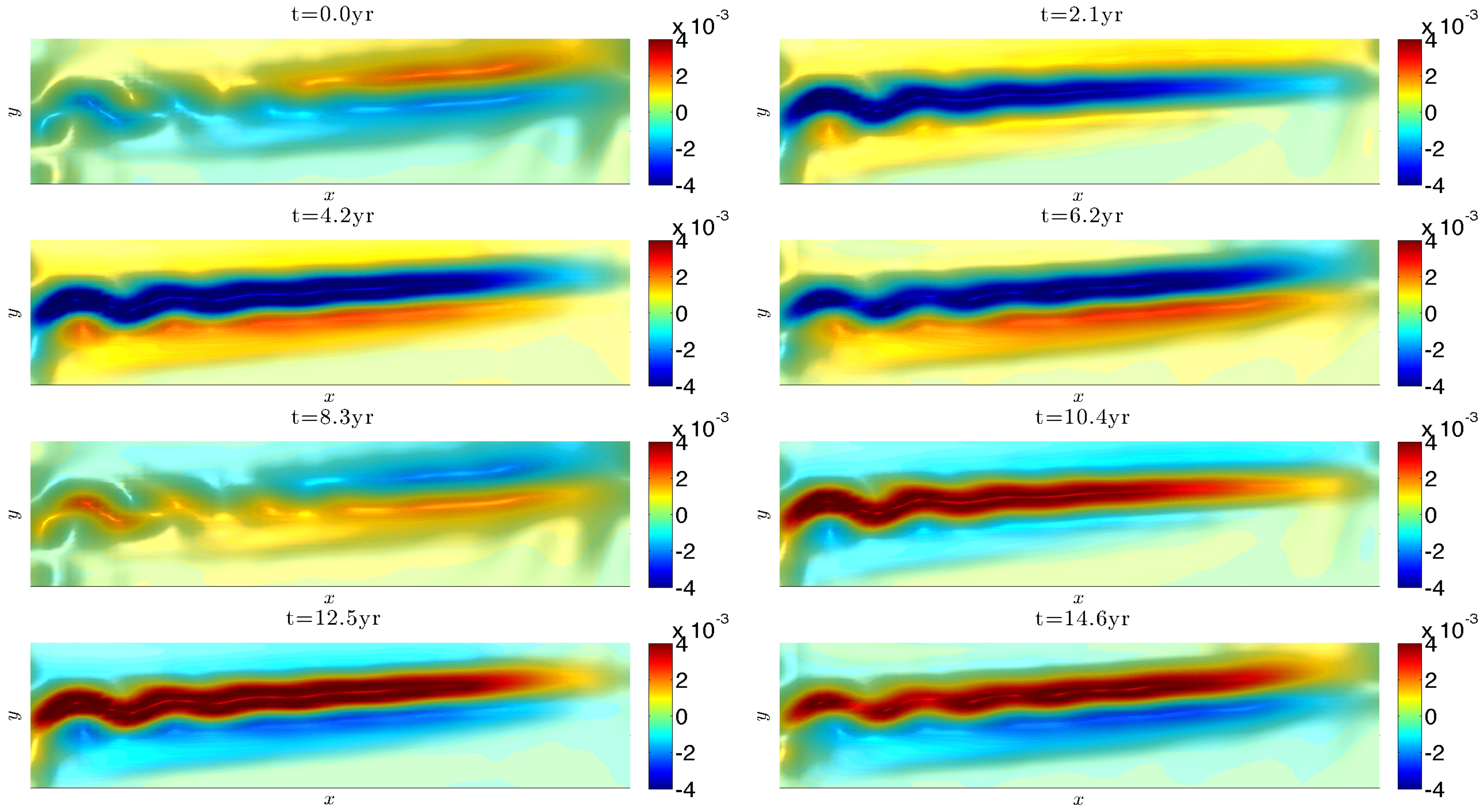
Figure 6.
Same as in Figure 5, but for the pair of DAHMs associated with the largest (top green dot in Figure 2) at the interannual frequency y (with period y) (cf. Figure 4).

Figure 7.
Decadal harmonic reconstruction component (HRC) and its reduced RP resonances for PC1: quasi-geostrophic (QG) model and multilayer Stuart-Landau model (MSLM). (a,b) show the sum of the first four HRCs on PC1 for the upper-layer stream function anomalies as simulated from the QG model (red curve) and its DAH-MSLM emulator (blue curve). In both panels, the PC1 is shown in black: in (b), PC1 is obtained after simulation of the DAH-MSLM emulator, whereas in (a), PC1 is obtained from simulation of the QG model. The HRCs are computed according to (23) in Section 4.2.2 below, from the corresponding simulated data. (c) shows the corresponding reduced RP resonances (see Appendix B) as estimated from HRCs shown in (a,b); colors match across panels (a–c).
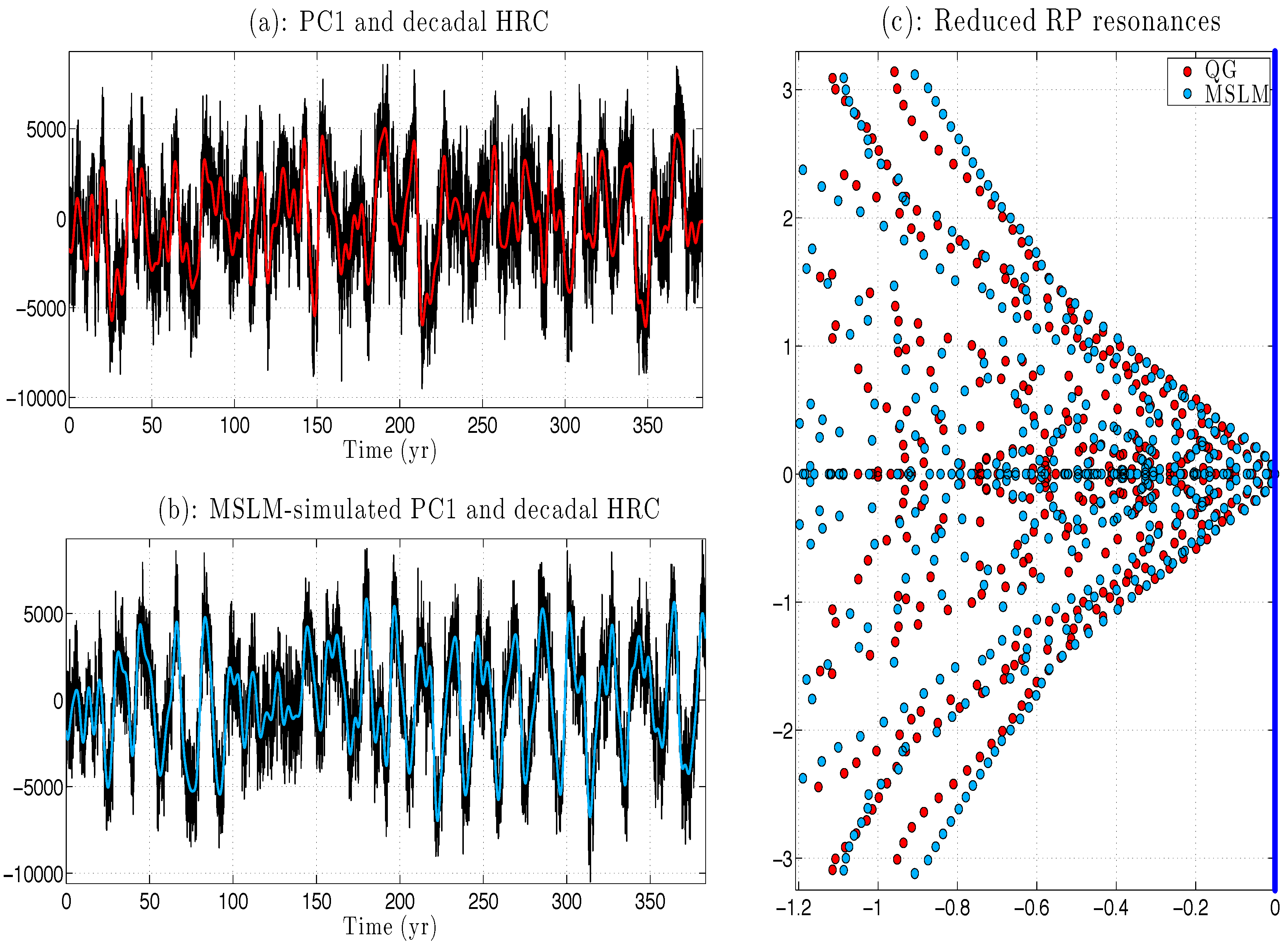
Figure 8.
Upper-level stream function anomalies and standard deviation: QG vs. MSLM. The QG’s standard deviation (SD) and its MSLM emulation are shown here in Panels (a,b), respectively, for the low-frequency range y. Panels (c,d) depict typical flow patterns underlying the SD patterns for the QG model and MSLM, respectively. Panels (e,f) (resp. (g,h)): same as for Panels (a,b) (resp. (c,d)), but for the intermediate frequency range y y.
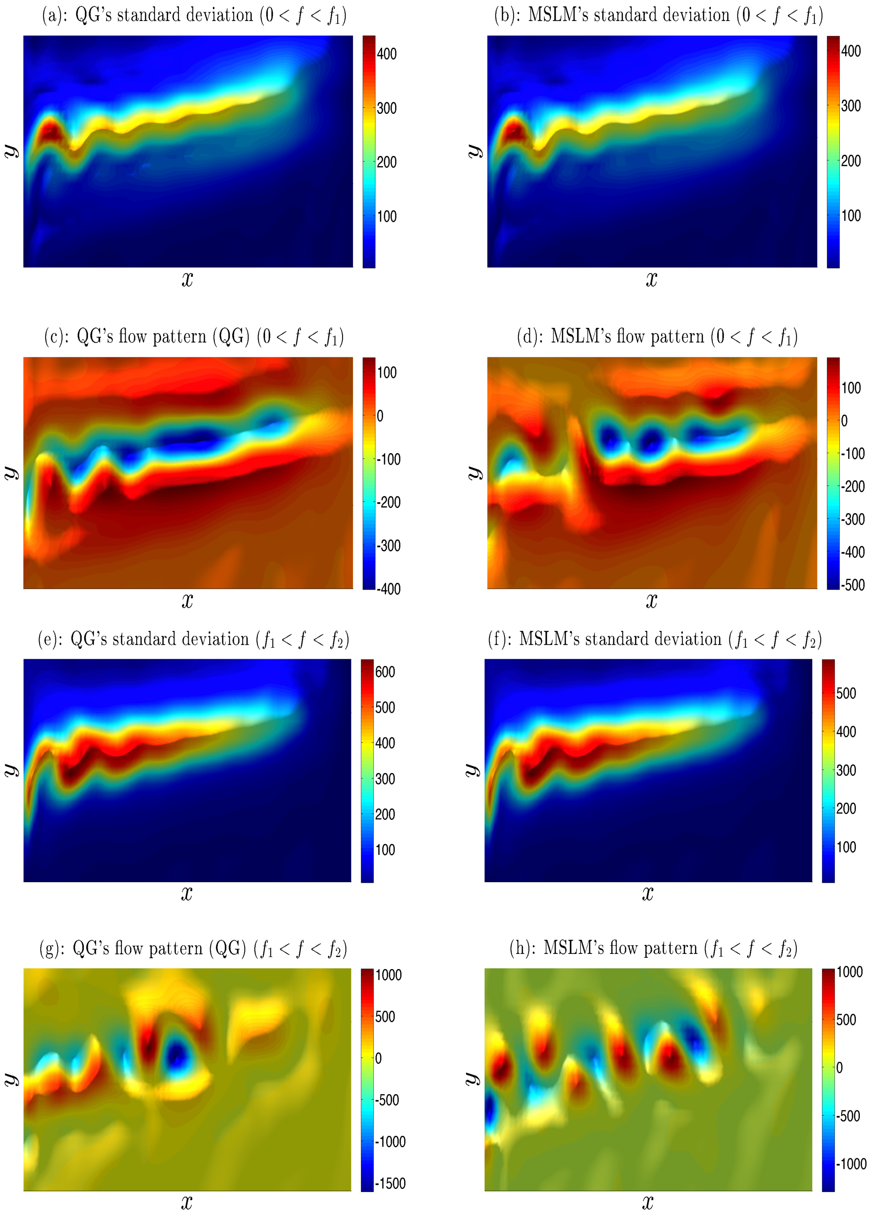
Figure 9.
Upper-level stream function anomalies and standard deviation: QG vs. MSLM. The QG’s standard deviation (SD) and its MSLM emulation are shown here in Panels (a,b), respectively, for the high-frequency range y y. Panels (c,d) depict typical flow patterns underlying the SD patterns for the QG model and MSLM, respectively. Panels (e,f) (resp. (g,h)): same as for Panels (a,b) (resp. (c,d)), but for the full range of frequencies y.

© 2018 by the authors. Licensee MDPI, Basel, Switzerland. This article is an open access article distributed under the terms and conditions of the Creative Commons Attribution (CC BY) license (http://creativecommons.org/licenses/by/4.0/).
Share and Cite
MDPI and ACS Style
Kondrashov, D.; Chekroun, M.D.; Berloff, P. Multiscale Stuart-Landau Emulators: Application to Wind-Driven Ocean Gyres. Fluids 2018, 3, 21. https://doi.org/10.3390/fluids3010021
AMA Style
Kondrashov D, Chekroun MD, Berloff P. Multiscale Stuart-Landau Emulators: Application to Wind-Driven Ocean Gyres. Fluids. 2018; 3(1):21. https://doi.org/10.3390/fluids3010021
Chicago/Turabian StyleKondrashov, Dmitri, Mickaël D. Chekroun, and Pavel Berloff. 2018. "Multiscale Stuart-Landau Emulators: Application to Wind-Driven Ocean Gyres" Fluids 3, no. 1: 21. https://doi.org/10.3390/fluids3010021