Design of a Novel μ-Mixer


1
Scientific Computing Department, STFC, Rutherford Appleton Laboratory, Didcot OX11 0QX, UK
2
Department of Chemical Engineering, Aristotle University of Thessaloniki, 54124 Thessaloniki, Greece
*
Author to whom correspondence should be addressed.
Fluids 2018, 3(1), 10; https://doi.org/10.3390/fluids3010010
Submission received: 15 December 2017
/
Revised: 10 January 2018
/
Accepted: 24 January 2018
/
Published: 28 January 2018
(This article belongs to the Special Issue Flow and Heat or Mass Transfer in the Chemical Process Industry)
Abstract
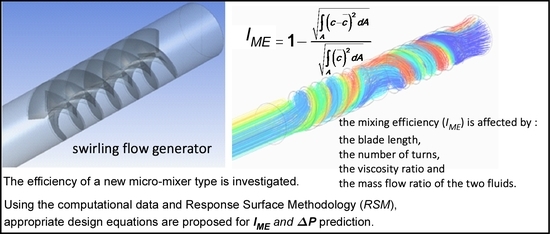
:In this work, the efficiency of a new μ-mixer design is investigated. As in this type of devices the Reynolds number is low, mixing is diffusion dominated and it can be enhanced by creating secondary flows. In this study, we propose the introduction of helical inserts into a straight tube to create swirling flow. The influence of the insert’s geometrical parameters (pitch and length of the propeller blades) and of the Reynolds number on the mixing efficiency and on the pressure drop are numerically investigated. The mixing efficiency of the device is assessed by calculating a number—i.e., the index of mixing efficiency—that quantifies the uniformity of concentration at the outlet of the device. The influence of the design parameters on the mixing efficiency is assessed by performing a series of ‘computational’ experiments, in which the values of the parameter are selected using design of experiments (DOE) methodology. Finally using the numerical data, appropriate design equations are formulated, which, for given values of the design parameters, can estimate with reasonable accuracy both the mixing efficiency and the pressure drop of the proposed mixing device.
1. Introduction
The increasing demand for more economical and, at the same time, more environmentally friendly production methods has led to the design of new process equipment. By the term micro-device (μ-device), we refer to devices with at least one characteristic dimension of the order of a few millimeters. Key benefits of μ-devices are the development of energy friendly, productive, and cost-effective performance processes which at the same time provide greater security. For example, μ-reactors—i.e., devices with characteristic dimensions in the submillimeter range—offer significant advantages over conventional reactors, such as increased safety and reliability, as well as better process control and scalability. Due to the small characteristic dimension of the conduit, the flow in μ-reactors is laminar. As the extent of the chemical reactions is governed by the slow diffusive mass transfer, which in turn is proportional to the interfacial area between the reacting phases, the μ-reactor design turns out to be a μ-mixer design problem. That is why mixing in small devices has been studied extensively in recent years.
In general, mixing is achieved by stirring, where, due to the turbulent nature of flow, mixing is accomplished by advection followed by diffusion. In μ-mixers, the flow is laminar and in this case depending on the way mixing is enhanced, μ-mixers are distinguished in passive and active ones. In active μ-mixers, an external source of energy is used [1]. Active micromixers are unfortunately difficult to integrate and, in general, they have a higher implementation cost. In passive μ-mixers, whose key advantage is the low operating cost, mixing efficiency is enhanced by incorporating parts that promote secondary flows (e.g., curved sections, backward or forward-facing steps). Several comprehensive reviews of μ-mixing devices and their principles can be found in the relevant literature [1,2,3,4,5,6]. As it has been reported [1,7,8,9] in the micro-scale, mixing can be improved by “chaotic advection”, which involves breaking, stretching, and folding of liquid streams leading to an increase of the interfacial contact area of the fluids.
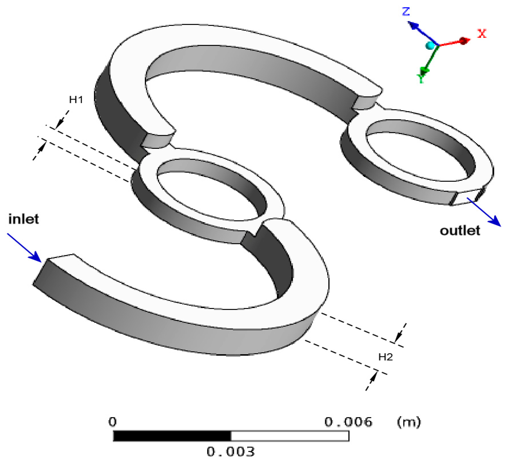
In our laboratory, the mixing efficiency of several types of passive μ-mixers was investigated both experimentally and numerically [5,6,7,10]. Figure 1 shows a typical passive μ-mixer (i.e., Dean-type) whose functional characteristics were studied in our previous works [7,10]. Static mixers that create swirl flow are common in the macro scale and recently the application of swirl inducing configurations has been also studied in the μ-scale [11]. It is also known [12] that static helical mixers are widely used in the chemical industry for in-line blending of liquids under laminar flow conditions and also that the geometric modification of their elements can significantly improve their mixing performance. Moreover, it is suggested [13] that the addition of obstructions as part of the channel geometry can be also beneficial to micromixer efficiency.
Motivated by the above, the purpose of this study is to investigate the possibility of using a helical insert (Figure 2) that enhances mixing by generating swirl flow. More precisely, our aim is to numerically assess the effect of the geometric parameters of the helical insert (pitch and length of the insert blades) (Figure 3) as well as the physical properties of the fluids to be mixed on both the mixing efficiency of the mixing device and the resulting pressure drop.
2. Numerical Methodology
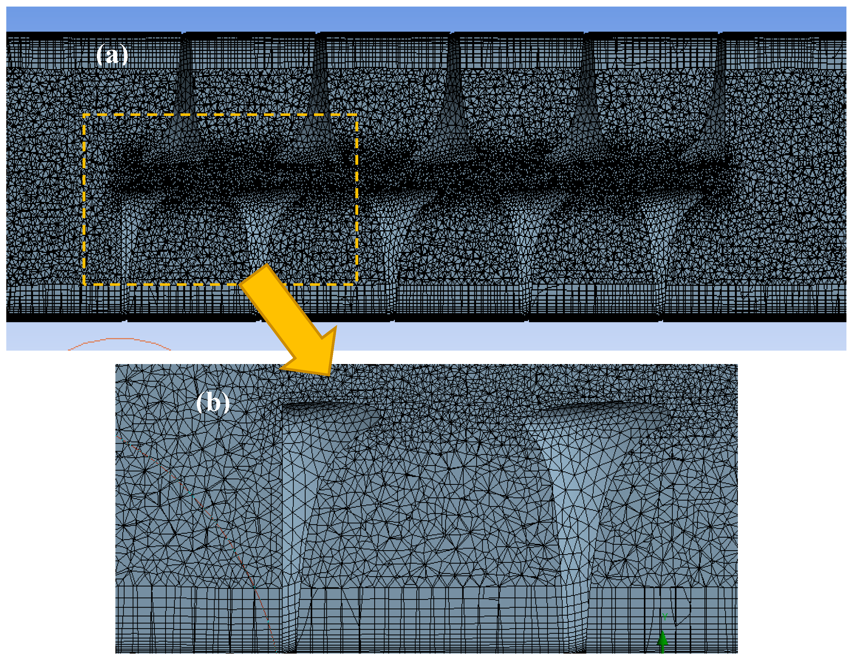
The velocity field was visualized using a computational fluid dynamics (CFD) code (ANSYS CFX 18.1, ANSYS, Inc., Karnosboro, PA, USA) while the computational geometry and the mesh were designed using the parametric features of ANSYS Workbench package. The μ-channel was modeled as a 3D computational domain. The simulations are performed using the ANSYS-CFX code, which includes the usual parts of a standard CFD code. The flow domain, constructed using the geometry section of the code, is presented in Figure 4. A grid dependency study was performed for choosing the optimum grid density. Detail of the insert is shown in Figure 4b, while the geometrical characteristics of the apparatus appear in Table 1.
In the present calculations, the computational fluid dynamics code uses the laminar flow model of ANSYS CFX and the high-resolution advection scheme for the discretization of the momentum equations. A pressure boundary condition of atmospheric pressure is set on the outlet port, while the convergence criterion is the mass-balance residual value is less than 10−9.
As the numerical diffusion in the CFD calculations can influence the accuracy of the calculations, a thorough grid dependency study was performed to ensure that the solution is independent of the grid density. Pressure drop between inlet and outlet of the device, as well as the water mass fraction profile at the outlet, were considered as metrics for the evaluation of the dependence of the grid density on the solution. The final grid parameters (minimum/maximum element size, number of divisions for the sweep mesh areas, etc.) for a representative screening run were used to define the meshing parameters for the rest of the simulation runs. Number of elements for all cases varied between 850,000 and 3,000,000 elements, approximately. Due to the small characteristic dimension of the conduit the flow is laminar (Re = 9–100) and hence the laminar flow model was selected. The boundary conditions imposed are:
- velocities of the two fluids, on each of the two semicircles comprising the inlet,
- non-slip boundary condition at all walls,
- zero relative pressure at the outlet.
Moreover, and for the sake of simplicity, it was assumed that one of the fluids, the base fluid, has the properties of water, while the diffusion coefficient between the two fluids equals the self-diffusion coefficient of water (1 × 10⁻⁹ m2/s).
Design parameters are declared as a mix of geometrical parameters and physical properties. Two geometrical design parameters, namely the number of turns, n, of the blade within the limits of the length of the insert, and the ratio, l/D, are used. The other variables applied are the ratios of density and dynamic viscosity for the two different mixing fluids as well as the ratio of their velocities at the entrance of the conduit. The finite volume method, a fully coupled solver for the pressure and velocity coupling, and the “high order” method to distinguish the momentum equations, all provided by ANSYS CFX, are used in the solver definition section [14]. Simulations were performed for a number of iterations that ensure a satisfactory reduction in residual mass and momentum (10−12).
The mixing efficiency over a cross-section A was quantified by calculating the Index of Mixing Efficiency, IME, proposed by Kanaris et al. [5], which is based on the standard deviation of mass fraction from the mean concentration over a cross section
where c is the mass fraction of the base fluid, in our case the water, in each cross-section unit (i.e., each grid element) and is the mean concentration of the same fluid over the whole cross-sectional area, A, of the device. Complete mixing is achieved when the volume fraction of the base fluid in each cross-section unit equals its mean mass fraction, , which must be calculated for each individual fluid pair by also taking into account the density of the mixing fluids:
A value of ΙΜΕ = 1 denotes perfect mixing, i.e., the variance from the optimal mass fraction is zero.
3. Results
3.1. Screening Experiments
To assess the effect of geometrical parameters on mixing efficiency, preliminary simulations—i.e., screening experiments—were performed. For the sake of simplicity, in these simulations both fluids had the properties of water. Initially only one helical insert was used and the simulations revealed that the length of the fluid path after the exit of the insert has only marginal contribution to the overall efficiency of the μ-mixer. Thus, to further improve mixing efficiency, a second insert was placed downstream and adjacent to the first one (Figure 5). The geometrical characteristics of the two inserts are identical, except that the blades of the two insert drive the fluid to opposite directions. A pipe extension, without any mixing promotion features, is placed downstream of the second insert, to allow the dissipation of vortices and a developed flow profile at the measuring cross section. The length-to-diameter ratio of this extension is selected to be around 10. As stated above, additional simulations ran for a length-to-diameter ratio of 20, showing borderline improvement (around +3%) of mixing efficiency and, therefore, it is considered that the originally selected ratio is adequate for the purpose of mixing characterization in this study. Also, as part of the initial screening simulations, a design with a single helical insert of up to twice the length of the proposed insert has been tested; results have shown that the addition of a counter-clockwise insert generally improves the mixing efficiency, with the magnitude being dependent on the geometry of the helical blades, as expected.
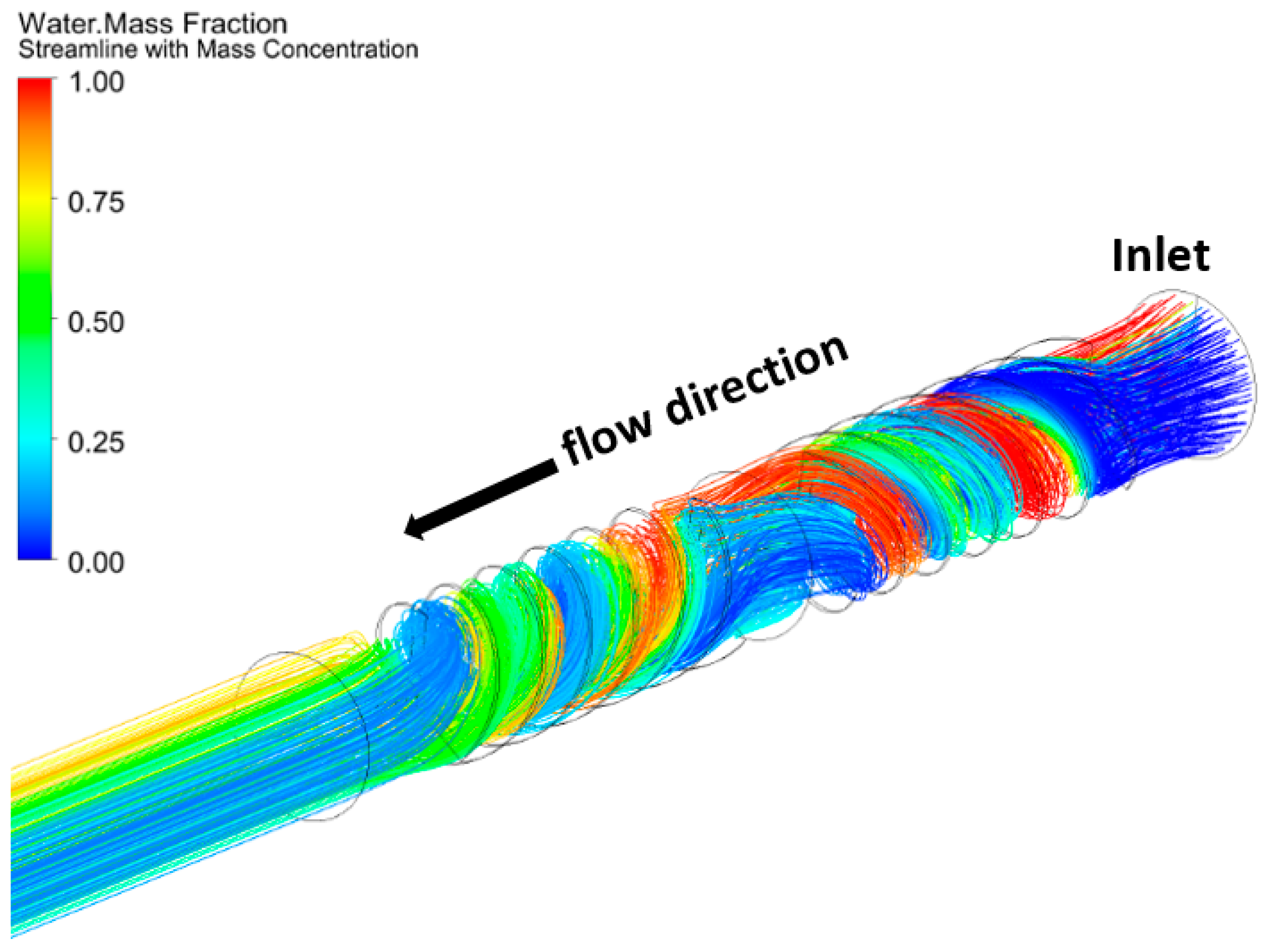
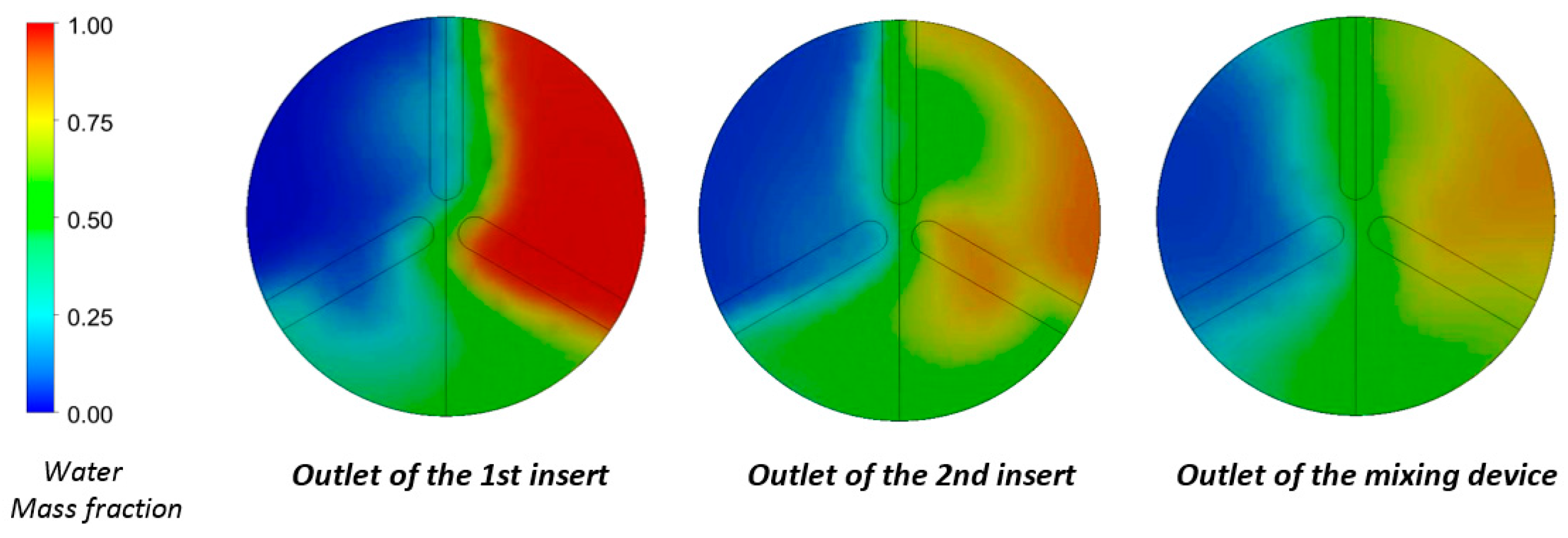
One of the initial screening runs, where the mixing fluids have identical properties and inlet velocities, while n = 3 and l/D = 0.2, is used to generate the typical results presented in Figure 5, Figure 6, Figure 7 and Figure 8. In Figure 5, the flow pattern (streamlines) along the proposed device with the two inserts is presented. It is evident that the addition of the second insert improves mixing. The effect of this addition is more clearly illustrated in Figure 6, where the mass fraction distribution of the base fluid is presented at three cross sections of the device, more precisely at the exit of the first and the second insert as well as at the outlet of the device.
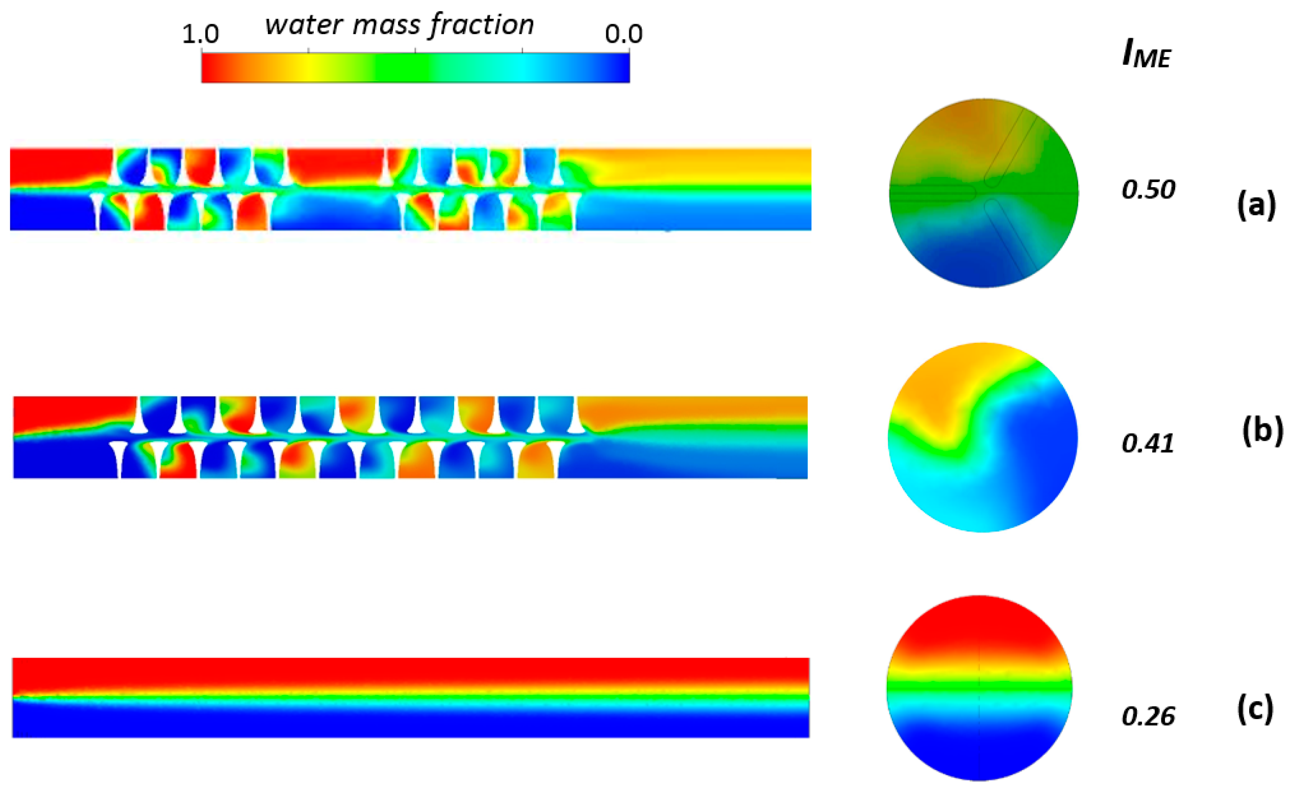
In Figure 7, the performance of the proposed device—i.e., the one with the two helical inserts—is compared with the one that contains a single helical insert with the same length as well as with that of a straight pipe, whose cross section and length are the same as that of the proposed device. For a certain set of the design parameters and for the same Re number (Rew = Re = 10) the use of the mixing device configuration almost doubles the value of the IME. The increase of the fluid velocity considerably affects the mixing efficiency, or equally the uniformity of the mass fraction distribution at the exit of the device (Figure 8). It is evident that, as it is expected, the mixing efficiency is mainly influenced by the value of Re, or equally the velocity of the fluid, which leads to more intense swirling flow, despite the fact that at lower velocities the contact time of the fluids is longer.
3.2. Parametric Study
The efficacy of the proposed mixing device was assessed by conducting a parametric study. However, to reduce the complexity of the problem, some variables—namely the length and the inside diameter of the mixing device as well as the position, the length, the radius and the angle between the blades of the insert—were kept constant (as presented in Table 1), while the two inserts are considered adjacent to each other. Also, for the sake of simplicity, the physical properties of one of the mixing fluids were assumed to be those of water, while the properties of the second fluid are variable and correspond to those of various types of water-based inks. For the same reason only two inserts were used, although it is evident that mixing will be further enhanced by inserting a series of inserts that would alternate the direction of flow. Table 2 presents the independent, dimensionless variables involved in the parametric study as discussed above together with their upper and lower bound values. Based on the values used, Re/Rew varies between 0.05 and 1.60.
The effect of the design parameters on the efficiency of the μ-device is investigated by performing a series of simulations for certain values of the design parameters chosen by employing the Box–Behnken method, i.e., an established design-of-experiments (DOE) technique that allows the designer to extract as much information as possible from a limited number of test cases [15]. For the present study, the number of design points dictated by the Box–Behnken method is 42 and presented in Table 3.
The generic form of a fully quadratic model with two design parameters, x1 and x2, is
The model includes the quadratic, the linear terms, and their interaction. To avoid overfitting, it is important that the researcher addresses the importance of each factor of the model. Additionally, it is also significant to take into account any possible insight regarding the potential form of the final equation and its non-linearity. For this reason, a different approach is followed in this case: the fitting approach uses the natural logarithms of the design parameters and responses. Based on the outcome, it is safe, within a certain degree of acceptable error, to ignore the quadratic terms and fit a model with only the linear terms and some of their interactions.
The following equation represents the proposed model
whose parameters can be calculated with regression based on response surface methodology; Y is the response, i.e., ΔP or IME, and cst is a constant. The annexed form of the final model would then be
A transform of the above model to include the Re ratio instead of the velocity ratio would be
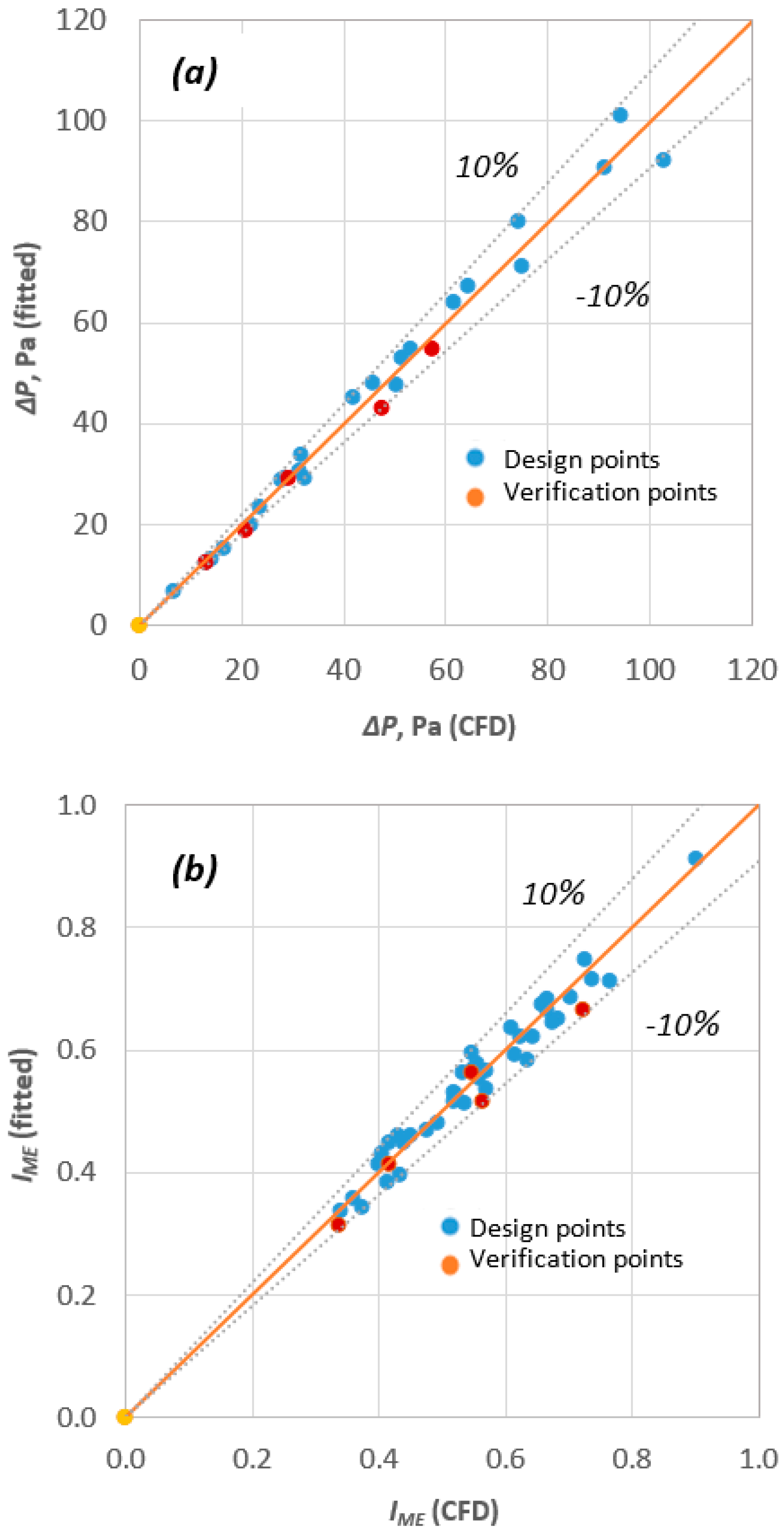
From Figure 9, where the values calculated using the proposed equations are compared with the CFD results, it is evident that they can predict with ±10% accuracy both ΔP (Figure 9a) and IME (Figure 9b) values. The validity of the proposed correlations is further examined by comparing them with CFD the results generated using the six ‘verification points’ presented in Table 5 and are also in agreement (Figure 9).
4. Conclusions
In this study, we have numerically investigated the mixing efficiency as well as the corresponding ΔP inside a novel type of μ-mixer. The device comprises two successive helical inserts that propel the fluid to opposite directions and induces mixing by generating swirling flow. Screening experiments reveal that the addition of the second insert improves mixing considerably. It was also found that for the range of Re numbers investigated, the resulting pressure drop is maintained at low levels (<150 Pa).
Appropriate ‘computational experiments’ were then conducted to investigate the effect of the various geometrical parameters of the novel μ-mixer, i.e., the one with the two inserts, and the parameters of the mixing fluids (physical properties and flow rate) on the mixing performance of the proposed device. Both the number of the required ‘computational experiments’ and the values of the design parameters were selecting using a DOE methodology. Using the data obtained from the ‘computational experiments’ correlations, which are able to predict the mixing efficiency and the associated pressure drop with ±10% accuracy, have been formulated.
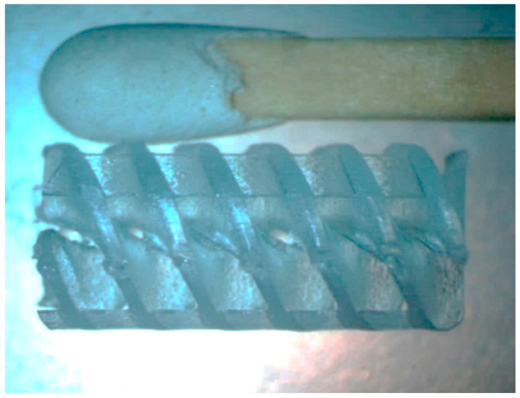
In the next stage of the study, experiments will be performed using a prototype helical insert that has been already constructed by 3D printing (Figure 10). The experimental data acquired using the device will be used for evaluating the CFD code. The aim is to provide a means of constructing the type of helical insert that would be more suitable for a given application.
Acknowledgments
The authors would like to thank Spiros V. Paras for his helpful comments.
Author Contributions
Aikaterini A. Mouza had the initial conception of this work; Athanasios G. Kanaris and Aikaterini A. Mouza designed the CFD experiments, acquired and analyzed the data, and interpreted the results; Athanasios G. Kanaris has provided insights on the improvement of computational performance for the required simulations; Aikaterini A. Mouza drafted the work and revised the manuscript. This work is not affiliated with the Science and Technology Facilities Council (STFC).
Conflicts of Interest
The authors declare no conflict of interest.
Nomenclature
| A | cross-section of the device | mm2 |
| b | blade pitch | mm |
| c | mass fraction in each cell of a cross-section A | dimensionless |
| mean concentration over a cross-section A | dimensionless | |
| D | diameter of the insert | mm |
| Dm | inside diameter of the device | mm |
| IME | index of mixing efficiency | dimensionless |
| l | blade length | mm |
| L | length of the insert | mm |
| Lm | total length of mixer | mm |
| n | number of turns of the insert | dimensionless |
| Re | Reynolds number of each liquid based on D | dimensionless |
| ΔP | pressure drop | Pa |
| μ | liquid viscosity | Pa s |
| ρ | liquid density | kg/m3 |
| φ | angle between blade | deg |
References
- Hessel, V.; Löwe, H.; Schönfeld, F. Micromixers—A review on passive and active mixing principles. Chem. Eng. Sci. 2005, 60, 2479–2501. [Google Scholar] [CrossRef]
- Nguyen, N.-T. Micromixers—A review. J. Micromech. Microeng. 2005, 15, R1. [Google Scholar] [CrossRef]
- Hardt, S.; Drese, K.S. Passive micromixers for applications in the microreactor and μTAS fields. Microfluid. Nanofluid. 2005, 1, 108–118. [Google Scholar] [CrossRef]
- Mansur, E.A.; Ye, M. A state-of-the-art review of mixing in microfluidic mixers. Chin. J. Chem. Eng. 2008, 16, 503–516. [Google Scholar] [CrossRef]
- Kanaris, A.G.; Stogiannis, I.A.; Mouza, A.A.; Kandlikar, S.G. Comparing the mixing performance of common types of chaotic micromixers: A numerical study. Heat Transf. Eng. 2015, 36, 1122–1131. [Google Scholar] [CrossRef]
- Aref, H.; Blake, J.R. Frontiers of chaotic advection. Rev. Mod. Phys. 2017, 89, 025007. [Google Scholar] [CrossRef]
- Kanaris, A.G.; Mouza, A.A. Numerical investigation of the effect of geometrical parameters on the performance of a micro-reactor. Chem. Eng. Sci. 2011, 66, 5366–5373. [Google Scholar] [CrossRef]
- Yuan, F.; Isaac, K.M. A study of MHD-based chaotic advection to enhance mixing in microfluidics using transient three dimensional CFD simulations. Sens. Actuators B Chem. 2017, 238, 226–238. [Google Scholar] [CrossRef]
- Aref, H. The development of chaotic advection. Phys. Fluids 2002, 14, 1315–1325. [Google Scholar] [CrossRef]
- Mouza, A.A.; Patsa, C.M.; Schönfeld, F. Mixing performance of a chaotic micro-mixer. Chem. Eng. Res. Des. 2008, 86, 1128–1134. [Google Scholar] [CrossRef]
- Huang, S.-W.; Wu, C.-Y. Fluid mixing in a swirl-inducing microchannel with square and T-shaped cross-sections. Microsyst. Technol. 2017, 23, 1971–1981. [Google Scholar] [CrossRef]
- Pahl, M.H.; Muschelknautz, E. Static mixers and their applications. Int. Chem. Eng. 1982, 92, 205–228. [Google Scholar]
- Rawool, A.S.; Mitra, S.K.; Kandlikar, S.G. Numerical simulation of flow through microchannels with designed roughness. Microfluid. Nanofluid. 2006, 2, 215–221. [Google Scholar] [CrossRef]
- Versteeg, Η.Κ.; Malasekera, W. Computational Fluid Dynamics; Longman Press: London, UK, 1995. [Google Scholar]
- Box, G.E.P.; Hunter, J.S.; Hunter, W.G. Statistics for Experimenters: Design, Innovation and Discovery, 2nd ed.; J. Wiley and Sons, Inc.: Hoboken, NJ, USA, 2005. [Google Scholar]

Figure 2.
Schematic of the μ-mixer.
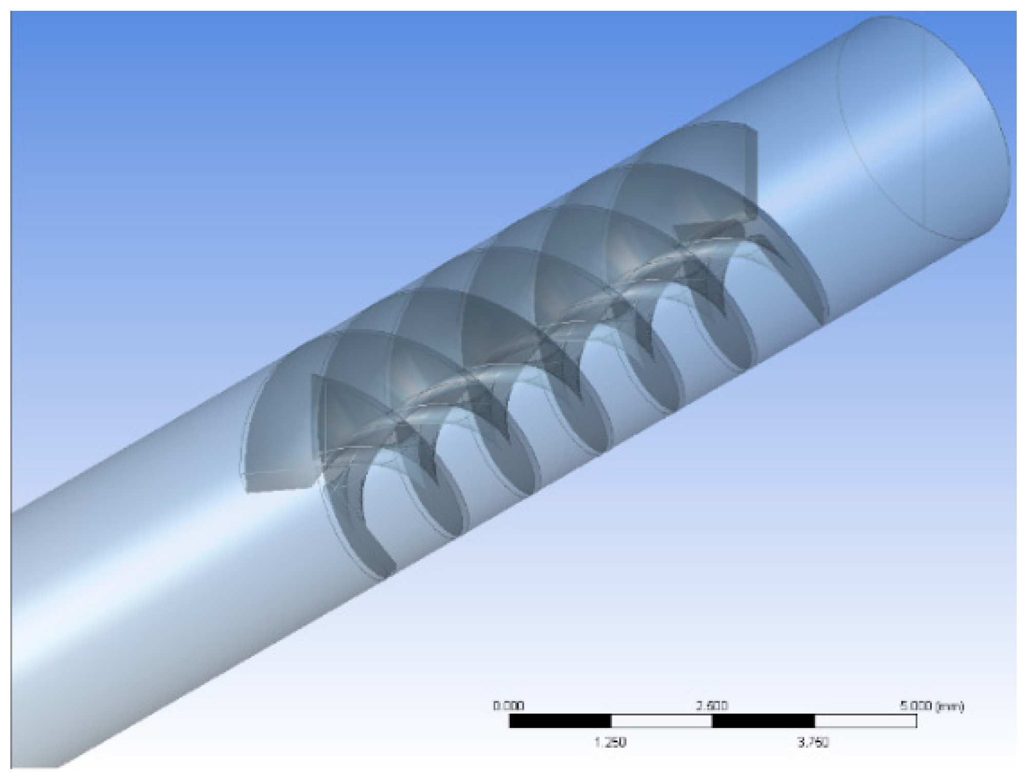
Figure 3.
Geometry of the swirl generator insert.
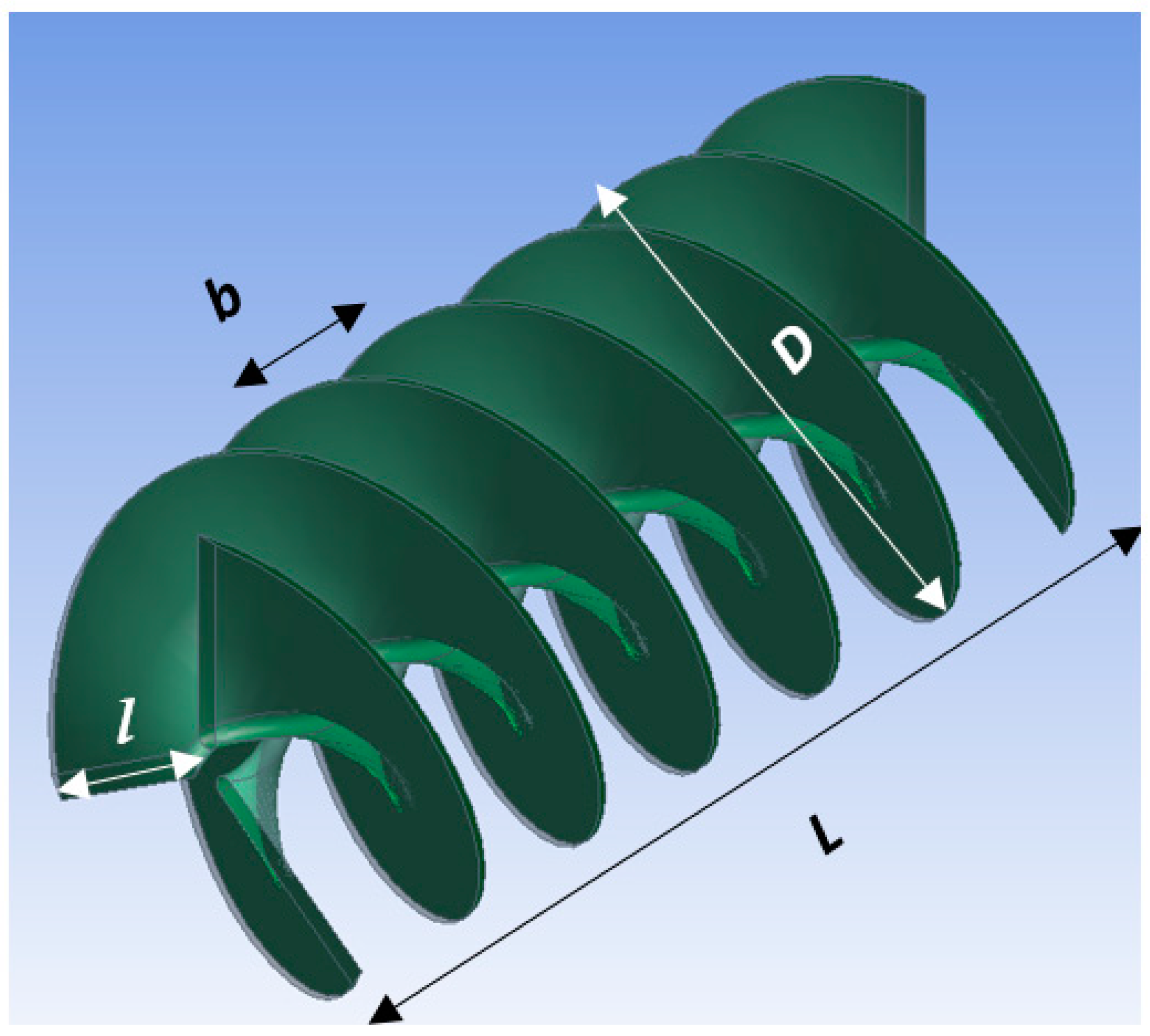
Figure 4.
(a) The flow domain and the grid and (b) grid detail.

Figure 5.
Typical mass concentration along streamlines (Re = Rew = 10).

Figure 6.
Mass fraction distribution at three cross sections of the device (Re = Rew = 10).

Figure 7.
Comparison of the mixing performance, in terms of mass fraction distribution at a plane along the axis and at the cross section at the outlet, as well as expressed as IME at the exit of the device: (a) device with two inserts; (b) device with one insert of double length; and (c) straight pipe (Re = Rew = 10).

Figure 8.
Effect of fluid velocity to the mixing efficiency at the outlet of the screening run device.
Figure 8.
Effect of fluid velocity to the mixing efficiency at the outlet of the screening run device.
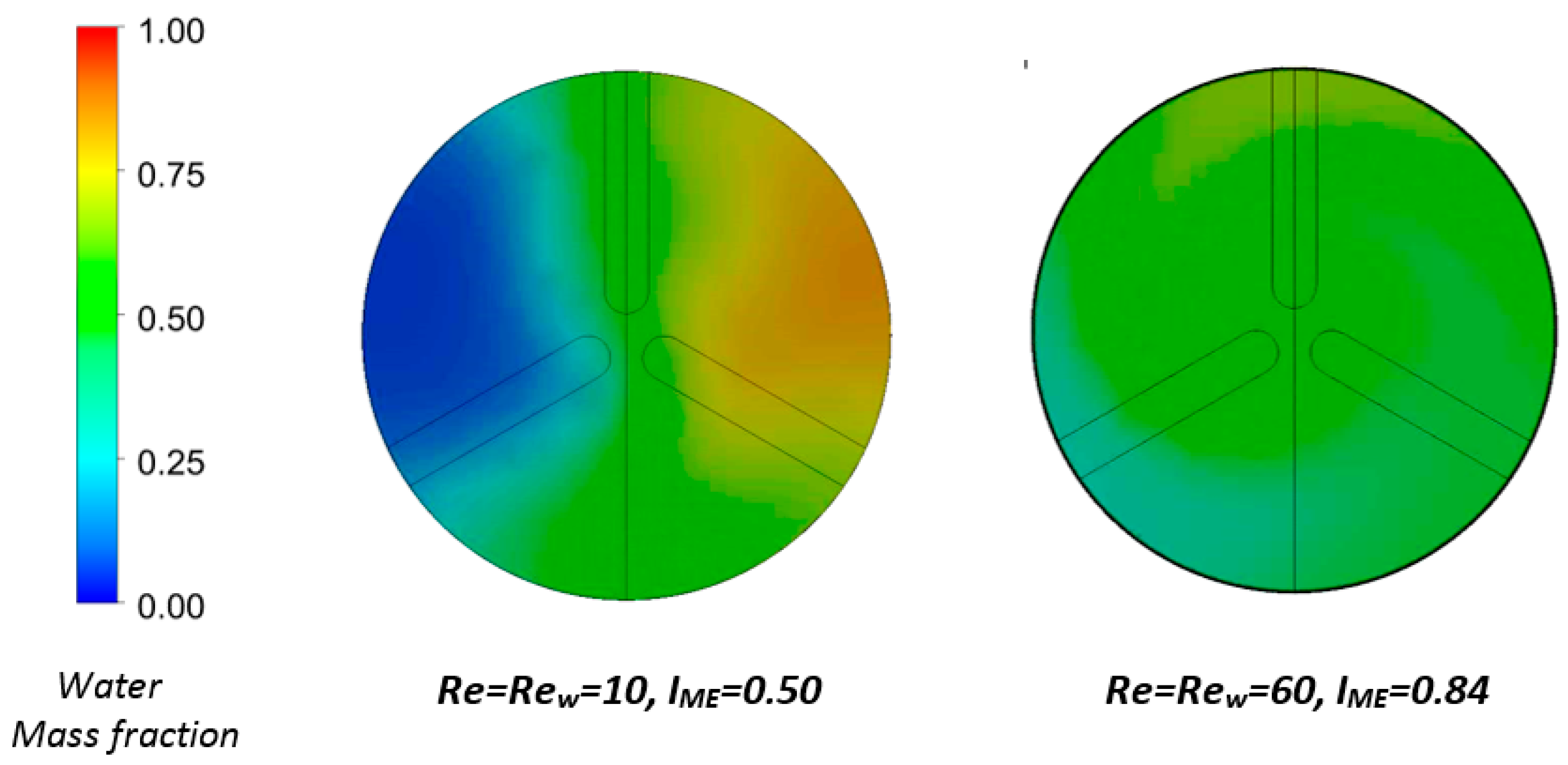
Figure 9.
Comparison between CFD and fitted values for (a) ΔP and (b) IME.

Figure 10.
The helical insert constructed by 3D printing.


Table 1.
Geometrical parameters of the mixing device
| Parameter | Value |
|---|---|
| Total length of the mixer, Lm | 52 mm |
| Internal diameter of the mixer, Dm | 3.1 mm |
| Diameter of the insert, D | 3.0 mm |
| Position of the insert (distance from mixer inlet), e | 3.0 mm |
| Length of the insert, L | 7.5 mm |
| Angle between blades, φ | 120° |
| Blade length, l | 0.60–1.74 mm |
| Blade pitch, b | 0.625–2.75 mm |
Table 2.
Constraints of the design variables
| Parameter | Lower Bound | Upper Bound |
|---|---|---|
| Number of turns, n | 1 | 3 |
| Blockage ratio, l/D | 0.20 | 0.58 |
| Dynamic viscosity ratio, μ/μw | 1.0 | 20.0 |
| Density ratio, ρ/ρw | 0.6 | 1.0 |
| Inlet velocity ratio, u/uw | 1.0 | 3.0 |
Table 3.
Design points for the simulation runs based on Box–Behnken design-of-experiments (DOE) methodology.
Table 3.
Design points for the simulation runs based on Box–Behnken design-of-experiments (DOE) methodology.
| Run# | Turns, n | l/D | μ/μw | ρ/ρw | u/uw | Run# | Turns, n | l/D | μ/μw | ρ/ρw | u/uw |
|---|---|---|---|---|---|---|---|---|---|---|---|
| DP01 | 3 | 0.20 | 10.5 | 0.8 | 2 | DP22 | 2 | 0.39 | 10.5 | 0.8 | 2 |
| DP02 | 1 | 0.20 | 10.5 | 0.8 | 2 | DP23 | 2 | 0.39 | 20.0 | 0.8 | 1 |
| DP03 | 1 | 0.39 | 10.5 | 0.6 | 2 | DP24 | 2 | 0.39 | 20.0 | 0.8 | 3 |
| DP04 | 1 | 0.39 | 1.0 | 0.8 | 2 | DP25 | 2 | 0.39 | 1.0 | 1.0 | 2 |
| DP05 | 1 | 0.39 | 10.5 | 0.8 | 1 | DP26 | 2 | 0.39 | 10.5 | 1.0 | 1 |
| DP06 | 1 | 0.39 | 10.5 | 0.8 | 3 | DP27 | 2 | 0.39 | 10.5 | 1.0 | 3 |
| DP07 | 1 | 0.39 | 20.0 | 0.8 | 2 | DP28 | 2 | 0.39 | 20.0 | 1.0 | 2 |
| DP08 | 1 | 0.39 | 10.5 | 1.0 | 2 | DP29 | 2 | 0.58 | 10.5 | 0.6 | 2 |
| DP09 | 1 | 0.58 | 10.5 | 0.8 | 2 | DP30 | 2 | 0.58 | 1.0 | 0.8 | 2 |
| DP10 | 2 | 0.20 | 10.5 | 0.6 | 2 | DP31 | 2 | 0.58 | 10.5 | 0.8 | 1 |
| DP11 | 2 | 0.20 | 1.0 | 0.8 | 2 | DP32 | 2 | 0.58 | 10.5 | 0.8 | 3 |
| DP12 | 2 | 0.20 | 10.5 | 0.8 | 1 | DP33 | 2 | 0.58 | 20.0 | 0.8 | 2 |
| DP13 | 2 | 0.20 | 10.5 | 0.8 | 3 | DP34 | 2 | 0.58 | 10.5 | 1.0 | 2 |
| DP14 | 2 | 0.20 | 20.0 | 0.8 | 2 | DP35 | 3 | 0.39 | 10.5 | 0.6 | 2 |
| DP15 | 2 | 0.20 | 10.5 | 1.0 | 2 | DP36 | 3 | 0.39 | 1.0 | 0.8 | 2 |
| DP16 | 2 | 0.39 | 1.0 | 0.6 | 2 | DP37 | 3 | 0.39 | 10.5 | 0.8 | 1 |
| DP17 | 2 | 0.39 | 10.5 | 0.6 | 1 | DP38 | 3 | 0.39 | 10.5 | 0.8 | 3 |
| DP18 | 2 | 0.39 | 10.5 | 0.6 | 3 | DP39 | 3 | 0.39 | 20.0 | 0.8 | 2 |
| DP19 | 2 | 0.39 | 20.0 | 0.6 | 2 | DP40 | 3 | 0.39 | 10.5 | 1.0 | 2 |
| DP20 | 2 | 0.39 | 1.0 | 0.8 | 1 | DP41 | 3 | 0.58 | 10.5 | 0.8 | 2 |
| DP21 | 2 | 0.39 | 1.0 | 0.8 | 3 | DP42 | 2 | 0.20 | 10.5 | 0.8 | 2 |
Table 4.
Response surface model parameters for (a) ΔP & (b) ΙΜΕ.
| Parameter | ΔP | ΙΜΕ |
|---|---|---|
| α | 0.817014 | 0.026161 |
| β | 5.456162 | −1.48235 |
| γ | 0.594749 | −0.34662 |
| δ | 0.312127 | −0.18884 |
| ε | 0.72966 | −0.42494 |
| ζ | 1.472507 | −0.99062 |
| η | −0.02689 | 0.097432 |
| θ | 0.014815 | −0.16046 |
| ι | 0.126574 | 0.092324 |
| cst | 5.91789 | −0.66962 |
Table 5.
Verification points
| Run# | Turns, n | l/D | μ/μw | ρ/ρw | u/uw |
|---|---|---|---|---|---|
| VP01 | 3 | 0.20 | 10.5 | 0.8 | 2 |
| VP02 | 1 | 0.20 | 10.5 | 0.8 | 2 |
| VP03 | 1 | 0.39 | 10.5 | 0.6 | 2 |
| VP04 | 1 | 0.39 | 1.0 | 0.8 | 2 |
| VP05 | 1 | 0.39 | 10.5 | 0.8 | 1 |
| VP06 | 1 | 0.39 | 10.5 | 0.8 | 3 |
© 2018 by the authors. Licensee MDPI, Basel, Switzerland. This article is an open access article distributed under the terms and conditions of the Creative Commons Attribution (CC BY) license (http://creativecommons.org/licenses/by/4.0/).
Share and Cite
MDPI and ACS Style
Kanaris, A.G.; Mouza, A.A. Design of a Novel μ-Mixer. Fluids 2018, 3, 10. https://doi.org/10.3390/fluids3010010
AMA Style
Kanaris AG, Mouza AA. Design of a Novel μ-Mixer. Fluids. 2018; 3(1):10. https://doi.org/10.3390/fluids3010010
Chicago/Turabian StyleKanaris, Athanasios G., and Aikaterini A. Mouza. 2018. "Design of a Novel μ-Mixer" Fluids 3, no. 1: 10. https://doi.org/10.3390/fluids3010010