3.1. Water Systems
A number of studies about the turbulent Schmidt number have dealt with the simulation of flow and tracer transport in open channels [
22,
23,
24,
25], while others have addressed those issues in contact or water tanks [
26,
27,
28,
29,
30,
31,
32,
33,
34,
35,
36], inclined negatively-buoyant discharges [
37], sediment-laden open channel flows [
38,
39,
40,
41,
42,
43,
44,
45,
46,
47,
48], density stratified turbulence [
49,
50] and T-junction mixing experiments [
51] (
Table 2). The terms “Exp” and “Num” mean the application of experimental and numerical methods, respectively, in each study.
Arnold et al. [
22] made extensive measurements in compound channel flow and were able to determine experimentally the values of
Sct. They found that
Sct varied from 0.1 to 1, with the vast majority of the values in between 0.5 and 0.9. This agreed well with the available data for free shear layers and plane jets (for which
Sct = 0.5) and for near-wall flows (
Sct = 0.9). The highest values were observed for rough flood plain conditions and high interaction effects, while the lower values were observed in the experiments with smooth flood plains and low interaction effects.
Djordjevic [
23] presented a mathematical model for transport processes in open-channel flow and the experimental validation of the model in rectangular and in compound channels. He experimentally determined a value of the eddy viscosity equal to the transverse mixing coefficient, implying that
Sct was close to unity for both section shapes. However, he argued that the extrapolation of this conclusion to natural flows is not straightforward.
Lin and Shiono [
24] presented a 3D numerical model to investigate transport processes of solutes in compound open channels. They solved numerically the RANS equations in conjunction with the linear and non-linear
k-
ε models to predict flow and turbulent parameters. Assuming a dimensionless transverse mixing coefficient of 0.134 and calculated values of the dimensionless eddy viscosity, they estimated
Sct = 0.72. However, they used for their simulations a value of 0.5, which corresponds to a larger eddy viscosity of 0.195, but this resulted in numerical predictions higher than the measured concentration data. They argued that this disagreement could be due to an incorrect prediction of the local value of the eddy viscosity in the hydrodynamic model or due to the assumption of a constant value of
Sct for the whole channel.
Simões and Wang [
25] developed a numerical model to simulate time-dependent turbulent flows in open channels, including the transport of dissolved materials. The turbulence closure was provided by two algebraic eddy-viscosity models. The three-dimensional turbulent flow field and the transport of a neutrally-buoyant solute in a compound channel were modelled. The numerical results were compared with experimental data. In the simulation, they used two values of
Sct: 0.5 and one. With the latter value, the results significantly underestimated the rate of spreading in the channel, and the concentrations were generally over-predicted. By using
Sct = 0.5, the numerical results showed a better agreement with the corresponding experimental values, but the vertical mixing rates were under-predicted. Hence, an anisotropic eddy diffusivity tensor with a
Sct of 0.5 for the horizontal mixing and one for the vertical mixing coefficient was used obtaining the best agreement with the experimental data.
In the study of tracer transport in a contact tank, [
30] and [
33] applied a value of one for
Sct. With
Sct = 1, [
33] obtained after several simulations the best agreement with the experimental data and stressed that the turbulent Schmidt number has a significant impact on the numerical simulations of tracer transport. Kim et al. [
31] and Zhang et al. [
34,
35,
36] compared the results from numerical simulations based on the RANS with those obtained using LES. They found that in a tank where the flow field is far from ideal plug flow conditions,
Sct = 0.3 was needed to match with the LES data in the concentration RTD (Retention Time Distribution) curve, whereas for
Sct = 1, the numerical results overestimated the LES data. This suggested that the best value for the
Sct could be related to the characteristics of the flow field in a contact tank [
53]. More recently, Angeloudis et al. [
26,
27,
28,
29] used
Sct = 0.7 to study the effect of tank geometry on the disinfection efficiency confirming the key role of this parameter in the reliable prediction of the tracer transport in a contact tank. The same value was adopted by Martínez-Solano et al. [
54] to study flow and concentration fields in a rectangular water tank [
32].
Oliver et al. [
37] applied the standard
k-ε model to achieve reasonable predictions for positively-buoyant vertical discharges before using it to simulate inclined negatively-buoyant discharges. The numerical results were compared with experimental data. The
k-
ε model was first implemented adopting standard parameter settings and
Sct equal to 0.9. To improve the agreement with the experimental data, the turbulent Schmidt number was calibrated to 0.6.
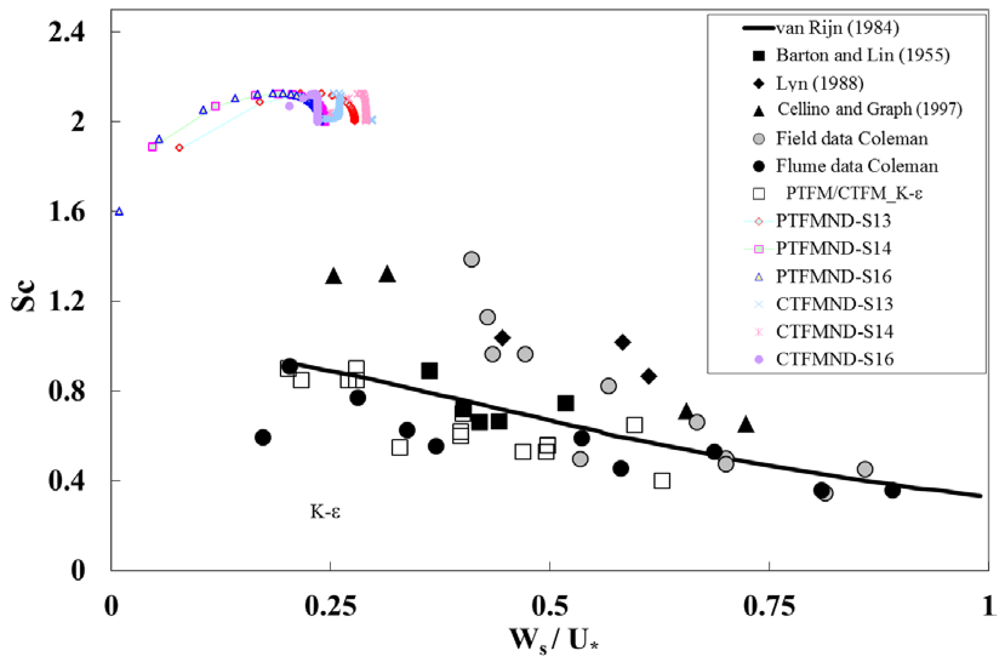
Several studies involved the case of sediment transport. The classical formula to determine the Schmidt number came from the work of van Rijn [
55]. By fitting a regression line in the experimental results, he suggested the following formula, which reflects the inertia of particles [
55]:
where
ws is the particle settling velocity and
u* is the shear velocity.
Equation (8) provides a value always less than one, applicable throughout the flow depth, and there is no explicit consideration of the type of bed. Graf and Cellino [
41] carried out experimental works to determine a depth-averaged value of
Sct by evaluating momentum and concentration diffusivity (Equation (2)) from measurements under laboratory conditions of instantaneous velocity and concentration profiles, obtained simultaneously by using an Acoustic Particle Flux Profiler (APFP). Considering also previous literature data, they concluded that for the suspension flows without bedforms
Sct > 1, whereas for the ones with bedforms as in natural waterways,
Sct < 1.
Adopting a constant value of
Sct and van Rijn pick-up function, Hsu and Liu [
42] calibrated the turbulent Schmidt number using the experimental results of [
56] and obtained
Sct = 0.7.
Amoudry et al. [
39] investigated the role of
Sct for a dilute two-phase sediment transport model with a
k-ε fluid turbulence closure. They first used a constant value of
Sct and found that the best fit with the experimental data was obtained with
Sct = 0.7 close to the bed and
Sct = 0.52 far from it. They concluded that describing the Schmidt number as a constant value might not be appropriate and that using a
Sct that depends on concentration generally gives the expected experimental dependence on the elevation from the bed. In doing so, they firstly considered, following [
55], that
Sct is typically less than unity because of centrifugal forces on the sediment particles, which cause the sediment particles to be thrown to the outside of the fluid eddies. Secondly,
Sct is expected to increase with the concentration because of the dynamic effect of the sediment itself, making it more difficult for sediment to be diffused. Thirdly, previous experimental data suggested a power law to relate the Schmidt number and sediment concentration. Finally, because an infinite sediment diffusivity is physically impossible, they forced
Sct to asymptotically approach a nonzero value as the concentration approaches zero. Hence, they proposed:
where
c is the sediment concentration and
c0 = 0.65 is the maximum possible sediment concentration (close-packing concentration), while
Sct-0 and
q are empirical constants. The application of Equation (9) resulted in an improvement of concentration predictions.
Muste et al. [
48] developed Particle Image Velocimetry-Particle Tracking Velocimetry (PIV-PTV) measurements to study the interaction between suspended particles and flow turbulent structures. They compared the traditional mixed-flow approach to sediment-laden flows that treats these flows essentially as flow of a single fluid, with a two-phase flow perspective. Two sets of experiments were conducted: one set with Natural Sand (NS) and the other set with Neutrally-Buoyant Sediment formed of crushed nylon (NBS). From the experimental data, they obtained values of the ratio between sediment to momentum diffusion coefficients quite different for the two datasets. The calculated
Sct values were much larger than one, namely from 1.4 to 2.11, for the NS flows, and much smaller than one, namely from 0.22 to 0.52, for the NBS flows.
Toorman [
52] derived Eulerian equations for the vertical flux and momentum of suspended particles in dilute sediment-laden open-channel flow in equilibrium using the two-fluid approach. Reynolds averaging was applied in order to allow validation of individual terms with experimental data. Moreover, he argued that progress in the prediction of suspended sediment transport requires a good closure for
Sct and that the available experimental data suggest that it varies over the entire depth. From the analysis of eddy viscosity and eddy diffusivity data obtained by using his new approach, Toorman concluded that it should be
Sct < 1. Finally, he obtained a new parameterization for
Sct as:
where
α is integral turbulence timescale factor,
cμ = 0.09 and
β0 is the inverse of the neutral
Sct., i.e., suspension-free turbulent Schmidt number. Using the experimental data from [
57], he concluded that the turbulent Schmidt number for suspension-free conditions is in the range from 0.5 to 0.8.
Bombardelli and Jha [
40] proposed, discussed and validated a theoretical and numerical framework for sediment-laden, open-channel flows, which was based on the Two-Fluid-Model (TFM) equations of motion. Within the umbrella of the RANS equations, they applied
k-
ε-type closures (standard and extended) to account for the turbulence in the water phase. They additionally reported and discussed the values of
Sct found to improve the agreement between predictions of the distribution of suspended sediment and the experimental data. Their results suggested values of
Sct smaller than one for dilute mixtures, indicating that the diffusivity of momentum of the carrier fluid, i.e.,
νt, is smaller than the diffusivity of sediment. In particular, they obtained a value for
Sct in the range from 0.56 to 0.7 depending on the experimental dataset, which was in agreement with those from Van Rijn equation ranging from 0.601 to 0.668.
Jha and Bombardelli [
44] assessed the performance of diverse turbulence closures in the simulation of dilute sediment-laden, open-channel flows. Under the framework proposed in [
40], they discussed the simulation results obtained by applying the Reynolds stress model (RSM), the algebraic stress model (ASM), the
k-
ε and the
k-
ω models (in their standard and extended versions), paired with each member of the framework. To assess the accuracy of the models, they compared numerical results with the experimental data from several datasets. They concluded that
Sct is the key parameter to obtain satisfactory predictions of sediment transport in suspension. In particular, following the findings presented in [
40], they noted that for
Sct = 0.56, the results from ASM, the
k-
ε and the
k-
ω models were in agreement with the experimental data, while RSM deviated from the data, and it was in agreement only for
Sct = 0.42. In general, for the
k-
ε model, the fitting with experimental data was obtained with
Sct in the range from 0.4 to 0.9, depending on the experimental dataset. Jha [
43] investigated under the framework of the RANS equation the effect of inertia on the transport of particle-laden open channel flow. He analyzed the sensitivity to a range of particle size, density and concentration and observed that
Sct decreased with the increase in particle size in the case of flow with high particle density. For low particle density, the maximum concentration of the particles at the channel bed governed the values of the Schmidt number required to match the experimental data.
Absi [
38] addressed the profile of suspended sediments concentration over ripples. He argued that field and laboratory measurements showed a contrast between an upward convex profiles for fine sands and an upward concave profiles for coarse sands. Second, the application of a 1D vertical gradient diffusion model with
Sct = 1 resulted in good predictions of the concentration profile for fine sediments, but it fails for coarse sand. Hence, he proposed to consider
Sct as a function of the distance from the bed and of an additional parameter, which is a function of the settling velocity.
Huang et al. [
49] applied the buoyancy-modified
k-
ε model to the saline density currents and dilute sediment-laden turbidity currents. A calibrated value of 1.3 for
Sct improved overall matches between the experimental data and the numerical simulation, especially near the bed. On the other hand,
Sct = 0.9 generally produced lower simulated concentration for this near-bed region. Therefore, they suggested that in stratified turbidity currents and density currents, the turbulent Schmidt number should be greater than one. This could be interpreted as a decrease in the turbulent diffusivity in order to take into account the decay of turbulence due to density stratification.
Huq and Stewart [
50] performed experiments on stably-stratified turbulence in a water tunnel. Turbulent velocity, density fields and buoyancy flux were measured to determine the turbulent Schmidt number
Sct.
Sct values were found to be dependent on two parameters, the Richardson number
Ri, i.e., the strength of stratification, and
T* representing the non-dimensional eddy turnover timescale.
T* is defined as the ratio of the advective time scale to the time scale of energy transfer from large to small eddies. The dependence of
Sct on
T* had not been identified previously. For large values, i.e.,
T* ≈ 10,
Sct is independent of
Ri and approached the value for neutral stratification, i.e.,
Sct = 1. In contrast, for small values, i.e.,
T* ≈ 1,
Sct increased with
Ri. He finally argued that the variation of
Sct with
T* explains the large scatter of
Sct values observed in atmospheric and oceanic datasets as a range of values of
T* occur at any given
Ri.
Experimental data obtained at an adiabatic T-junction, using wire-mesh sensors and the concentration of dissolved ions as the transport scalar, were used by Walker et al. [
51] to validate steady-state CFD calculations with some widely-used turbulence models, such as the k-ε model, the Menter’s Shear Stress Transport (SST) model and the Menter Baseline (BSL) Reynolds stress model. By using the default value for
Sct of 0.9, turbulent mixing was underestimated regardless of the model used. A decrease of
Sct down to 0.2 and 0.1 improved the agreement, although some qualitative differences in the shape of the concentration profiles remained. Hence, better results were obtained by increasing of the model coefficient
Cμ in the
k-ε model, leading to an improvement of both concentration and velocity profiles.
3.2. Atmosphere Systems
A large number of studies has been carried out to identify the best value for the turbulent Schmidt number to be applied in the numerical simulation of scalar transport in atmospheric systems. A first group of studies was aimed at estimating the most proper value for
Sct and at identifying the impact of
Sct on the numerical results [
54,
58,
59,
60,
61,
62,
63,
64,
65,
66,
67,
68] (
Table 3). Again, the terms “Exp” and “Num” mean the application of experimental and numerical methods, respectively, in each study.
Koeltzsch [
66] reviewed some previous experimental investigations and found that most authors use a constant value for
Sct ranging from 0.5 to 0.9.
Flesch et al. [
63] used measurements of pesticide emission from a bare soil to calculate
Sct. During their experiments,
Sct averaged 0.6, with large variability between observation periods that could not be correlated to atmospheric conditions. Some of this variability was due to measurement uncertainty, but they concluded that it also reflected true variability in
Sct.
Wilson [
69] measured vertical fluxes and concentration differences above a spring wheat crop to derive the turbulent Schmidt number for water vapor and carbon dioxide based on concentration differences between intakes 2.55 and 3.54 m above the ground. During nearly-neutral stratification, he obtained a
Sct = 0.68 ± 0.1 for water vapor and
Sct = 0.78 ± 0.2 for carbon dioxide.
Tominaga and Stathopoulos [
67] reviewed a number of previous studies related to the application of optimum values of
Sct for engineering flow fields relevant to atmospheric dispersion, such as jet-in-cross flow, plume dispersion in boundary layer and dispersion around buildings. They found that the optimum values for
Sct were widely distributed in the range of 0.2–1.3, and the specific value selected had a significant effect on the prediction results. Since the optimum values of
Sct largely depended on the local flow characteristics, they recommended that
Sct should be determined by considering the dominant effect in the turbulent mass transport in each case.
Riddle et al. [
68] simulated the atmospheric boundary layer flow and plume dispersion from an isolated stack for neutral stability and flat terrain situations. They compared the CFD results about the spread of gas plume with the predictions from the Atmospheric Dispersion Modelling System (ADMS), a well-tested and validated quasi-Gaussian model. They used
Sct = 0.7, but found that the CFD predictions were significantly higher (exceeding a factor of two) than expected values. By reducing
Sct to 0.3 to increase the plume dispersion, the predicted ground level concentrations were improved, but the horizontal plume spread was still significantly less than expected.
Di Sabatino and Buccolieri [
61] compared the CFD simulations with the predictions from a well-validated Gaussian model for the case of dispersion due to the presence of a buildings array. They found the best results for low and high frontal area density when using
Sct = 0.7 and 0.4, respectively.
Blocken et al. [
58] presented the results of a numerical study of pollutant dispersion in the neutrally-stable Atmospheric Boundary Layer (ABL) for three case studies: plume dispersion from an isolated stack, low-momentum exhaust from a rooftop vent on an isolated cubic building model and high-momentum exhaust from a rooftop stack on a low-rise rectangular building with several rooftop structures. They concluded that numerical results were quite sensitive to the value of
Sct, which was ranging from 0.3 to 1.
Chavez et al. [
59] carried out numerical simulations of pollutant transport in urban environments, for both isolated buildings and a group of buildings, using
Sct equal to 0.1, 0.3 and 0.7. They found a strong influence of
Sct on CFD simulations of pollutant transport for the isolated building configurations; however, variations of
Sct had less impact on assessing pollutant dispersion in the presence of adjacent buildings.
Mokhtarzadeh-Dehghan et al. [
54] applied the RANS approach to simulate the dispersion of a heavier-than air gas from a ground level line source in a simulated atmospheric boundary layer. They considered three cases for a Richardson numbers
Ri* of 0.1, 7 and 16. The results showed significant sensitivity to the value of
Sct, that was in the range from 0.7 to 2.5 depending on the value of
Ri*. By optimizing the value of
Sct as a linear function of the Richardson number, they obtained close comparisons between the predicted and measured parameters.
Ebrahimi and Jahangirian [
62] presented a new analytical formulations for the calculation of the most effective parameters in the Gaussian plume dispersion model; for comparison, CFD simulations were carried out for single stack dispersion on a flat terrain surface. They used
Sct = 0.7.
Chen et al. [
60] applied the RANS approach with the standard
k-
ε model to study turbulence and dispersion of gaseous substances in urban areas on building to city block scales. They used both a standard value of
Sct = 1.0 and a corrected value based on the concentration data collected in a wind tunnel experiment. However, deviation of the concentration between the simulation with the corrected
Sct and the wind tunnel experiments was observed due the constant
Sct assumption used in the CFD model.
Hassan et al. [
65] presented a modified multi-scale turbulence approach to allow the resolved field to adaptively influence the value of
Sct in the RANS sub-filter model. As the simulation proceeded, averaged resolved turbulent mass and momentum viscosities were calculated, and
Sct was defined based on their ratio. This approach resulted in a better agreement with the experimental data for a supersonic crossflow.
Galeazzo et al. [
64] conducted high-resolution measurements using particle image velocimetry combined with laser-induced fluorescence to validate simulations ranging from simple steady-state RANS to sophisticated LES. They used a constant value of
Sct in the range from 0.3–0.9 to gain a better reliability of numerical results. However, they pointed out that
Sct should be considered as a vector quantity.
A second group of studies investigated the question if
Sct is a constant or it is varying inside the flow domain [
66,
70,
71,
72]. Koeltzsch [
66] carried out wind tunnel experiments in a turbulent boundary layer above a flat plate. The data showed a strong dependence of
Sct, which was in the range from 0.3 to 1, on the height within the boundary layer. These experimental data corresponded well with values reported previously when the height used is normalized by the boundary layer thickness, suggesting that
Sct should be not considered as a constant in the flow domain.
Goldberg et al. [
70] proposed an approach based on an extension of the [
20] algebraic Reynolds stress model and relies on Reynolds stresses’ anisotropy. The approach used these stresses to algebraically build velocity-scalar correlations, which were the starting point for a variable
Sct formulation.
Ross [
71] performed numerical simulations of scalar transport in neutral flow over forested hills using both a 1.5-order mixing-length closure scheme and LES. He found that the common assumption that momentum and scalars are transported in the same way is not valid within and just above the canopies, with strong variations in
Sct in the vertical direction and across the hill.
Shi et al. [
72] investigated the performances of six RANS models and one LES model in predicting both weakly- and strongly-stratified jets. The velocity, turbulent kinetic energy and Reynolds stress distributions were examined. They proposed an equation for
Sct based on the local velocity gradient and density gradient with the objective to improve the simulation of scalar variables, such as the density difference distributions in the jets.


 ,
, 


