3.1. Mesh Independence Tests
To ensure that the simulation results are independent of grid size, different computational meshes were inspected. This is done by running cases with increasing number of grid cells until the simulation results did not change with the use of progressively finer grids.
Table 1 lists the properties of six different grids with varying density that have been inspected for the flow pattern around the NACA 0015 airfoil with zero flap deflection. This table lists some details of the grids, including the total number of cells, the number of nodes
and
placed, respectively, in the x and y directions and the maximum, minimum and average values of non-dimensional normal distance from the wall,
for each grid. It is observed that all of the grids inspected have considerably low
values, particularly Grids III–VI, to sufficiently resolve the viscous sub-layer.
Table 2 provides more details on the distribution of cells for different inspected meshes along the
x and
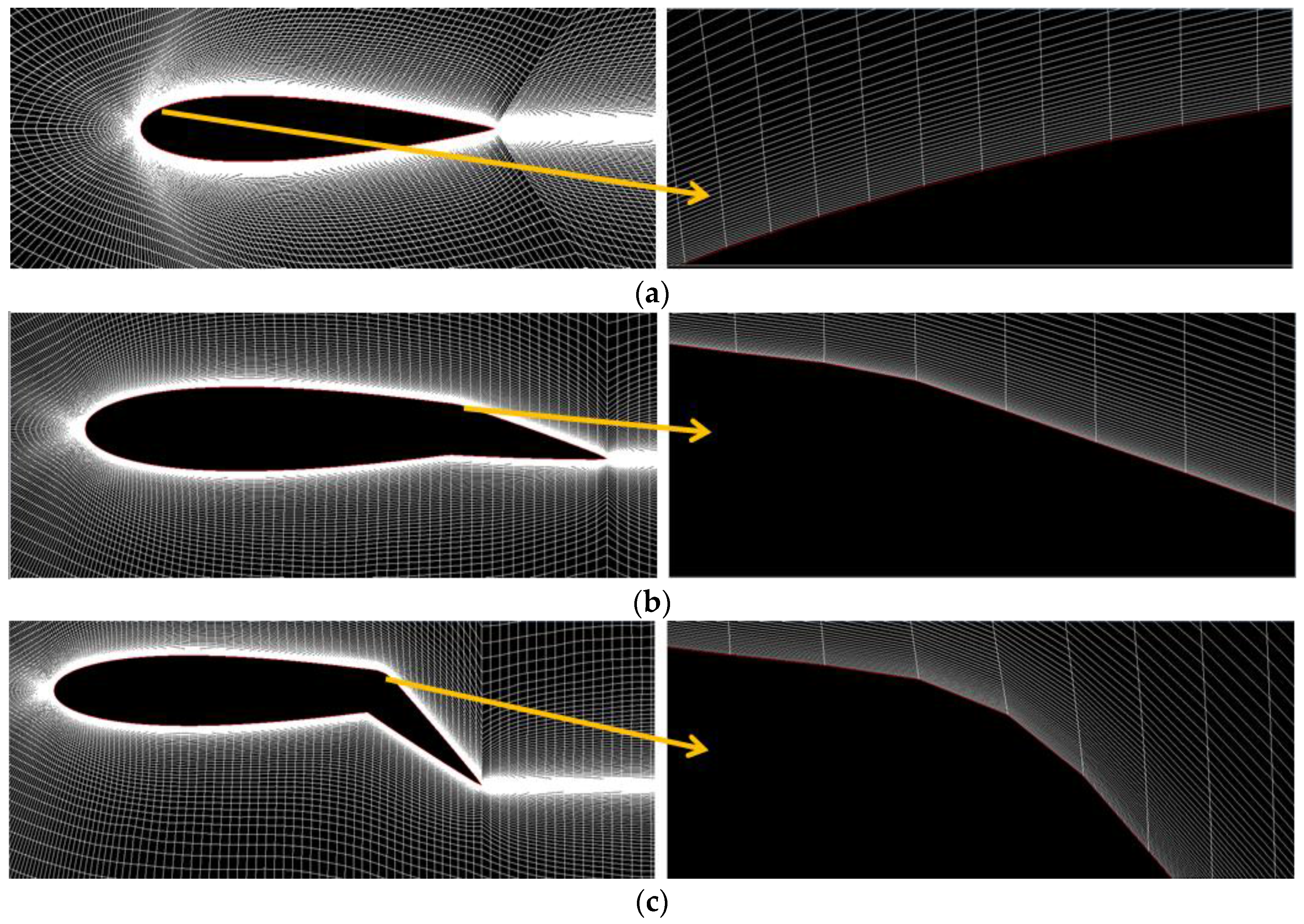
y directions. To have a better control of the distribution of the mesh, the airfoil body was divided into two parts; the front portion of the airfoil, which extends from the leading edge up to 30% of the chord length, and the rear portion of the airfoil, which includes the rest of the airfoil body. The wake region extends from the airfoil trailing edge up to the right far-field end. In each case, the first 30% of the airfoil was meshed with non-uniform grid spacing along the
x-axis, while the last 70% of the airfoil meshed with uniform grid spacing. The number of grid cells located in the airfoil rear portion is more than three-times that located at the front part.
The mesh size near the airfoil surface is a critical parameter for proper simulation of boundary layer flow properties. The size of the first cell height near the wall
was estimated based on the physical properties of the fluid used and the selected values of the non-dimensional normal distance from the wall
.
Table 3 gives values for estimated size of this first cell height as a fraction of airfoil chord length. The mesh growth factor that controls the transition of cell size and specifies the increase in element size for each succeeding layer is found to be 1.2.
In this section, the grid inspection studies for flows at Reynolds numbers of 10
5 and 10
6 are performed. The results of the two-equation realizable
k-ε model of Shih et al. [
20] were compared with those of the one-equation closure model of the Spalart–Allmaras (SA). The SA model was developed mainly for simulating aerodynamic flows. This model solves the modeled transport equation for the kinematic eddy (turbulent) viscosity [
26]. The results obtained from SA and
R-
k-ε numerical models were compared with the experimental data of Rethmel [
27].
Table 4 and
Table 5 show the predicted values of the lift coefficients for six different meshes by using the Spalart–Allmaras (SA) and the
R-
k-ε turbulence models for Re = 10
5 and 10
6, respectively. It is apparent that the realizable
k-ε solutions obtained by Grids IV, V and VI are in good agreement with the experimental data. Despite the fact that the number of cells in Grid VI is approximately 3.7-times that of Grid IV, these grids provided nearly the same results for the lift coefficient. It is also seen that the SA model yields significantly higher
values compared to the experiments. Regardless of the turbulence model used, the numerical results for these last three grids remain almost the same with increasing the number of cells from Grid IV–Grid VI.
The last step in the grid convergence inspection was focused on the analysis of the distribution of the pressure coefficient along the airfoil chord, as well as the velocity profiles on the upper surface of the airfoil in some selected sections.
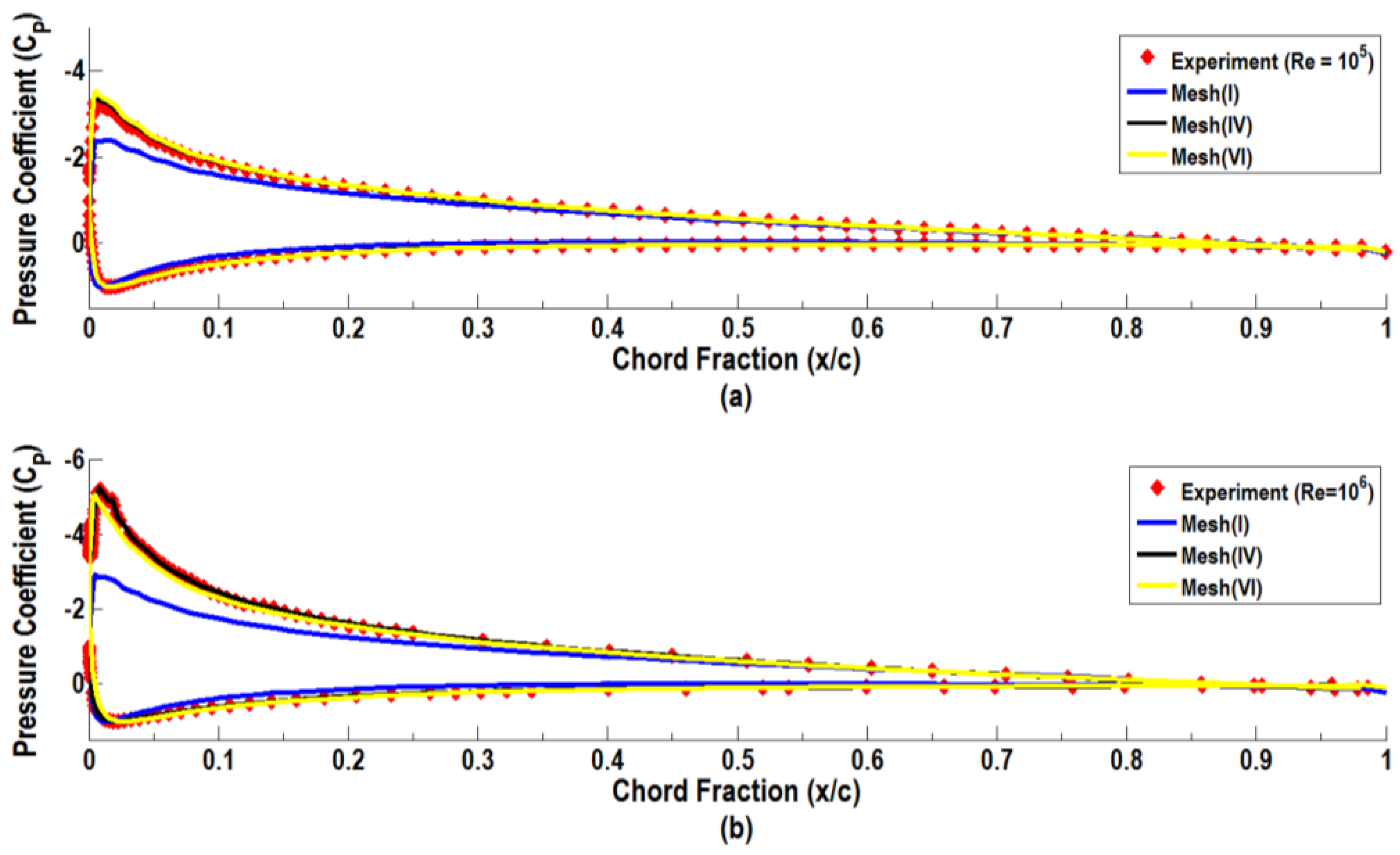
Figure 4 presents the chordwise distributions of the pressure coefficient (
Cp) profile for the airfoil predicted by Grids I, IV and VI using the
R-
k-ε turbulence model for α = 12°, δ = 0° and Re = 10
5 (a) and Re = 10
6 (b). Here, the predicted distributions of the pressure coefficient are compared with the experimental data of Rethmel [
27]. It is seen that the model predictions for the pressure coefficient are generally comparable with the experimental data. In particular, the predictions obtained by Grids IV and VI are very close to each other and to the distribution of the experimental data for both Reynolds numbers.
Figure 5 shows the velocity profiles on the upper surface of airfoil at the 20% cord location from the leading edge as predicted by the realizable
k-ε model using Grids I, IV and VI for α = 12° and δ = 0° for Re = 10
5 and Re = 10
6. The vertical axis (
y) in
Figure 5 denotes the vertical distance from the surface of the airfoil as a fraction of the chord length. It is seen that the model predictions for Grids IV and VI are almost identical. That is, further refinement of Grid IV does not have a noticeable effect on the velocity profile.
The presented grid sensitivity analysis shows that the model predictions with the use of Grids IV and VI are very close to each other and to the experimental data. Due to the high computational cost associated with the use of Grid VI, Grid IV with a total number of 103,192 cells was used in the subsequent analyses.
3.2. NACA 0015 Airfoil with Zero Flap Deflection
The airflow properties around the NACA 0015 with zero flap deflection are first studied, and the corresponding distributions of static pressure and velocity magnitude at different incidence angles are evaluated and compared with the published numerical results and/or experimental data.
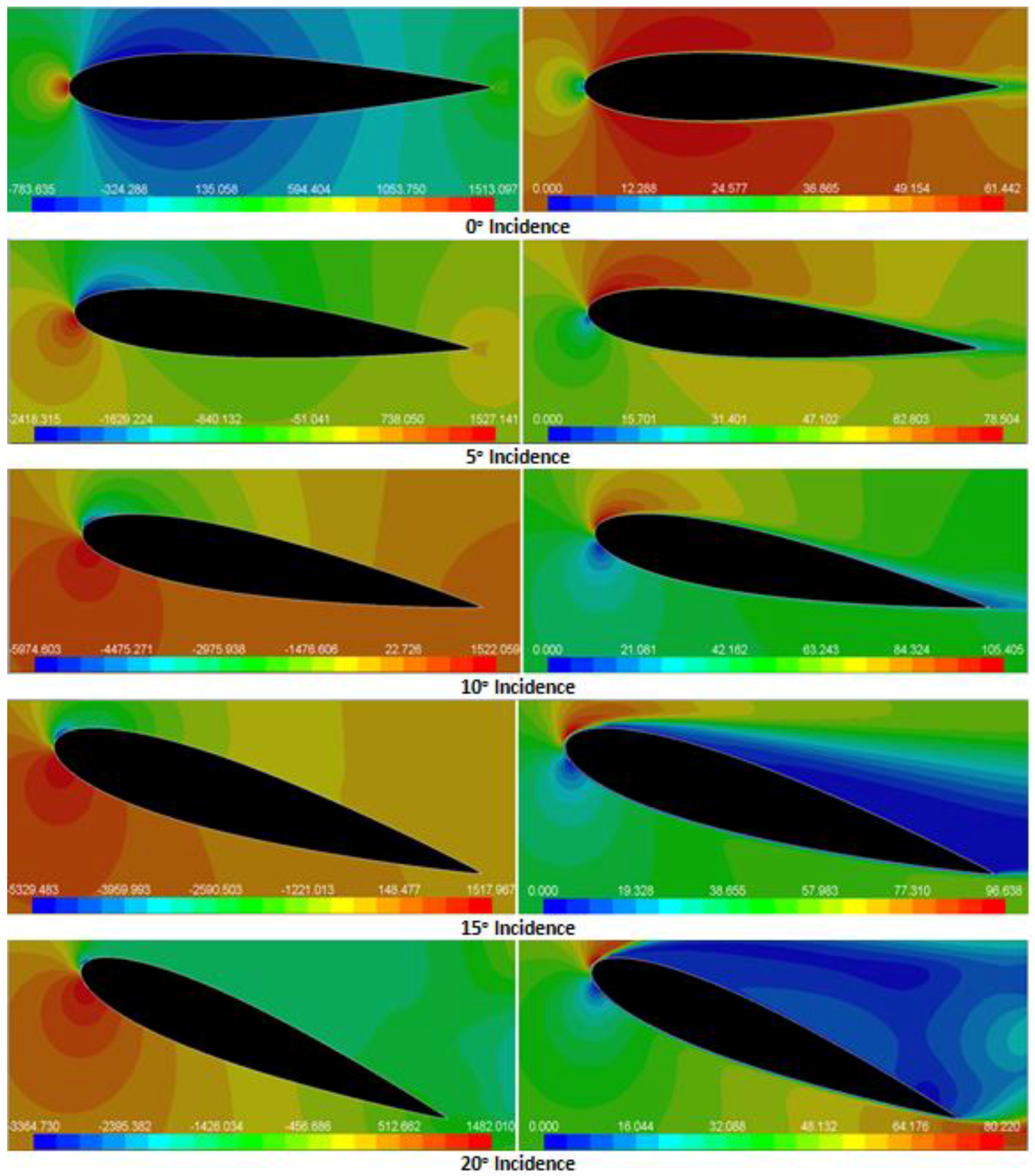
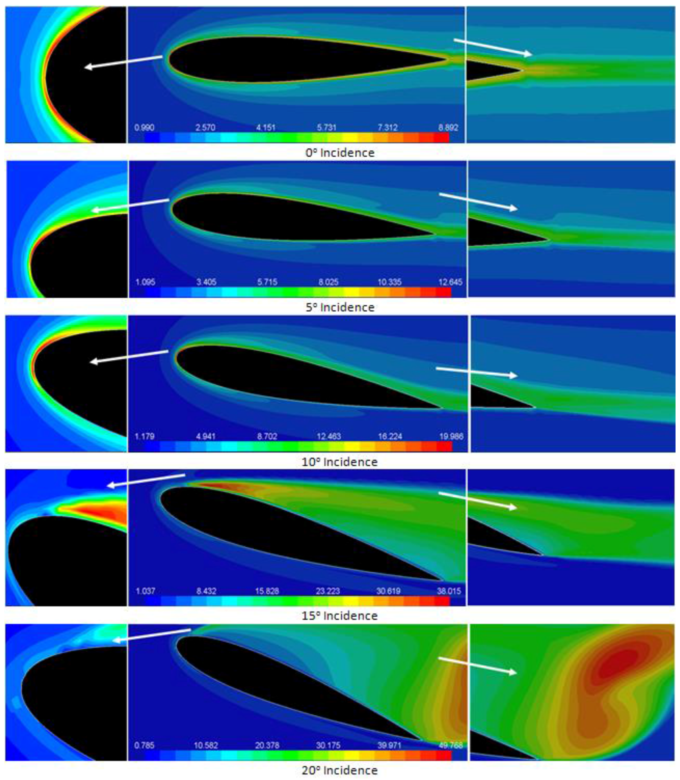
Figure 6 shows the static pressure and velocity magnitude contours around the NACA 0015 airfoil for a few selected incidence angles. As NACA 0015 is a symmetric airfoil, at zero incidence angle, the static pressure and velocity distribution over the airfoil are symmetric, which results in zero lift force and a stagnation point, exactly at the nose of the airfoil. There are regions of accelerated flows over and under the airfoil that reach the highest speed at the airfoil maximum thickness point. The velocity is high (marked by red spots) in the low pressure region and vice versa. The maximum pressure occurs at the stagnation point when the velocity is zero.
At an incidence angle of 5°, the contours of static pressure over the airfoil become asymmetric; the pressure on the upper surface becomes lower than the pressure on the lower surface; regions of high pressure on the airfoil lower surface become dominant; and a lift coefficient of 0.531 is generated due to the pressure imbalance.
Figure 6 shows that as the angle of attack increases, the stagnation point is shifted towards the trailing edge on the bottom surface; hence, it creates a low velocity region at the lower surface of the airfoil and a high velocity region on the upper side of the airfoil. Thus, the pressure on the upper side of the airfoil is lower than the ambient pressure, whereas the pressure on the lower side is higher than the ambient pressure. Therefore, increasing the incidence angle is associated with the increase of the lift coefficient, as well as the increase of the drag coefficient. This increase in the lift coefficient continues up to a maximum, after which the lift coefficient decreases.
It is also seen that the flow field around the airfoil varies markedly with the incidence angle. In addition to the changes in velocity and pressure distributions, the properties of the boundary layer flow along the airfoil surface also change. At low incidence angles up to about 12°, the boundary layer is fully attached to the surface of the airfoil, and the lift coefficient increases with angle of attack, while the drag is relatively low. With the increase of incidence angle, the boundary layer is thickened. When the incidence angle of the airfoil is increased to about 13° or larger, the adverse pressure gradient imposed on the boundary layers become so large that separation of the boundary layer occurs. A region of recirculating flow over the entire upper surface of the airfoil forms, and the region of higher pressure on the lower surface of the airfoil becomes smaller. Consequently, the lift decreases markedly, and the drag increases sharply. This is a typical condition in which the airfoil is stalled.
For a further increase of the airfoil incidence angle to 20°, the stagnation point shifts significantly further towards the trailing edge on the bottom surface. The recirculating flow region becomes dominant and covers the entire upper surface of the airfoil, and the airflow is fully separated from the upper surface of the airfoil. This leads to further reduction of the lift force and a severe increase of the drag force.
The air flowing along the top of the airfoil surface experiences a change in pressure, moving from the ambient pressure in front of the airfoil, to a lower pressure over the surface of the airfoil, then back to the ambient pressure behind the airfoil. The region where fluid must flow from low to high pressure (adverse pressure gradient) could cause flow separation. If the adverse pressure gradient is too high, the pressure forces overcome the fluid inertial forces, and the flow separates from the airfoil upper surface. As noted before, the pressure gradient increases with incidence angle, and there is a maximum angle of attack for keeping the flow attached to the airfoil. If the critical incidence angle is exceeded, separation occurs, and the lift force decreases sharply.
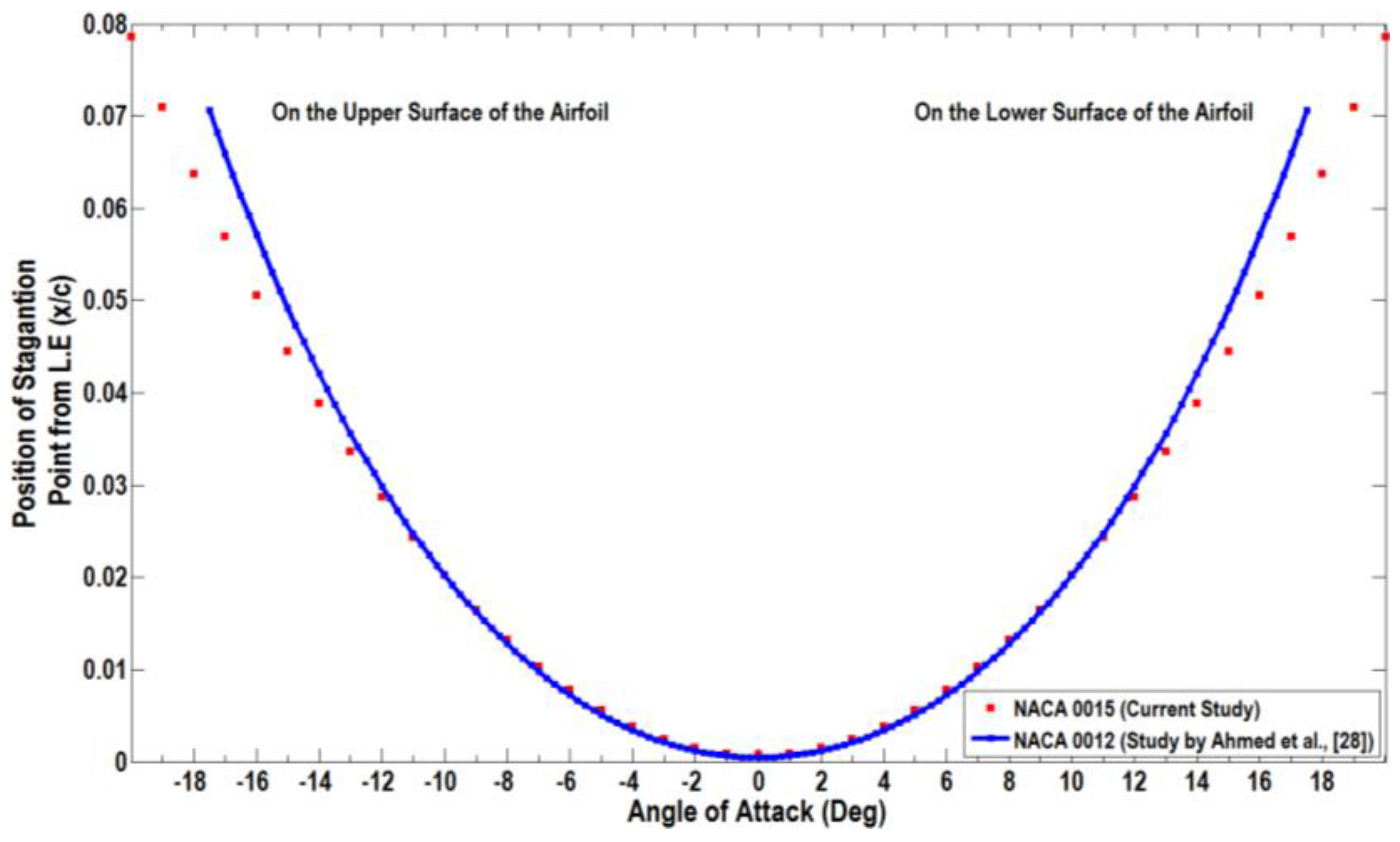
Figure 7 shows how the predicted position of the stagnation point varies for different angles of attack. It is apparent that with positive angle of attack (AoA) the stagnation point moves toward the trailing edge on the lower surface of the airfoil, while this movement would be on the upper surface of the airfoil at negative angles. The variation of the stagnation point position with the angle of attack obtained in this study is compared with the results obtained by Ahmed et al. [
28] for the NACA 0012 airfoil. Although the NACA 0012 airfoil is thinner, the present results match well up to an AoA of 12° and then follow the same trend.
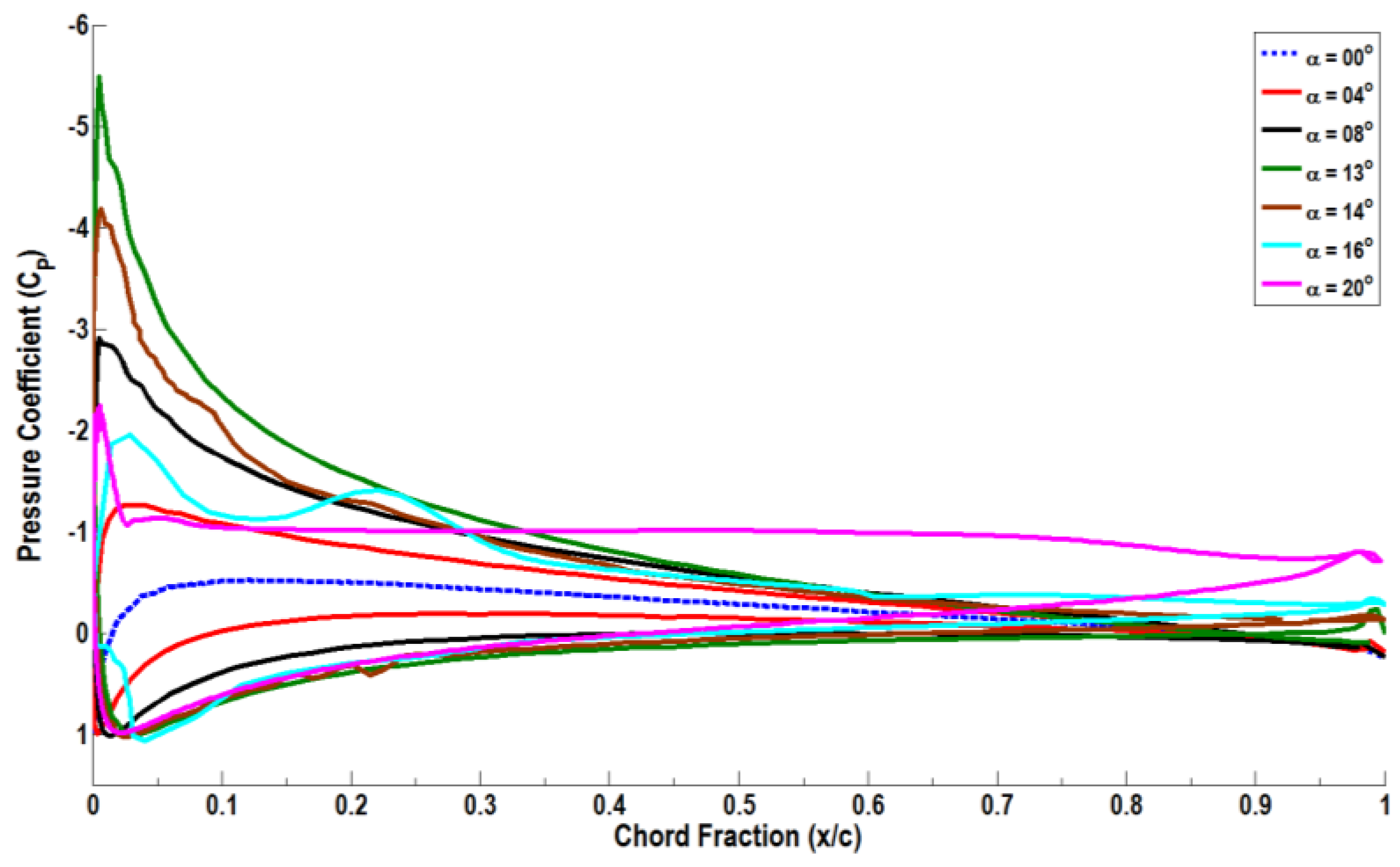
Figure 8 presents the chordwise distributions of the pressure coefficient (
Cp) profile for the airfoil at some selected incidence angles. For small angles of attack, the
Cp distribution is characterized by a negative pressure peak near the leading edge on the suction side. Beyond this point, the
Cp value gradually increases along the chord of the airfoil. On the pressure side of the airfoil, the
Cp value reaches a maximum of
Cp = 1 at the stagnation line. This point is near the leading edge, but shifts slightly depending on the incidence angle. Further down the chord length of the airfoil, the pressure side
Cp value increases gradually until it equals the suction side value at the trailing edge.
Figure 8 also shows that the flow remains attached to the suction surface up to α = 13° after which flow begins to separate. The separation line starts near the trailing edge and moves forward toward the leading edge as incidence increases. The flow becomes fully separated over almost the entire chord of the airfoil for α greater than 15°. For α > 13°, the maximum
Cp negative value decreases on the airfoil upper side, and a pronounced shift of the stagnation position toward the trailing edge is found. This situation continues until α = 17°, at which the
Cp value starts to vary in an irregular manner.
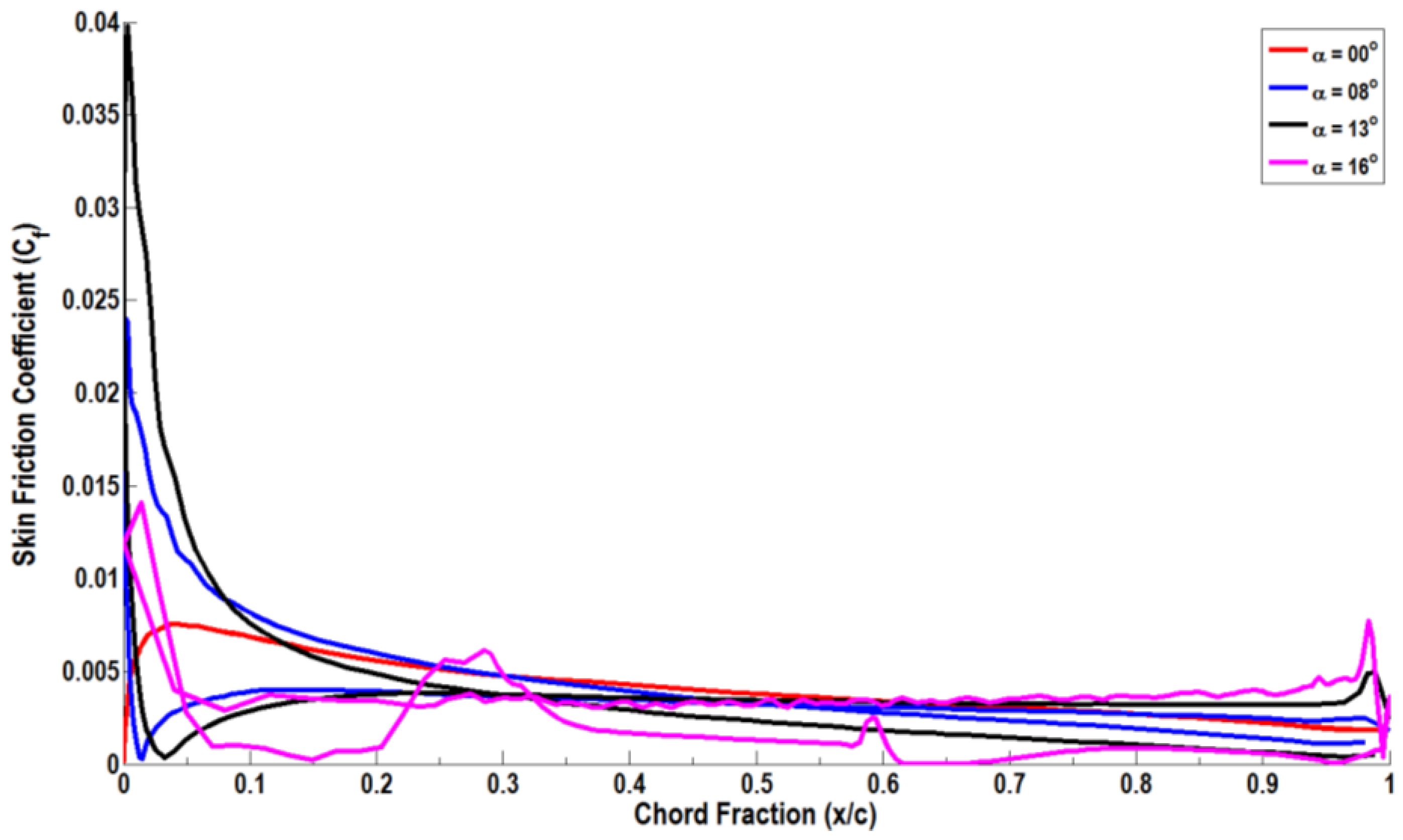
For better understanding of the airflow characteristics around the airfoil, variations of the skin friction coefficient are evaluated for selected incidence angles, as shown in
Figure 9. The skin friction coefficients increase with the incident angle and also show a smooth variation for angles of attack equal to or smaller than 13°. The skin friction coefficient curve at α = 16° shows an irregular variation, which is a typical trend for the cases when there are some separation zones.
Figure 10 shows the variation of the lift coefficient with the incidence angle at free stream conditions corresponding to a chord Reynolds number of 10
6. The lift and drag coefficients from the ANSYS-Fluent RANS simulations were calculated, and the results for the lift coefficient are shown in this figure. It is seen that the lift coefficient increases with the angle of attack up to about 13° and then decreases. The lift coefficient obtained from 2D potential flow analysis using the panel method, the RANS simulation results of Joslin et al. [
29] and the large eddy simulation results of You and Moin [
2] are also shown in this figure for comparison. In addition, the experimental data of Rethmel [
27] for the NACA 0015 at chord Re = 10
6 and the data of Lasse and Niels [
30] at a chord Re of 1.6 × 10
6 are also reproduced in
Figure 10. It should be pointed out that the potential flow solution that treats the flow around the airfoil as inviscid and irrotational is an idealized case for extremely high Reynolds number flows [
31].
It is seen that the lift coefficient increases with the incidence angle up to α = 13°, after which lift starts to decrease. The present RANS-realizable
k-ε turbulence model simulation results are in general agreement up to the point of separation with earlier RANS results of Joslin et al. [
29], Large Eddy Simulation (LES) results of You and Moin [
2] and the experimental data of Rethmel [
27] and Lasse and Niels [
30]. After the point of separation, the current RANS predictions are in general agreement with the experimental data of Rethmel [
27], as well as the LES results of You and Moin [
2]. The RANS simulations of Joslin et al. [
29] that use the one-equation Spalart–Allmaras turbulence model, however, over-predict the LES and the experimental data.
While the present RANS simulations for the lift coefficient are in good agreement with the experimental data of Rethmel [
27], the matching of the integrated lift coefficients does not necessarily ensure agreement in the pressure distribution around the airfoil.
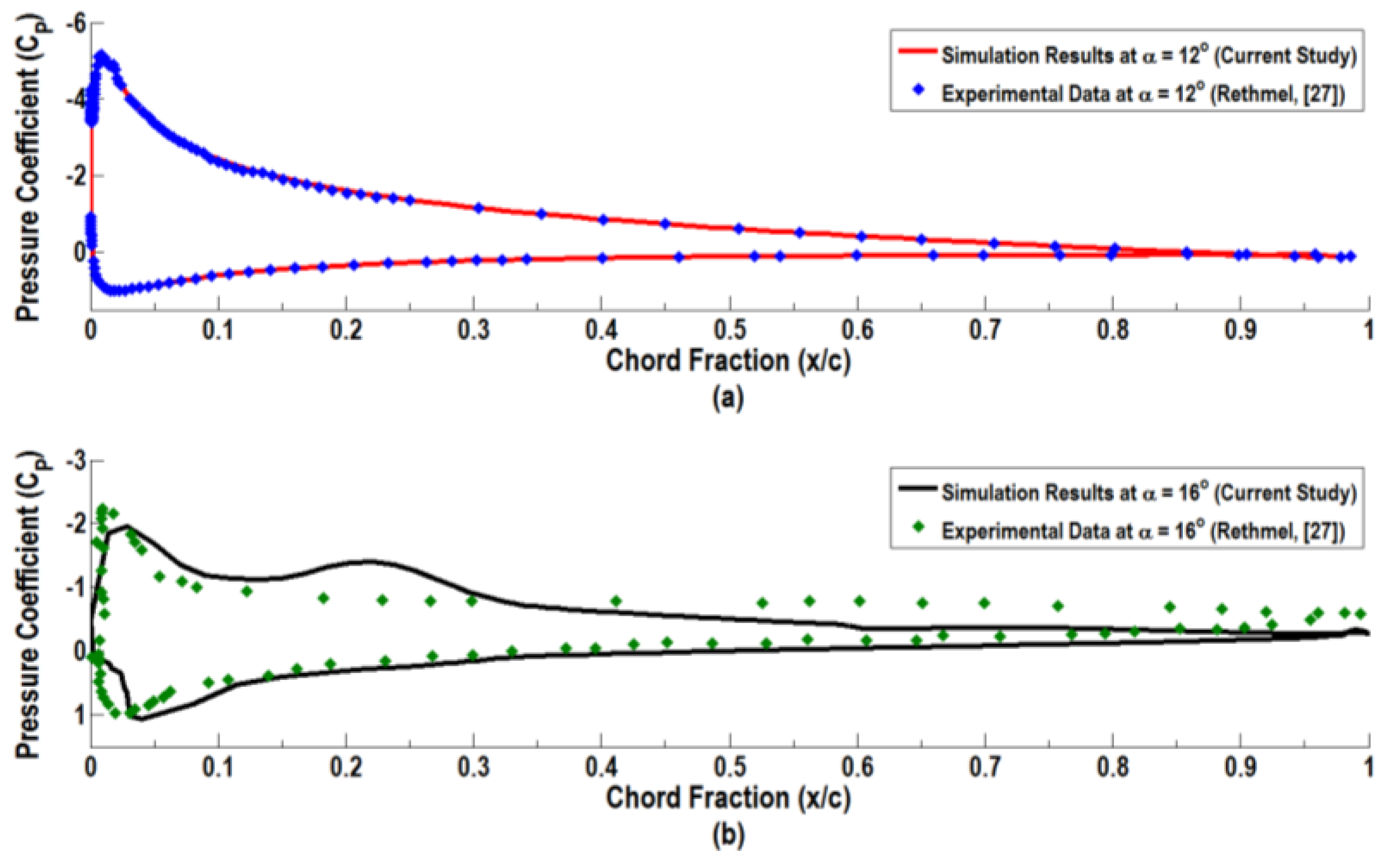
Figure 11a shows the chord-wise distribution of pressure coefficient
Cp on the airfoil as predicted by the present RANS simulation at the onset of stall (α = 12°). The experimental data of Rethmel [
27] are reproduced in this figure for comparison. Excellent agreement in the chord-wise distributions of the predicted pressure coefficient with the experimental data is seen from this figure. This emphasizes the observation that the realizable
k-ε turbulence model provides an accurate description of the pressure distribution around the airfoil at this incidence angle.
For angles of incidence in the stalled regime (α > 13°), the flow separation occurs, and the accuracy of the realizable
k-ε turbulence model in predicting the separated flow structures becomes somewhat questionable. In fact, a careful examination of
Figure 10 reveals that the
k-ε turbulence model slightly over-predicts the experimental lift coefficient at high angles of attack of α = 13°–14°. To examine this trend,
Figure 11b shows the distribution of
Cp as predicted from the current RANS simulation at the fully-developed stall regime (α = 16°) and compares them with the experimental data of Rethmel [
27]. There are noticeable differences between these pressure distributions.
It is worth mentioning that the maximum lift coefficient predicted by the present simulations is 1.15 for α = 13°. The slope of the lift curve obtained from the current study, as well as those for the earlier numerical results and experimental data is for low AoA, which remains constant for incidence angles up to about 11°. The slope of the lift curve is for the potential flow case.
Figure 12 exhibits the predicted variation of drag coefficients with the incidence angles and provides comparison with the earlier RANS simulations and the experimental data. As expected, the drag coefficient increases with the increase of incidence angle. The RANS simulation results of Schroeder [
32] for the NACA 0012 airfoil at Re = 10
6 and the drag coefficient measurements’ data of Sharma [
33] for the NACA 0015 at Re = 0.7 × 10
6 are reproduced in this figure for comparison. In addition, the drag coefficient data of Sheldahl and Klimas [
34] for the NACA 0015 at Re = 10
6 and those of Lasse and Niels [
30] at Re = 1.6 × 10
6 are also shown in this figure. It is seen that the drag coefficient values predicted by the realizable
k-ε model are in reasonable agreement with the experimental data and earlier numerical results for incident angle less than 13°. The drag coefficient is low at zero incidence angles and increases slowly with the angle of attack to the value of 0.038 at the stall condition. The slope of the drag coefficient with respect to incidence angle,
remains roughly constant at about 0.003. After the stall condition, the drag coefficient increases rapidly with the further increase of the angle of attack and reaches a value of 0.28 at α = 20°, which is more than seven-times the drag coefficient at the stall condition. The slope of the drag coefficient versus incidence angle,
, jumps to a value of 0.04 after the stall condition. It is also seen that the value of the drag coefficient decreases with the increase of the Reynolds number. It is also observed that for an incident angle beyond separation, the present model overestimates the experimental data for the drag coefficient. Further study of the accuracy of various turbulence models including the realizable
k-ε turbulence model are left for a future work.
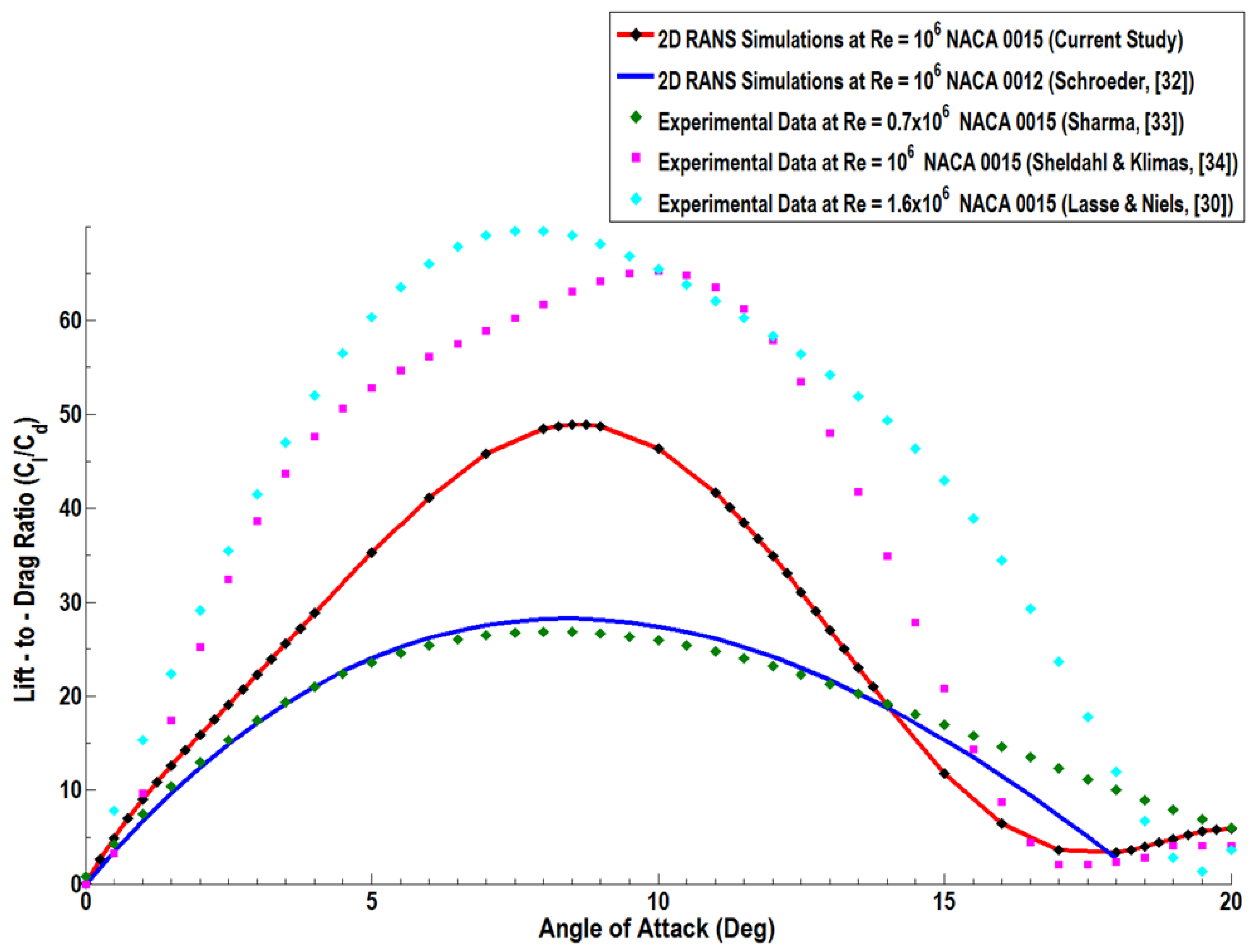
Figure 13 shows the variation of the lift-to-drag ratio
/
) with the incidence angle as predicted by the realizable
k-ε model and the comparison with the available experimental data and earlier simulations. It is seen that the lift-to-drag ratio increases rapidly from zero at α = 0° toward its maximum value with the increase in incidence angle. This is because for small angles of attack, both
and
increase, but
increases faster than
[
35]. Then, as the angle of attack further increases, the lift-to-drag ratio decreases, and the decreasing trends are continuous to beyond the stall angle.
While the trend of variations of the lift-to-drag ratio of the present simulations is in qualitative agreement with the experimental data and earlier simulations, there are quantitative differences in the peak value of this ratio. The maximum value of lift-to-drag ratio found for the present simulations is 48.2, which occurs at AoA of 8.5°.
Figure 13 shows that the maximum value of lift-to-drag ratio for most cases occurs at AoA of 8°–8.5°, except for the data of Sheldahl and Klimas [
34], for which the peak occurs at AoA of 10°. This figure also shows that the lift-to-drag ratio could reach a peak value of about 65.
Another result obtained from this study is the behavior of the turbulence intensity of the flow around the airfoil. Here, the turbulence intensity (TI) is defined as the ratio of root mean square velocity fluctuation
, to the mean local flow velocity
(Fluent lecture notes [
23]).
Figure 14 shows the turbulence intensity contours around the airfoil for selected incidence angles as a percentage. It is seen that the turbulence level increases with incident angle and could reach a maximum of 49% for the range of incidence angles considered. At zero incidence angle, the maximum turbulence intensity occurs near the leading edge of the airfoil. At an incidence angle of 5°, the contour map of turbulence intensity shows a slight shift of the location of the maximum intensity region toward the trailing edge on the upper surface of the airfoil.
Figure 14 also indicates that at low incidence angles up to about 12°, a turbulent boundary layer is attached to the airfoil, and only a thin wake is formed behind the airfoil. When the airfoil incidence angle is increased to 13° or larger (where the flow separation is expected to occur), the wake becomes much larger, and the region with maximum turbulent intensity becomes larger and departs further from the airfoil surface. For the airfoil incidence angle of 20°, the airfoil is passing through a deep stall, where the airflow on its upper surface separates right after the leading edge and produces a wide wake. In this case, the maximum turbulence intensity region occupies a large zone off the airfoil surface, but close to the trailing edge.
Table 6 lists the predicted maximum turbulence intensities as a percent for several incidence angles. The simulation results of Zhang et al. [
17] for airflow around the NACA 0015, who used the
k-ω model at Re= 0.55 × 10
6, are also reproduced in this table for comparison. It is seen that the results of the present realizable
k-ε model for the peak turbulence intensity are in qualitative agreement with those reported by Zhang et al. [
17].
Table 6 also shows the expected increasing trend of turbulence intensity with the angle of incidence.
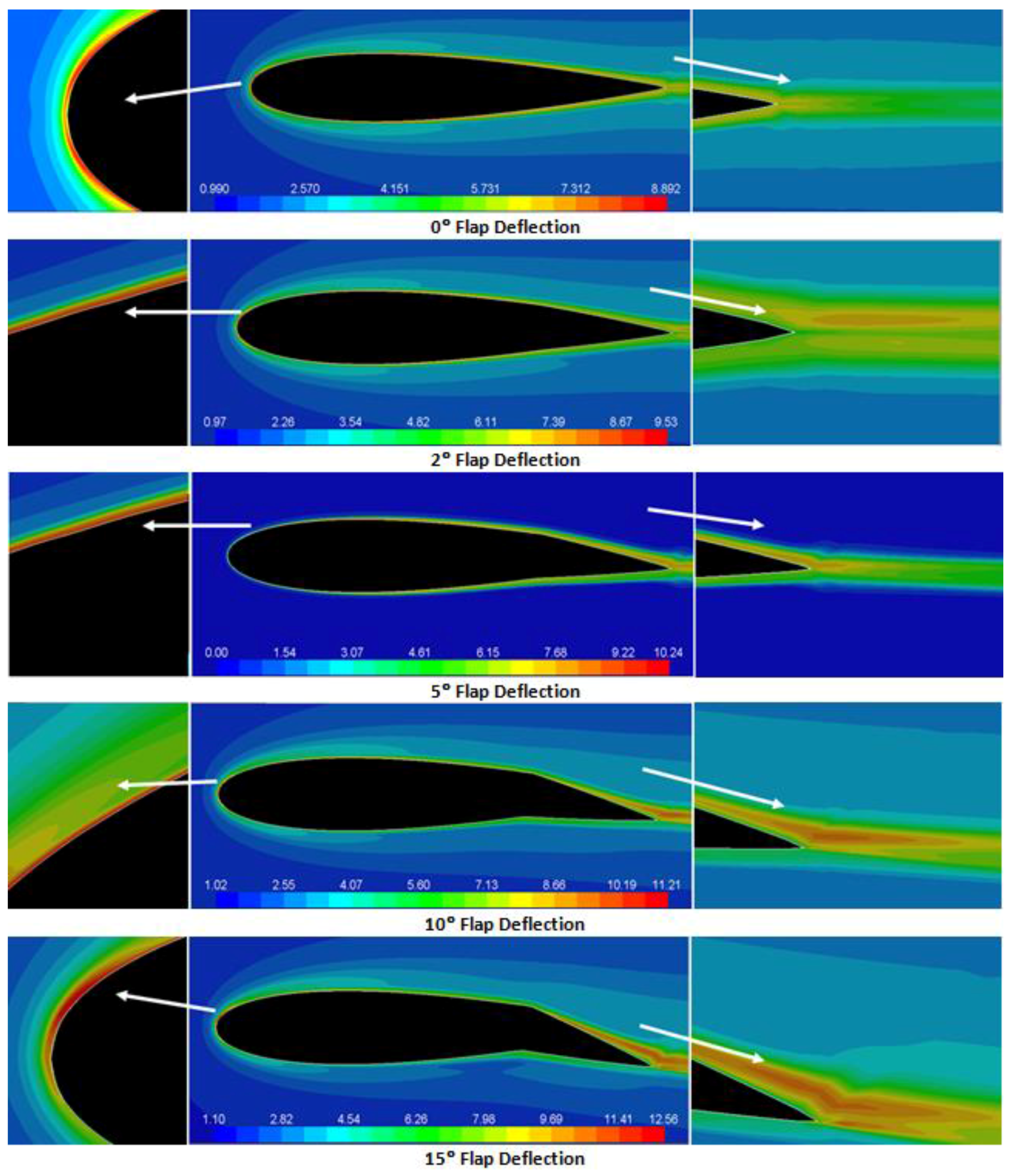
3.3. NACA 0015 Airfoil with Flap Deflection
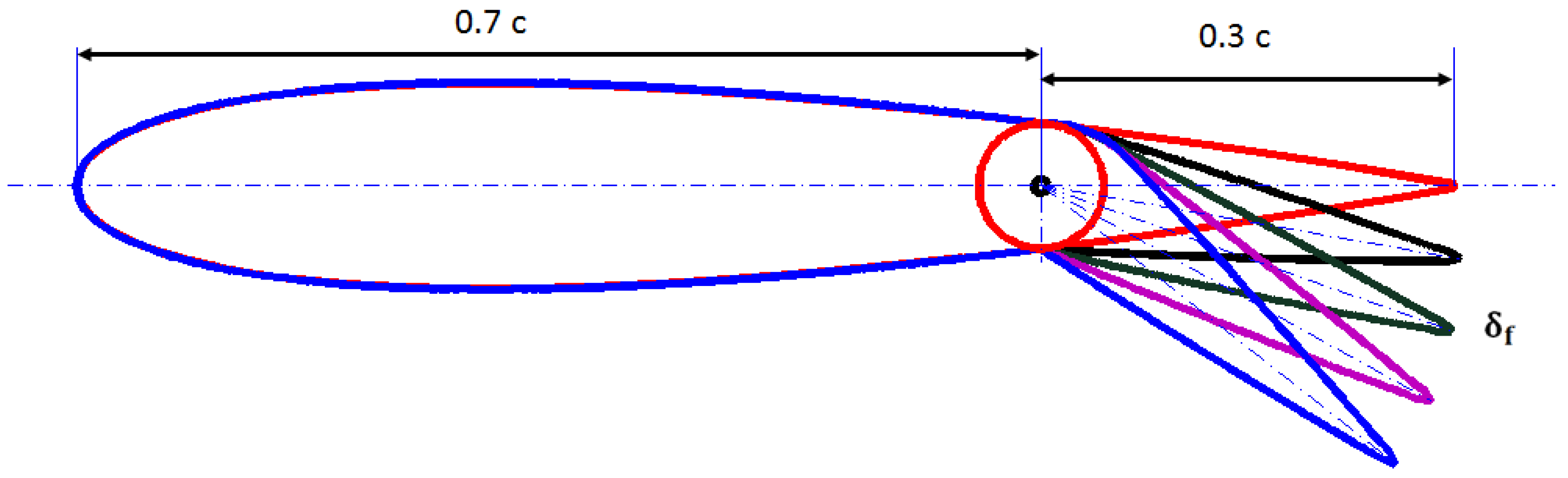
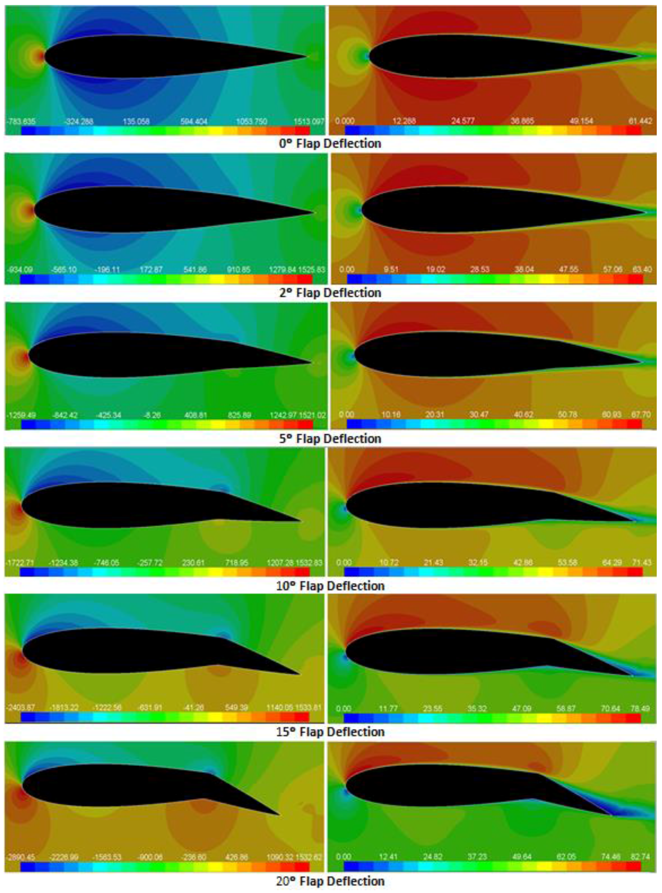
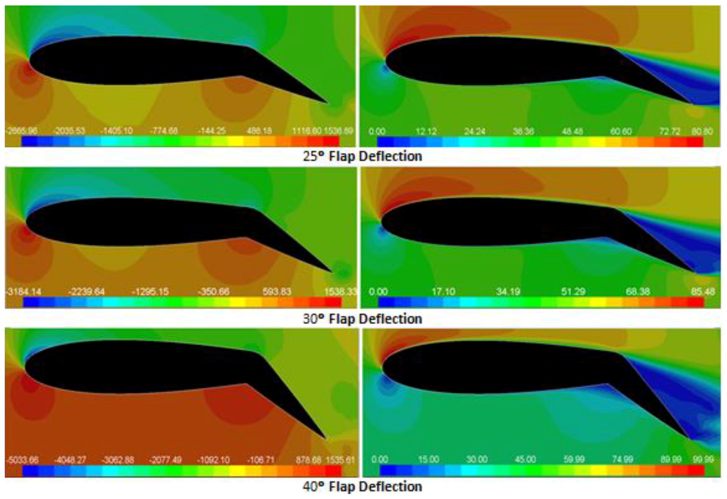
The effect of downward flap deflection on the aerodynamic performance of the airfoil is studied for eight different flap positions of 2°, 5°, 10°, 15°, 20°, 25°, 30° and 40°. For zero AoA, the static pressure and velocity contours for different flap deflections (δ
f) are presented in
Figure 15. The comparison of the static pressure contours for zero flap deflection and for the deflected flap at the same angle of attack shows that the flap deflection increases the negative pressure over the entire upper surface of the main airfoil and increases the positive pressure on the lower surface near the trailing edge. The pressure on the lower surface increases rapidly with flap deflection, while the pressure on the upper surface increases gradually. The pressures on both the upper and the lower surfaces of the flap increase with flap deflection.
One other interesting observation is the progressive increase of the velocity magnitude over the upper surface of the main airfoil as the flap deflection increases. The flap deflection changes the velocity and pressure distributions on the airfoil upper and lower surfaces, causing higher pressure to be built over the rear portion, generating a net lift force at AoA = 0°, and increases the airfoil maximum lift coefficient. The flap deflection also moves the zero lift angle-of-attack of the airfoil to a lower negative value and greatly increases the drag force.
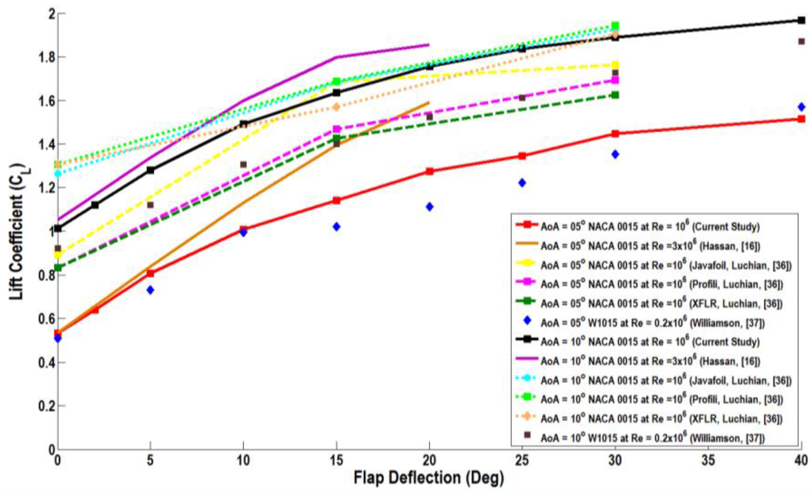
Figure 16 shows the predicted variation of the lift coefficient with the flap deflection at two different angles of attack of α = 5° and α = 10°. Here, the realizable
k-ε predictions are compared with the simulation results of Hassan [
16] and Luchian [
36], as well as the experimental data of Williamson [
37]. Hassan [
16] studied the aerodynamic performance of the NACA 0015 airfoil with a 25% trailing edge flap at Re = 3 × 10
6 and for different Mach numbers. Luchian [
36] investigated the aerodynamic performance of the NACA 0015 airfoil with a 27.5% trailing edge plain flap for different flap deflection angles at Re = 10
6 by using three different codes (Javafoil 2.20, Martin Hepperle, Braunschweig, Germany, Profili2.20, Stefano Duranti, Feltre, Italy, and XFLR5 6.06, techwinder, Paris, France). Williamson [
37] conducted experiments on the W1015 airfoil, which is identical to the NACA 0015 airfoil for wide range of low Reynolds numbers and trailing edge flap deflections. It is evident that the lift coefficient increases sharply with the increase of the flap deflection up to about 10°–15°, and then, the rate of increase becomes slower up to δ
f = 40°. The present model predictions are in general agreement with the results of Hassan [
16] for high Reynolds numbers for flap deflections up to δ
f = 20°, the results of Luchian [
36] at low Reynold numbers for flap deflections up to δ
f = 30° and the experimental data of Williamson [
37] for low Reynolds numbers for a wide range of flap deflections up to δ
f = 40°.
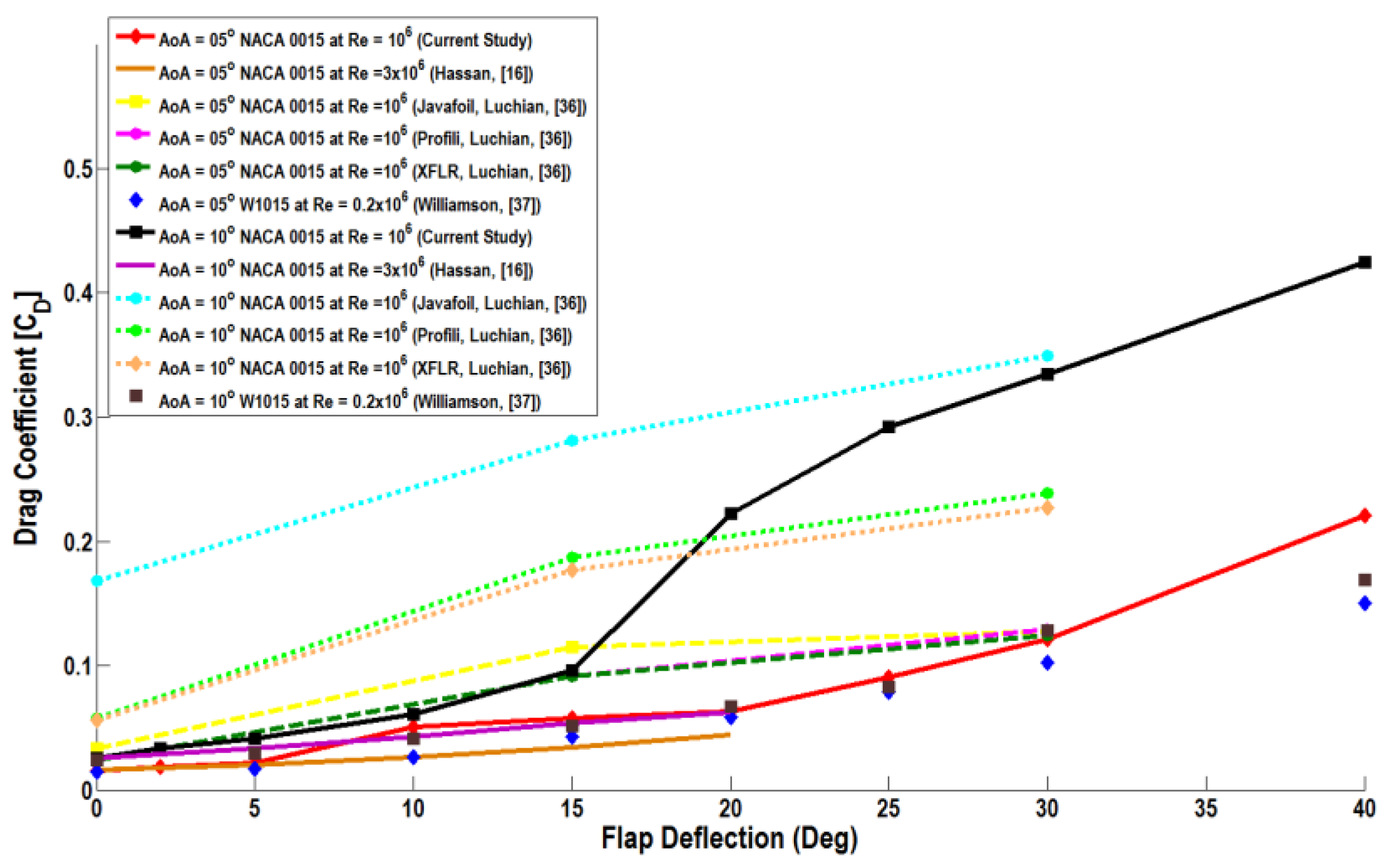
Figure 17 shows the predicted variation of the drag coefficient with the flap deflection at two different angles of attack of α = 5° and α = 10°. For α = 5°, the drag coefficient of the flapped airfoil increases gradually with the flap deflection up to a flap angle of δ
f = 20°, and then, the rate of increase becomes much shaper. For example, the drag coefficient at δ
f = 30° is more than two-times its value at δ
f = 15°. The trend is somewhat different for the AoA of α = 10°, where the drag coefficient increases gradually with the flap deflection up to δ
f = 15°, and then, the drag coefficient increases sharply. The drag coefficient for δ
f = 30° in this case is more than five-times its value at (δ
f = 10°). When compared with the earlier results, the drag coefficients obtained by the realizable
k-ε model in this study are reasonably accurate for the AoA = 5° and in the entire range of flap deflections up to δ
f = 30°. It is clear that for the AoA = 10° and δ
f > 15°, the predicted drag values are somewhat higher than those predicted by both the Profili and XFLR5 codes, but below the values obtained by the Javafoil code.
The effect of flap deflection on lift increment is presented next. A lift increment
is the amount of lift that is gained or lost due to a flap deflection measured from a reference configuration. The airfoil with zero flap deflection is taken as the reference case. The trend in these plots is compared with the experimental data of Williamson [
37] for the W1015 symmetrical airfoil tested at Re = 4 × 10
5 at zero flap deflection and 10° flap deflection.
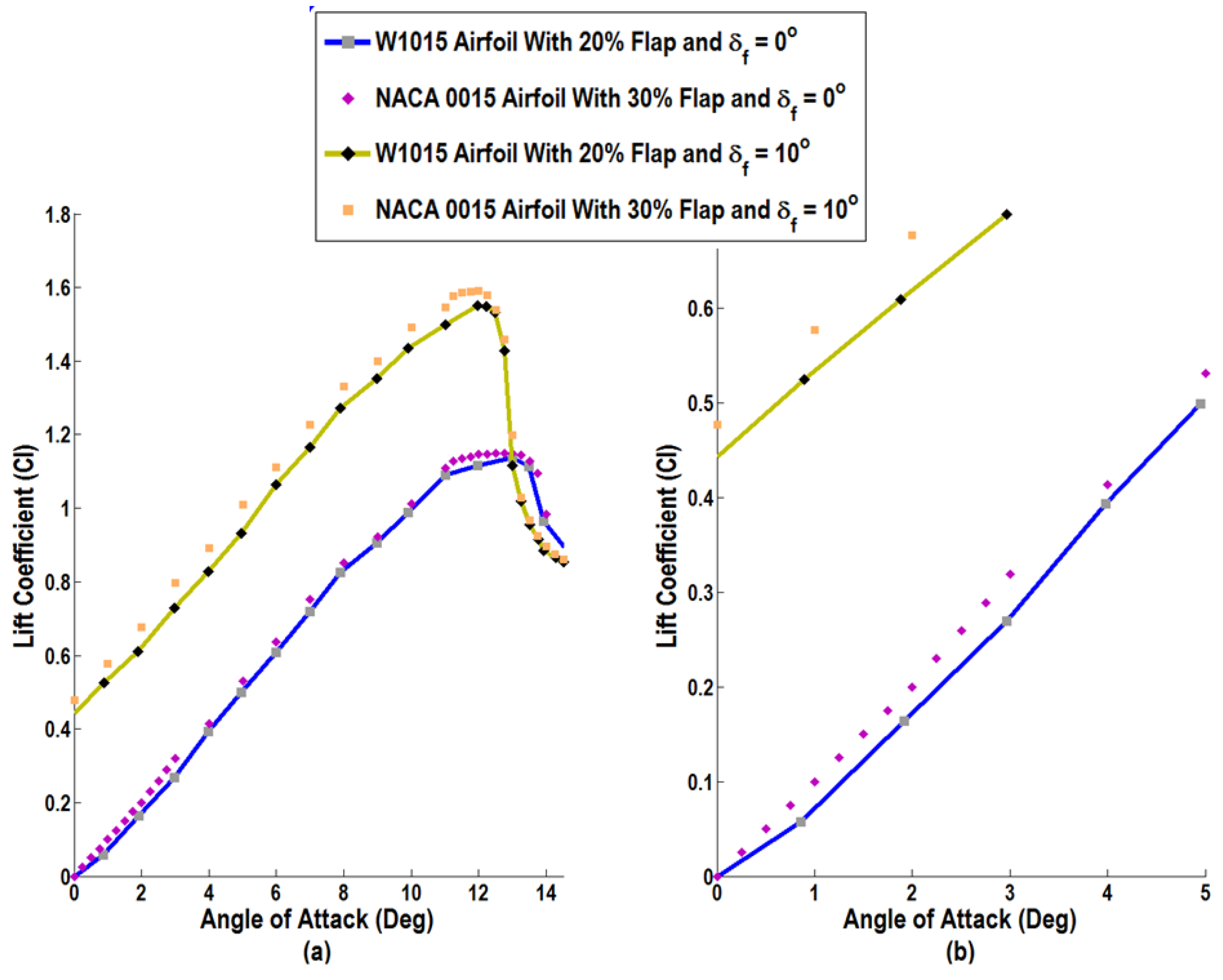
Figure 18a exhibits the variation of the lift coefficient with the angle of attack at a flap deflection of δ
f = 10° together with their corresponding reference values at δ
f = 0°.
Figure 18b presents an enlarged section of the lift coefficient for small angles of attack. In addition, the increments in the values of the lift coefficient are shown in
Figure 18b. It is seen that the lift increment value
due to the flap angle is roughly the same for a large range of incidence angles below the stall angle. That is,
for the airfoils with zero and 10° flap angle.
In
Figure 18b, it can be seen that at δ
f = 0°, the slope of the lift curve for the W1015 airfoil is slightly lower than the slope of the lift curve for the NACA 0015. It should also be pointed out that the W1015 airfoil was tested at Re = 4 × 10
5, and the NACA 0015 results are for Re = 10
6. It is also known that for the same angle of attack, a higher Reynolds number gives higher lift coefficient and consequently a greater slope of the lift curve. The lift curves for both airfoils are nearly linear at low angles of attack (below 10°).
Due to the flap deflection, it is observed that the lift coefficient has a nonzero value at zero AoA for both airfoils. For both airfoils, the lift increment is nearly constant at low angles of attack. The lift increment is slightly higher for the NACA 0015 due to the higher Reynolds number for the flow computations.
Table 7 shows the values of the increments in the lift coefficient obtained due to a flap deflection of 10° for both airfoils.
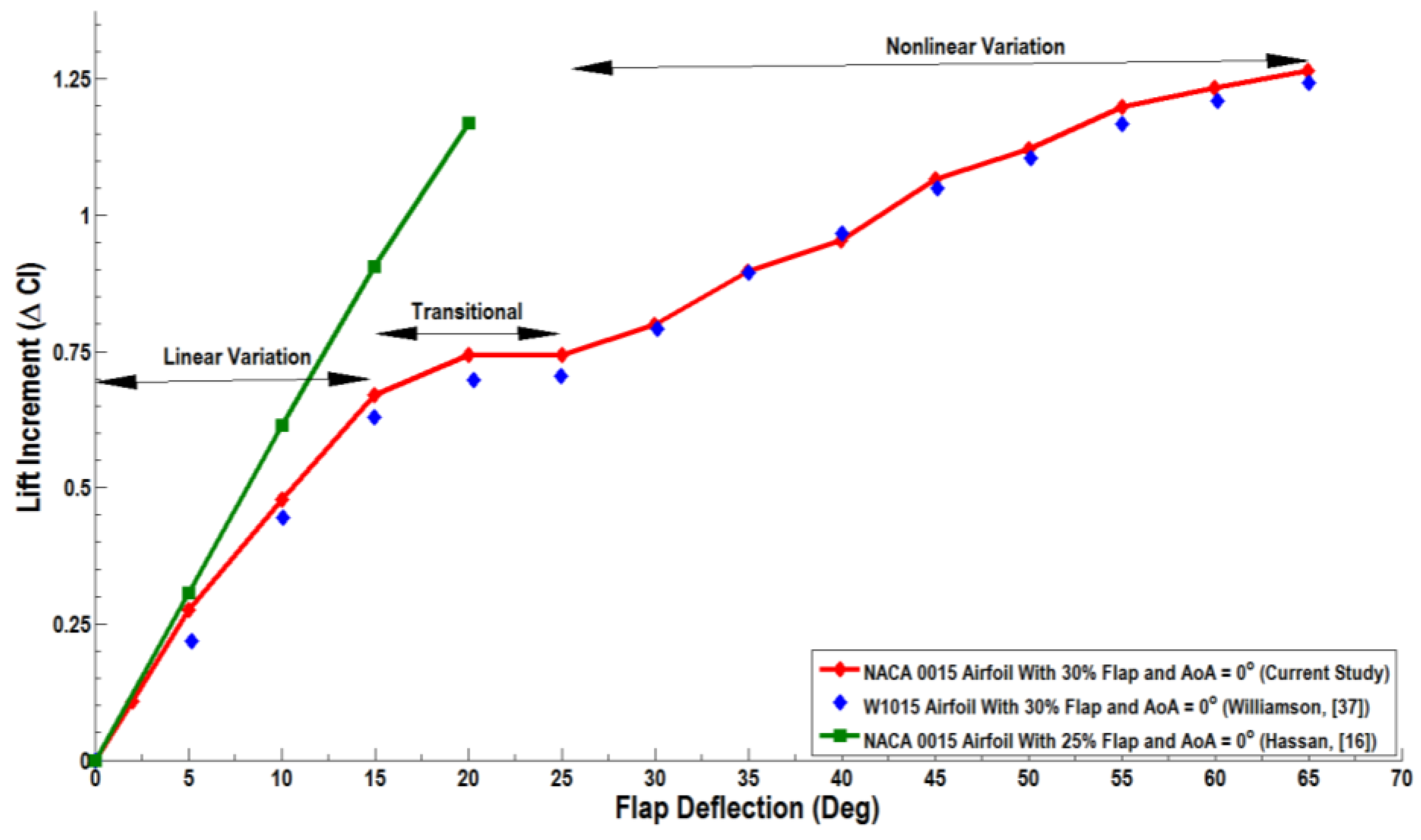
Simulation results for the lift increment due to flap deflection at zero angle of attack for a wide range of flap deflections are plotted in
Figure 19, and the results are compared with the experimental data. There are three distinct regions that define different trends of
∆Cl values. A linear region is observed at smaller flap deflections of 0 ≤ δ
f ≤ 15°. In this region, the slope of the
ΔCl curve is constant, indicating fully-attached flow conditions. The second region is the transitional region, as it acts as a connection between linear and nonlinear regions. It is normally marked as the leveling or decreasing of
ΔCl values that is caused by the separation of flow from the upper surface of the flap. Separation from the upper surface normally occurs around a flap deflection of 10–20 deg. The actual flap deflection for flow separation depends on the Reynolds number, airfoil thickness, flap-chord ratio, angle of attack and the size of the gap around the nose of the flap. The third region is nonlinear in nature due to the reduced nonlinear increase of
ΔCl values with flap deflection. In this region, the flow is largely separated over the upper surface of the flap.
Figure 19 shows that the current realizable
k-ε model predictions for the lift increment are in close agreement with the experimental data of Williamson [
37]. For flap deflection angles δ
f ≤ 20°, it is seen that the lift increment
ΔCl varies linearly in the simulations. The simulations of Hassan [
16] were for a high Reynolds number flow and have a linear trend, but a higher slope. For high flap deflections (δ
f > 20°) and a high Reynolds number, Hassan [
16] did not provide any data. From
Figure 19, it is concluded that the present model predictions are reasonably accurate at least for low Reynolds number flows.
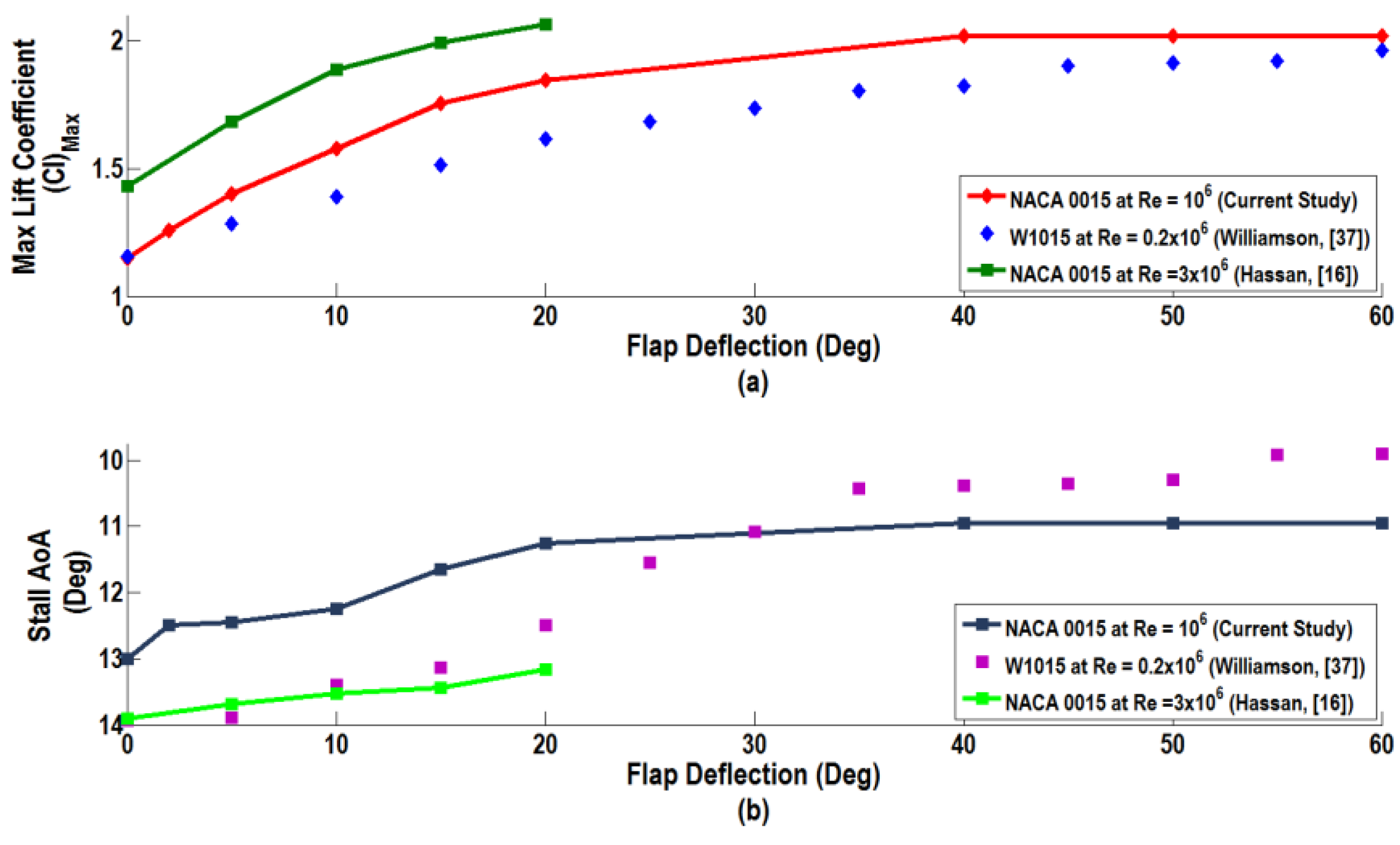
It is of interest to study the effect of the flap deflection on both the maximum lift coefficient and the corresponding angle of attack (critical or stall AoA). The variation of the predicted maximum lift coefficient versus flap deflection is shown in
Figure 20a, while the variation of the stall angle of attack is illustrated in
Figure 20b. In these figures, the corresponding results of Williamson [
37] and Hassan [
16] are reproduced for comparison.
Figure 20a shows that the maximum lift coefficient increases linearly for small flap deflections 0 ≤ δ
f ≤ 15°. For flap deflections larger than 15°, however, the increasing slope of the maximum lift coefficient is reduced and reaches a plateau for the flap deflection in the range of 40° < δ
f < 60°. Thus, it can be concluded that deflection of the flap δ
f > 40° does not provide additional benefit in regard to the maximum lift coefficient.
Figure 19a also shows that the trends of the maximum lift coefficient obtained by the present realizable
k-ε model are comparable to those of the experimental data of Williamson [
37] for the W1015 airfoil, as well as the results of Hassan [
16] for the NACA 0015 airfoil. The magnitudes are, however, somewhat different, and the present simulation results lie in between the results of Williamson [
37] and Hassan [
16].
Figure 20b shows the variation of the stall angle versus flap angle. It is seen that the current model predictions follow the general trend of the published results, as the stall angle of attack at which
Cl, max is achieved decreases with increasing the flap deflection. Deflecting the flap by 20° decreases the stall angle of attack by 1.75° in the present study, while leading to a decrease of 1.5° in the experimental study of Williamson [
37] and 0.75° in the results of Hassan [
16]. The further increase in the flap deflection decreases the stall angle of attack. The present model predicts that lowering the flap by 40° decreases the stall angle of attack by 2°, while Williamson’s [
37] data suggest a decrease of the stall angle of attack by 4°.
The turbulence intensity contours of the flow around the flapped airfoil at some selected deflection angles and zero incidence are also evaluated.
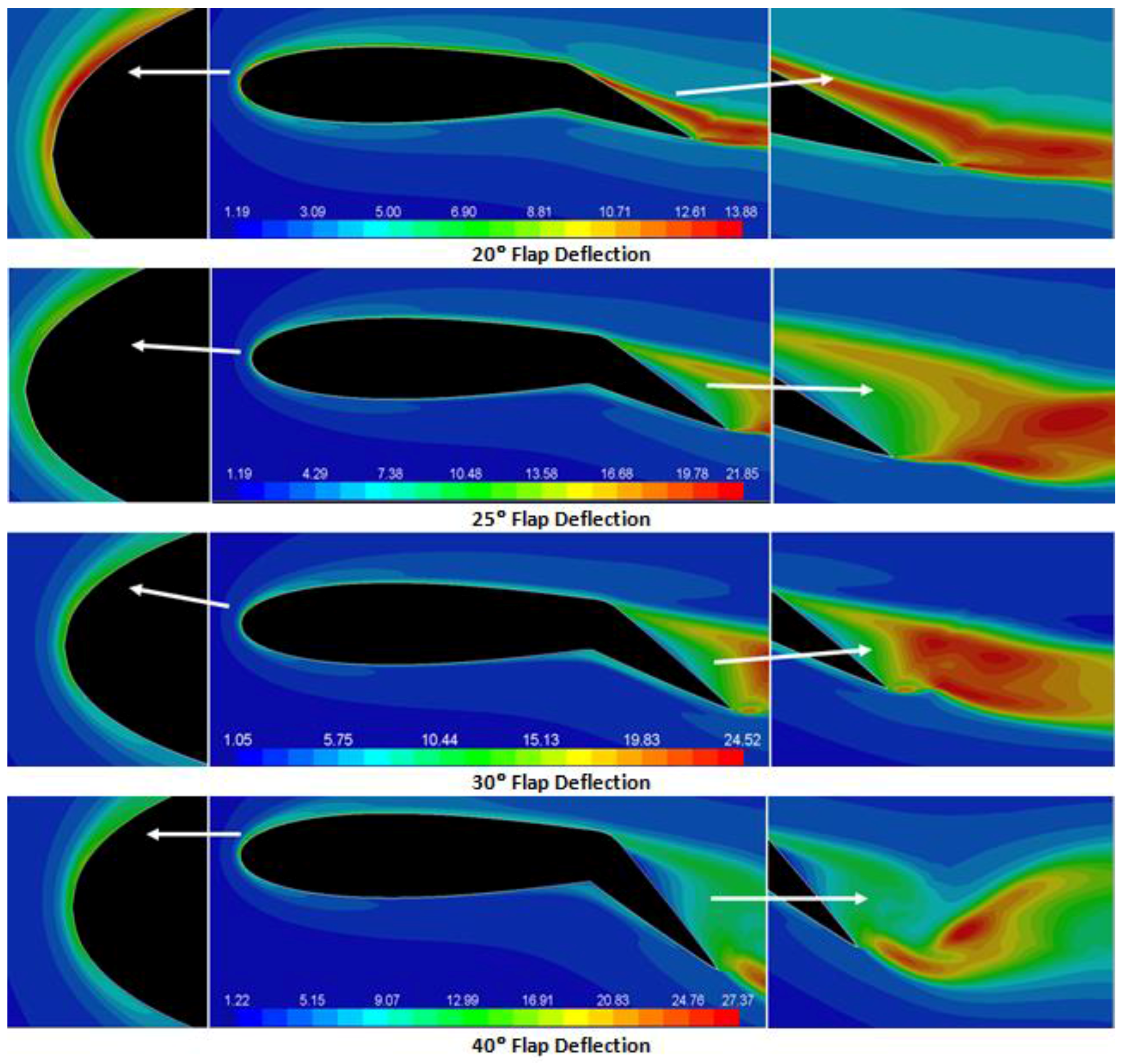
Figure 21 presents the contours of turbulence intensity at δ
f 2°, 5°, 10°, 15°, 20°, 25°, 30° and 40° and for zero incidence angle. It is observed that at the zero incidence angle, the flap deflection has a pronounced influence on the turbulence intensity around the flapped airfoil. Even a small deflection in flap angle disturbs the flow and creates regions of high turbulence intensity in the upper surface of the flapped airfoil. These regions expand with increasing of the flap deflection and shift from the main airfoil towards the flap section. For δ
f ≤ 15°, the realizable
k-ε model predicts that the peak turbulence intensity occurs in the boundary layer near both the upper and lower surfaces of the main airfoil close to the leading edge and with a lower level of turbulence intensity in the wake region. For δ
f ≥ 15°, however, the maximum turbulence intensity occurs in the wake region close to the flap in addition to the boundary layer regions. This is due to the fact that the region with recirculating flow becomes larger as the wake width increases with the flap deflection. At high flap deflections, the flow separates from the flap, and high pressure acting on the pressure side of the flapped airfoil and consequently marked increase in the drag occur compared to situations where the flow remains attach to the surface.


