
Hydrodynamics of Highly Viscous Flow past a Compound Particle: Analytical Solution

Department of Mathematics, Applied Mathematics and Statistics, Case Western Reserve University, Cleveland, OH 44106, USA
Fluids 2016, 1(4), 36; https://doi.org/10.3390/fluids1040036
Submission received: 23 September 2016
/
Revised: 6 November 2016
/
Accepted: 7 November 2016
/
Published: 12 November 2016
(This article belongs to the Special Issue Mechanics of Fluid-Particles Systems and Fluid-Solid Interactions)
Abstract
:To investigate the translation of a compound particle in a highly viscous, incompressible fluid, we carry out an analytic study on flow past a fixed spherical compound particle. The spherical object is considered to have a rigid kernel covered with a fluid coating. The fluid within the coating has a different viscosity from that of the surrounding fluid and is immiscible with the surrounding fluid. The inertia effect is negligible for flows both inside the coating and outside the object. Thus, flows are in the Stokes regime. Taking advantage of the symmetry properties, we reduce the problem in two dimensions and derive the explicit formulae of the stream function in the polar coordinates. The no-slip boundary condition for the rigid kernel and the no interfacial mass transfer and force equilibrium conditions at fluid interfaces are considered. Two extreme cases: the uniform flow past a sphere and the uniform flow past a fluid drop, are reviewed. Then, for the fluid coating the spherical object, we derive the stream functions and investigate the flow field by the contour plots of stream functions. Contours of stream functions show circulation within the fluid coating. Additionally, we compare the drag and the terminal velocity of the object with a rigid sphere or a fluid droplet. Moreover, the extended results regarding the analytical solution for a compound particle with a rigid kernel and multiple layers of fluid coating are reported.
1. Introduction
The flow around an object moving in highly viscous, impressible fluid has been an interesting subject in fundamental studies and applications. The applications range widely from the determination of electron charges [1,2,3], physics aerosols [4], and medical applications [5], to biotechnological industries and engineering processes. From the very first study on the effects of viscosity pendulums [6], to a rigid body moving in an arbitrary flow [7], to fluid drops translating in another fluid [8], numerous works considering the motion of rigid and fluid objects in both bounded and unbounded domains have been reported. In the body frame, the translation of a particle in fluid is equivalent to the flow past a fixed obstacle. The problem of Stokes flow past a spherical object is an important one, owing to the manifold applications in science and engineering.
To analyze the flows, explicit and analytical solutions play a critical role. For example, an analytical solution is the starting point of the stability of a particle sediment. However, analytical solutions are rarely obtained for objects moving in flows, even in the Stokes regime. Uniform flow past a rigid sphere is first extensively studied [9], then the study of exact solutions is extended to the linear flow past an ellipsoid [10], and more work about other background flows past spheres or a spheroid [11]. Utilized with a singularity method, studies have been extended to linear and quadratic flow past a spheroid [12,13,14,15]. The exact solution of uniform flow past a fluid drop has also been reported [16,17].
Recently, compound multiphase particles have received much interest because of their significance in a variety of biomedical applications [18,19,20,21,22,23]. Johnson [19] studied the uniform Stokes flow past a rigid sphere with a thin immiscible fluid film covering its surface using a perturbation scheme. In his work, the fluid-film profile is achieved by numerical calculations. Later, Johnson and his collaborators further studied bubbles and drops partially coated with thin films [24,25]. Gupta et al. [26] extended Johnson’s work [19] to micropolar fluid for the outer region [26]. Rushton and Davies [27] studied an encapsulated droplet, which is a spherical two-layer fluid object. However, they focused on the drag force only. In their paper, there is no report about parameters for the stream functions, which are keys to exploring the flow pattern. Also, it is important to notice that the boundary conditions at the interface inside the fluid drop are different from the boundary conditions between the rigid kernel and the fluid coating of the object studied in this paper. Li and Pozrikidis [28], and Blawzdziewicz et al. [29] investigated the effects of insoluble surfactants on the hydrodynamics and rheology of dilute emulsions in Stokes flow numerically. Most recently, Datta and Raturi [30] studied a swarm of spherical particles by modifying boundary conditions to account for the interaction effect. However, the flow with compound particles is not fully understood yet.
In this paper, we study the problem of a rigid spherical kernel, with a fluid coating, falling freely in a viscous dominated fluid. In the body frame (the moving frame), this is the problem for uniform flow past a fixed spherical object. Rigorous analytical solutions for stream functions are achieved by taking advantage of the axial symmetry properties. The hydrodynamic drag and terminal velocity are analyzed. From a rigid kernel with one layer of fluid coating, we extend the study to spherical particles with multiple-layer coating. Results from this study can shed light on the hydrodynamics of biomedical applications with similar obstacles. In those applications, the movement of particles is essential for drug delivery [31,32] and metastasis movements [33] of cancers. For example, magnetic beads coated with antibodies are used to isolate circulating tumor cells [34].
2. Formulation of Problem
Assume that a sphere with a rigid kernel and a fluid coating is embedded in unbounded, uniform fluid flow with constant velocity , density ρ and dynamic viscosity μ. The rigid kernel
is covered by a layer of fluid coating. The fluid coating with thickness occupies
Figure 1 schematically illustrates the setup of the problem.
If the thickness of the fluid layer, d, is zero, this is reduced to the problem of uniform flow past a purely rigid sphere. If the radius of the rigid kernel, a, is zero, the problem is indeed the flow past a fluid drop, as long as . The density and dynamic viscosity of the fluid within the layer of coating are and , respectively. The fluid in the coating is assumed to be immiscible with the surrounding background fluid and the surface tension at the fluid interface is sufficiently strong to keep the obstacle spherical against any deformation.
Since both fluids are incompressible, the continuity equation is where is the flow velocity. In this paper, we assume that the inertial terms in the Navier–Stokes equations for both fluids can be neglected. Thus, the equations of motion are
where p denotes the fluid pressure. Similar governing equations apply to the fluid coating, but the viscosity of the fluid can be different from the viscosity μ of the fluid in the unbounded domain. Later, subindices are also used to identify different fluids. The condition for (3) to hold is that , where U is the magnitude of the uniform velocity . For example, the Reynolds number is about ∼ for the flow with / past a Xenopus oocyte [32,35]. The boundary conditions are no-slip boundary condition at the solid–fluid interface, and no-slip and no interfacial mass transfer condition (no penetration and continuity of tangential velocity) at the fluid interface. This forms a force equilibrium condition at the fluid–fluid interface. Also, is asymptotic to the basic uniform flow at large distances from the obstacle. These conditions are specified explicitly when we derive analytical solutions.
3. Analytical Solution for Uniform Flow past Spherical Objects
Before reporting the solution for the uniform flow past a general two-layer obstacle at Section 3.3, two extreme cases are reviewed. The case is the well-known result for a uniform flow past a fixed rigid sphere. The other one is the flow past a fluid drop, in which the viscosity is different from the background flow. The two fluids are immiscible. These simple cases are documented in the paper to make it self-contained when we compare the results between different problems. As we provide the results for these simple cases, it is also helpful to illustrate the derivation of the general multiple-layer obstacle.
3.1. Uniform Flow past a Rigid Sphere
If the thickness d of the fluid coating is zero in Figure 1, this is the well-known uniform flow past a rigid sphere. With the axisymmetric property, the problem is reduced to two dimensions. In this situation, the stream function and velocity can be found in the literature. In spherical polar coordinates ( in the direction of ) the stream function is [16,17,36]
This result was obtained by Stokes [6]. Inside the parentheses, the first term corresponds to the uniform background flow, and the second term is due to the doublet [12]; together they represent an inviscid flow past a sphere. The third term representing the viscous correction is the Stokeslet. The velocity components and in the polar coordinates are
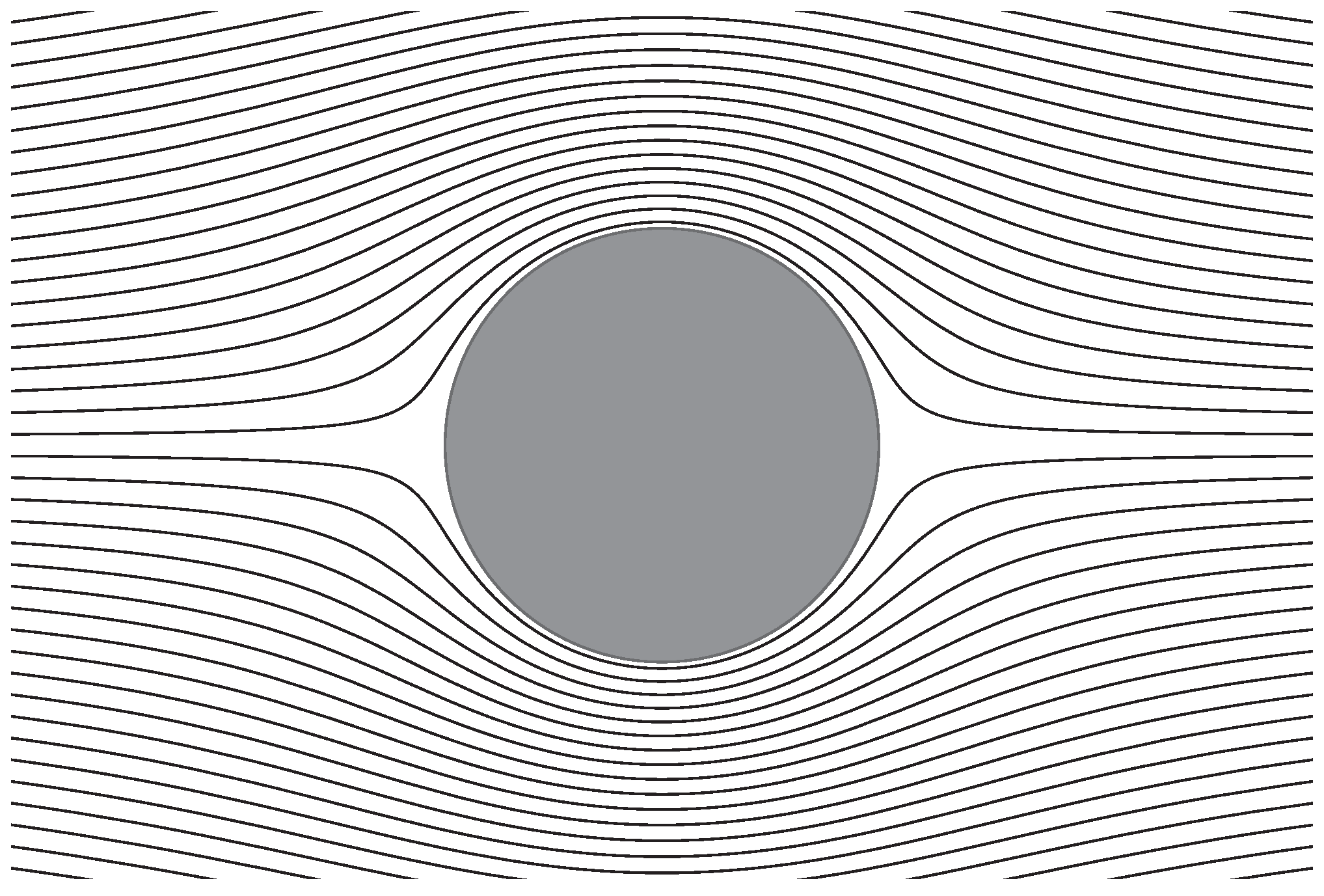
Figure 2 shows streamlines in the symmetry plane.
From this figure, it is obvious that there are two stagnation points on two sides of the sphere [14,15]. The flow is separated by the stagnation lines attached to the stagnation points on the sphere.
According to the stream functions and velocity fields, the Stokes force exerted on a rigid stationary spherical particle immersed in the uniform Stokes flow field is
By Newton’s law, when the sphere reaches its terminal velocity , the forces acting on the sphere are balanced. Thus, the magnitude of the terminal velocity U is
where g is the acceleration due to gravity and is the density of the sphere. Equation (7) is the Stokes law and can be further corrected by Faxén’s laws. Considering the Faxén correction, the drag on a stationary rigid sphere in the Stokes flow is
The second term comes from Faxén correction. However, if the sphere reaches its terminal velocity, , the terminal velocity is the same as (8).
3.2. Uniform Flow past a Fluid Drop
If the rigid sphere discussed above is replaced by a spherical fluid drop of radius d, i.e., the radius of the rigid kernel, a, is zero in Figure 1, this is the case for uniform flow past a fluid drop. The fluid of the drop is immiscible with the surrounding fluid and the interface is spherical. The fluid drop is moving at a constant speed through the surrounding fluid without changing its shape [37,38], or the flow is past a fixed, undeformed fluid drop. The most general expressions for the stream functions outside and inside the drop [36] are
and
respectively. Here, A, B, C, D, , , , are unknown constant coefficients. From the stream functions, the velocity fields and stress tensors can be deduced with specified boundary conditions.
In the region outside the drop, the fluid velocity is asymptotic to as .
On the drop boundary, the normal velocity is zero, , which implies
Inside the drop, the fluid velocity must remain finite as , i.e.,
and , which requires
Two additional constraints—continuity of tangential velocity and continuity of tangential stress—are required at the interface of the two fluids. These constraints set
and
After solving the above Equations (12)–(17), the coefficients in the stream functions are determined as
Thus, the stream functions outside and inside the drop are
and
respectively. This result is known as the Hadamard–Rybczyński equation [39]. Figure 3 shows streamlines in the symmetry plane for uniform flow past a fluid drop.
In the limit, , in which the drop is much more viscous than the surrounding fluid, Equation (4) is recovered from the stream functions (19) and (20).
The drag on the fluid drop is predicted as
If the drop is falling in fluid, it reaches the terminal velocity when the forces exerted on it are balanced. So, the magnitude of the terminal velocity is
where is the kinematic viscosity of the surrounding fluid.
3.3. Uniform Flow past a Rigid-Kernel Sphere with a Fluid Coating
For uniform flow past a rigid sphere with a fluid coating, we make similar assumptions for boundaries as in the above cases. First of all, the rigid spherical kernel with fluid coating remains spherical. Both fluids are Newtonian and mutually immiscible, and there is no interfacial mass transfer (the radial velocity is zero at the interface). Following (10) and (11), the general stream functions are proposed as
in which A, B, ⋯, are constant coefficients. Consequentially, for ,
For ,
To determine the unknown coefficients in Equations (23) and (24), we impose the boundary conditions. Boundary conditions are evaluated at the fluid-fluid interface , and the interface of the rigid spherical kernel and the fluid coating .
- The boundary condition at infinity implies
- The zero normal velocity at the interface of fluids sets
- With the continuity of tangential velocity at the interface of fluids, the following equation is satisfied
- The no-slip boundary condition at requires
- Continuity of tangential stress at the interface of the fluids implies
Finally, combining Equations (31)–(35), we solve for the constant coefficients. The constant coefficients are attained as
where
Thus, the stream functions for the flow outside the particle and the flow inside the coating, Equations (23) and (24), are determined:
Figure 4 shows the streamlines of the fluid field outside the object and inside the fluid coating. For this figure, the radius of the rigid kernel , the thickness of the fluid coating , and the viscosity ratio of two fluids is .
In the limit of high viscosity stratification , Equation (4) is recovered from the stream functions (37) and (38). Even if the viscosities of two fluids are the same, , the streamline pattern for this special case is still similar to the general situation shown in Figure 4. The stream functions are simplified as
The discontinuity in the radial stress across the fluid–fluid interface is related to the surface tension of the interface at
where α is the surface tension [36,39]. As long as the drop moves at the constant terminal velocity U, all constraints at the interface between the two fluids are completely satisfied. This fact validates the previous assumptions that the interface is spherical and the drop moves constantly through the surrounding fluid at a constant speed without changing its shape. This is different from the sphere coated with a thin film studied by Johnson [19]. For the thin film results, the surface tension force is larger than the viscous force, and “the mechanism driving the fluid circulation within the film is not too large.” The radial velocity in the thin film is assumed to be one order lower than the tangential velocity for the asymptotical analysis. Furthermore, global force equilibrium has also been proposed for the thin fluid film. The above assumptions are relaxed in our problem. The compound particle is held as spherical with enough surface tension. However, the surface tension in Equation (39) may be significant and is important for the stability of the problem. It would be important to further analyze the stability and the Magrangoni effect—which is totally neglected—in the future work.
3.4. Hydrodynamic Drag Force and Terminal Velocity
Hydrodynamic drag force is of fundamental interest for the flow being examined. The drag force is evaluated by integrating the surface stress vector over the body surface. For this axisymmetric problem, the integration can be carried out explicitly.
According to the results (37) and (38), the Stokes force exerted on a stationary spherical particle immersed in the uniform Stokes flow field U are
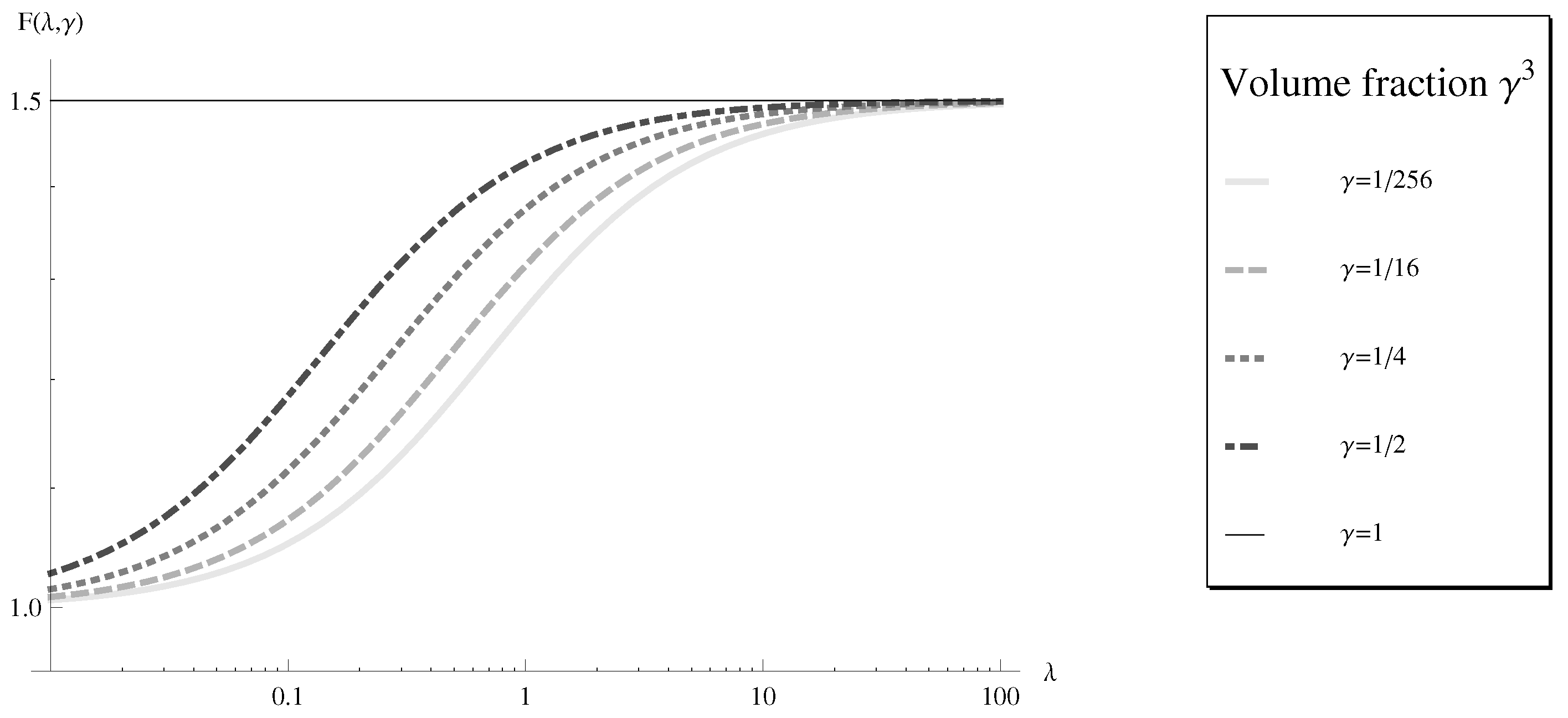
Note the viscosity ratio as and the volume fraction in terms of ratio . After nondimensionalizing the drag with a dimensional factor , the non-dimensional drag force is
Figure 5 and Figure 6 show the dimensionless drag with one variable fixed. Figure 5 demonstrates the dimensionless drag as a function of the viscosity ratio λ with the volume fraction fixed. With the fluid coating, the object experiences less drag on it. The outcome is consistent with other studies [19,26]. When the viscosity ratio approaches the limit , the object behaves likes a rigid sphere with radius R, which implies the volume framce case. The drag force satisfied the Stokes drag Equation (7) reviewed in Section 3.1.
The dependence of the dimensionless drag on the volume fraction is depicted in Figure 6. In the limiting case of , the result for the solid sphere is recovered. Given the viscosity ratio λ, the dimensionless drag force decreases if the volume of the fluid coating increases. When the viscosity ratio is small and the volume fraction goes to the limit , the result is asymptotic to the fluid drop result (21) in Section 3.2.
When the sphere reaches its terminal velocity U, the forces acting on the sphere are balanced, i.e.,
Here, ρ, and are density for the background flow, the fluid coating and the rigid kernel, respectively. Applying the results for hydrodynamic force in (40) to (42), we can calculate the terminal velocity of such a freely falling spherical object
To compare the terminal velocity of this compound particle with a rigid sphere or a fluid drop, the densities of the fluid in the coating and the rigid kernel are both set as the mean density . Therefore, their masses and volumes are the same. Then, from (43), the terminal velocity of the compound particle is
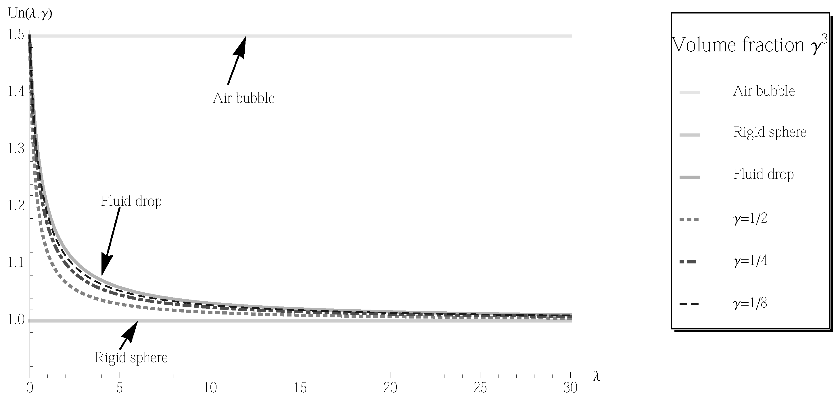
where . Nondimensionalize the terminal velocity,
in which is the terminal velocity of the corresponding rigid sphere from (8). Applying the same nondimensionalization, we know the terminal velocity of the rigid sphere and fluid drop are
Figure 7 shows the nondimensionless terminal velocities for those objects. With this figure, the transition and the asymptotic behavior to two limit cases, i.e., a rigid sphere and a fluid drop, are demonstrated well. It is interesting to see that by selecting the volume fraction and viscosity of fluids, the designed terminal can be targeted. This is an important feature for the drug delivery applications.
3.5. Multiple-Layer Fluid Coating
Under similar assumptions for the particle and the properties of fluids, we assume the rigid kernel is covered by two or three layers of fluid coating. Between adjacent layers, boundary conditions (32)–(35) hold with their corresponding fluid viscosities. The same type of stream function is proposed in each fluid coating layer. When a new layer is added, four more unknown coefficients are introduced in the stream function. These four coefficients are coupled with the coefficients in the stream function of the fluid coating layer(s) next to it. To solve this fluid problem, a linear system for the unknown coefficients is constructed. When the unknowns are arranged in a particular way, a block tridiagonal matrix arises. The reason to arrange the unknowns in a certain order is to achieve the resulting efficiencies. For example, solution algorithms are most efficient if these patterns are taken into account in the LU decomposition. Once we obtain the unique coefficients, the analytical formulae for the stream functions can be written out. Further analysis about the flow field is possible.
For a sphere with a rigid kernel and one layer of fluid coating discussed before (, see Figure 1), the linear system is the combination of Equations (31)–(35):
It is easy to see that we can eliminate the unknowns and , even for the other cases. However, they are saved to illustrate that the number of unknown coefficients grows arithmetically and four unknown coefficients are associated with each fluid layer, even the unbounded region outside the particle. As the determinant of the coefficient matrix is not equal to zero, the system is invertible. The coefficients are uniquely determined and the solution is non-trivial as documented in Equation (36).
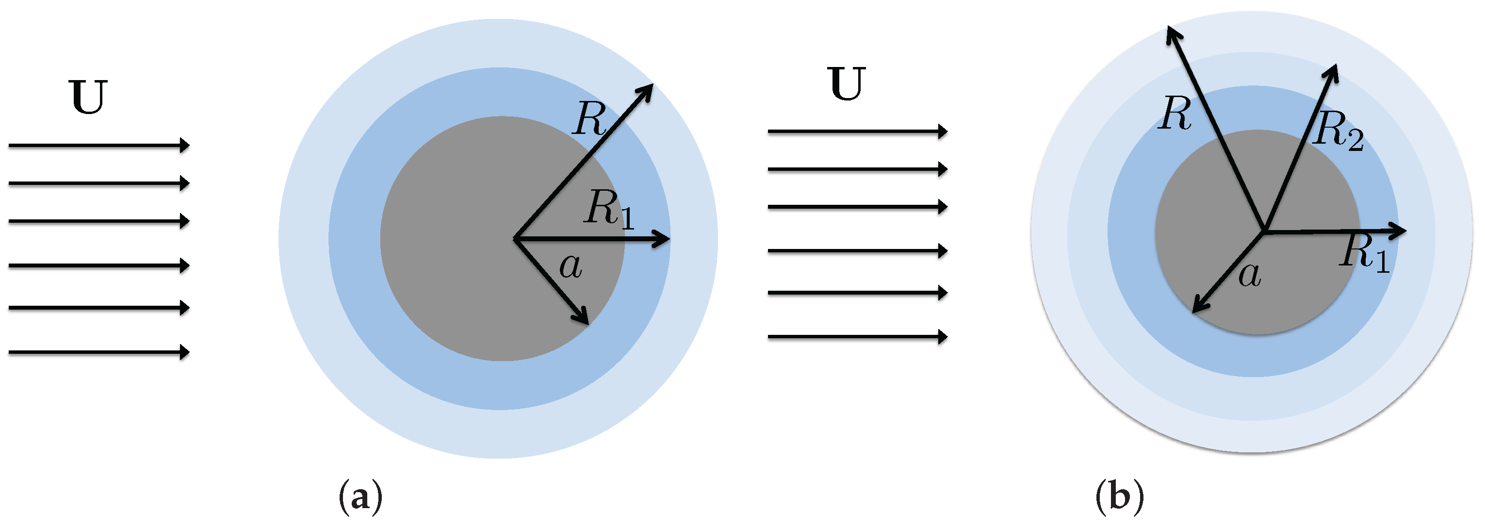
For a spherical particle with a rigid kernel and two-layer fluid coating, Figure 8a shows the diagram of the problem. Radii for the fluid coating satisfy . Keep for the stream function outside the particle and for the inner layer next to the rigid kernel, as the previous case. Note as the coefficients for the stream function of the outer layer (). The viscosity of fluid outside the particle is μ; is the viscosity of the fluid in the layer , and the new parameter is for the fluid in the layer . To attain the analytical solution, we collect the boundary conditions in terms of the unknowns. The linear system for the unknowns is
where the coefficient matrix is
![Fluids 01 00036 i001]() and
and

The entries in terms of the new layer radius are highlighted in the matrix, and the block matrices on the diagonal are marked out. The coefficient matrix can be viewed as a block tridiagonal matrix.
For a spherical rigid kernel covered with a three-layer fluid coating as shown in Figure 8b, radii of the fluid coating satisfy . Compared to the linear system (47), four more unknowns are introduced. The coefficient matrix for the corresponding linear system is
![Fluids 01 00036 i002]()

The entries in terms of the new layer radius are highlighted in the matrix. Since the determinant of this coefficient matrix is not equal to zero, the unknown coefficients in the stream functions can be uniquely determined.
The above results show the analytical solution, i.e., the stream function, is well defined when we propose the ideal conditions for the fluids and boundaries. In reality, these conditions may not be physical preferred. However, such solutions could be used as the fundamental solution to further explore the complicated situations. In general, we can keep adding more layers to the fluid coating. The solvability for a general N-layer fluid coating is an interesting linear algebra problem and will be reported in a future study.
4. Summary and Future Directions
In this paper, we have studied a uniform flow past a spherical compound object in the Stokes regime. The object consists of a rigid kernel with a fluid coating. Rigorous analytical solutions are presented for different cases. The explicit stream functions are derived for both the fluid flow outside the object and the fluid flow inside the coating layer. The resulting plots of the streamlines show the circulation inside the fluid coating. From the stream functions, we obtained the explicit drag force and discussed terminal velocity of the object.
The results show that, given a fixed size, the spherical object, with a rigid kernel and covered with a fluid coating, experiences less drag than a pure rigid object, if they have the same mass and same volume. This finding is valuable to biomedical applications, as drag is closely related to the energy required to keep the object in motion.
This study is fundamental. The analytical results provide the basis to investigate the stability of the problem. With the exact solutions, the study of flow patterns can be extended to the bifurcation of the flow field and the Marangoni effect can be further explored. Such analytical results will also be critical to a future study of more complicated systems. For example, results reported in this paper will provide the solution for fluid in which chemical reactions are coupled with hydrodynamics when oxygen is pumped in flow past an oocyte [32].
Conflicts of Interest
The author declares no conflict of interest.
References
- Marconi, U.M.B.; Puglisi, A.; Rondoni, L.; Vulpiani, A. Fluctuation-dissipation: Response theory in statistical physics. Phys. Rep. 2008, 461, 111–195. [Google Scholar] [CrossRef]
- Millikan, R.A. On the elementary electrical charge and the avogadro constant. Phys. Rev. 1913, 2, 109–143. [Google Scholar] [CrossRef]
- Schirber, M. Landmarks. Physics 2012, 5, 9. [Google Scholar] [CrossRef]
- Seinfeld, J.H.; Pandis, S.N. Atmospheric Chemistry and Physics; John Wiley & Sons, Inc.: Hoboken, NJ, USA, 2006. [Google Scholar]
- McBain, S.C.; Yiu, H.H.; Dobson, J. Magnetic nanoparticles for gene and drug delivery. Int. J. Nanomed. 2008, 3, 169–180. [Google Scholar]
- Stokes, G.G. On the effect of the internal friction of fluids on the motion of pendulums. Trans. Camb. Philos. Soc. 1851, 9, 8. [Google Scholar]
- Brenner, H. The Stokes resistance of an arbitrary particle-IV Arbitrary fields of flow. Chem. Eng. Sci. 1964, 19, 703–727. [Google Scholar] [CrossRef]
- Hetsroni, G.; Haber, S. The flow in and around a droplet or bubble submerged in an unbound arbitrary velocity field. Rheol. Acta 1970, 9, 488–496. [Google Scholar] [CrossRef]
- Proudman, I.; Pearson, J.R.A. Expansions at small Reynolds numbers for the flow past a sphere and a circular cylinder. J. Fluid Mech. 1957, 2, 237–262. [Google Scholar] [CrossRef]
- Jeffery, G.B. The motion of ellipsoidal particles immersed in a viscous fluid. Proc. R. Soc. Lond. A 1922, 102, 161–179. [Google Scholar] [CrossRef]
- Wang, K.C.; Zhou, H.C.; Hu, C.H.; Harrington, S. Three-dimensional separated flow structure over prolate spheroids. Proc. R. Soc. Lond. A 1990, 421, 73–91. [Google Scholar] [CrossRef]
- Chwang, A.T.; Wu, T.Y. Hydromechanics of low-Reynolds-number flow. Part 2. Singularity method for Stokes flows. J. Fluid Mech. 1975, 67, 787–815. [Google Scholar] [CrossRef]
- Chwang, A.T. Hydromechanics of low-Reynolds-number flow. Part 3. Motion of a spheroidal particle in quadratic flows. J. Fluid Mech. 1975, 72, 17–34. [Google Scholar] [CrossRef]
- Zhao, L. Fluid-structure interaction in viscous dominated flows. Ph.D. Thesis, University of North Carolina at Chapel Hill, Chapel Hill, NC, USA, 2011. [Google Scholar]
- Camassa, R.; McLaughlin, R.M.; Zhao, L. Lagrangian blocking in highly viscous shear flows past a sphere. J. Fluid Mech. 2011, 669, 120–166. [Google Scholar] [CrossRef]
- Leal, L.G. Laminar Flow and Convective Transport Processes; Butterworth-Heinemann: Oxford, UK, 1992. [Google Scholar]
- Pozrikidis, C. Introduction to Theoretical and Computational Fluid Dynamics; Oxford University Press: New York, NY, USA, 1997. [Google Scholar]
- Mori, Y.H. Configurations of gas-liquid two-phase bubbles in immiscible liquid media. Int. J. Multiph. Flow 1978, 4, 383–396. [Google Scholar] [CrossRef]
- Johnson, R.E. Stokes flow past a sphere coated with a thin fluid film. J. Fluid Mech. 1981, 110, 217–238. [Google Scholar] [CrossRef]
- Harper, J.F. Surface activity and bubble motion. Appl. Sci. Res. 1982, 38, 343–352. [Google Scholar] [CrossRef]
- Sadhal, S.; Ayyaswamy, P.; Chung, J. Compound drops and bubbles. In Transport Phenomena with Drops and Bubbles; Springer: New York, NY, USA, 1997; pp. 403–442. [Google Scholar]
- Kawano, S.; Hashimoto, H. A numerical study on motion of a sphere coated with a thin liquid film at intermediate reynolds numbers. J. Fluids Eng. 1997, 119, 397–403. [Google Scholar] [CrossRef]
- Sagis, L.M.C.; Öttinger, H.C. Dynamics of multiphase systems with complex microstructure. i. development of the governing equations through nonequilibrium thermodynamics. Phys. Rev. E 2013, 88. [Google Scholar] [CrossRef] [PubMed]
- Sadhal, S.S.; Johnson, R.E. Stokes flow past bubbles and drops partially coated with thin films. Part 1. stagnant cap of surfactant film- exact solution. J. Fluid Mech. 1983, 126, 237–250. [Google Scholar] [CrossRef]
- Johnson, R.E.; Sadhal, S.S. Stokes flow past bubbles and drops partially coated with thin films. Part 2. thin films with internal circulation-a perturbation solution. J. Fluid Mech. 1983, 132, 295–318. [Google Scholar] [CrossRef]
- Gupta, B.R.; Deo, S. Axisymmetric creeping flow of a micropolar fluid over a sphere coated with a thin fluid film. J. Appl. Fluid Mech. 2013, 6, 149–155. [Google Scholar]
- Rushton, E.; Davies, G.A. Settling of encapsulated droplets at low Reynolds numbers. Int. J. Multiph. Flow 1983, 9, 337–342. [Google Scholar] [CrossRef]
- Li, X.; Pozrikidis, C. The effect of surfactants on drop deformation and on the rheology of dilute emulsions in Stokes flow. J. Fluid Mech. 1997, 341, 165–194. [Google Scholar] [CrossRef]
- Blawzdziewics, J.; Wajnryb, E.; Loewenberg, M. Hydrodynamic interactions and collision efficiencies of spherical drops covered with an incompressible surfactant film. J. Fluid Mech. 1999, 395, 29–59. [Google Scholar] [CrossRef]
- Datta, S.; Raturi, S. Cell model for slow viscous flow past spherical particles with surfactant layer coating. J. Appl. Fluid Mech. 2014, 7, 263–273. [Google Scholar]
- Fung, Y.-C. Biomechanics: Circulation; Springer Science & Business Media: New York, NY, USA, 1997. [Google Scholar]
- Somersalo, E.; Occhipinti, R.; Boron, W.F.; Calvetti, D. A reaction-diffusion model of co2 influx into an oocyte. J. Theor. Biol. 2012, 309, 185–203. [Google Scholar] [CrossRef] [PubMed]
- Klein, C.A. Cancer. The metastasis cascade. Science 2008, 321, 1785–1787. [Google Scholar] [CrossRef] [PubMed]
- Gusenbauer, M.; Kovacs, A.; Reichel, F.; Exl, L.; Bance, S.; Özelt, H.; Schrefl, T. Self-organizing magnetic beads for biomedical applications. J. Magn. Magn. Mater. 2012, 324, 977–982. [Google Scholar] [CrossRef]
- Nakhoul, N.L.; Davis, B.A.; Romero, M.F.; Boron, W.F. Effect of expressing the water channel aquaporin-1 on the co2 permeability of xenopus oocytes. Am. J. Physiol. Cell Physiol. 1998, 274, C543–C548. [Google Scholar]
- Batchelor, G.K. Slender-body theory for particles of arbitrary cross-section in stokes flow. J. Fluid Mech. 1970, 44, 419–440. [Google Scholar] [CrossRef]
- Rivkind, V.Y.; Ryskin, G.M. Flow structure in motion of a spherical drop in a fluid medium at intermediate reynolds numbers. Fluid Dyn. 1976, 11, 5–12. [Google Scholar] [CrossRef]
- Oliver, D.L.R.; Chung, J.N. Steady flows inside and around a fluid sphere at low Reynolds numbers. J. Fluid Mech. 1985, 154, 215–230. [Google Scholar] [CrossRef]
- Pozrikidis, C. Introduction to Theoretical and Computational Fluid Dynamics; Oxford University Press: New York, NY, USA, 2011. [Google Scholar]
Figure 1.
Uniform flow past a rigid sphere with a fluid coating. The background uniform flow is . The dark colored region indicates the rigid spherical kernel with radius a. The light colored region shows the fluid coating with thickness d. In total, the radius of the obstacle is .
Figure 1.
Uniform flow past a rigid sphere with a fluid coating. The background uniform flow is . The dark colored region indicates the rigid spherical kernel with radius a. The light colored region shows the fluid coating with thickness d. In total, the radius of the obstacle is .
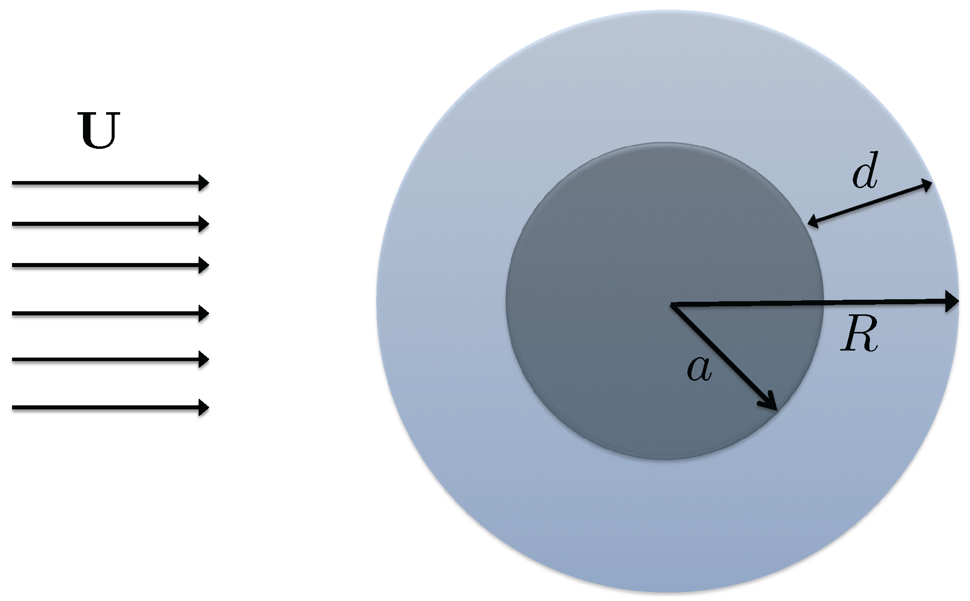
Figure 2.
Streamlines in the symmetry plane for a uniform flow past a rigid sphere. The radius of the rigid sphere is .
Figure 2.
Streamlines in the symmetry plane for a uniform flow past a rigid sphere. The radius of the rigid sphere is .

Figure 3.
Streamlines in the symmetry plane for uniform flow past a fluid drop. The radius of the fluid drop is and the viscosity ratio .
Figure 3.
Streamlines in the symmetry plane for uniform flow past a fluid drop. The radius of the fluid drop is and the viscosity ratio .
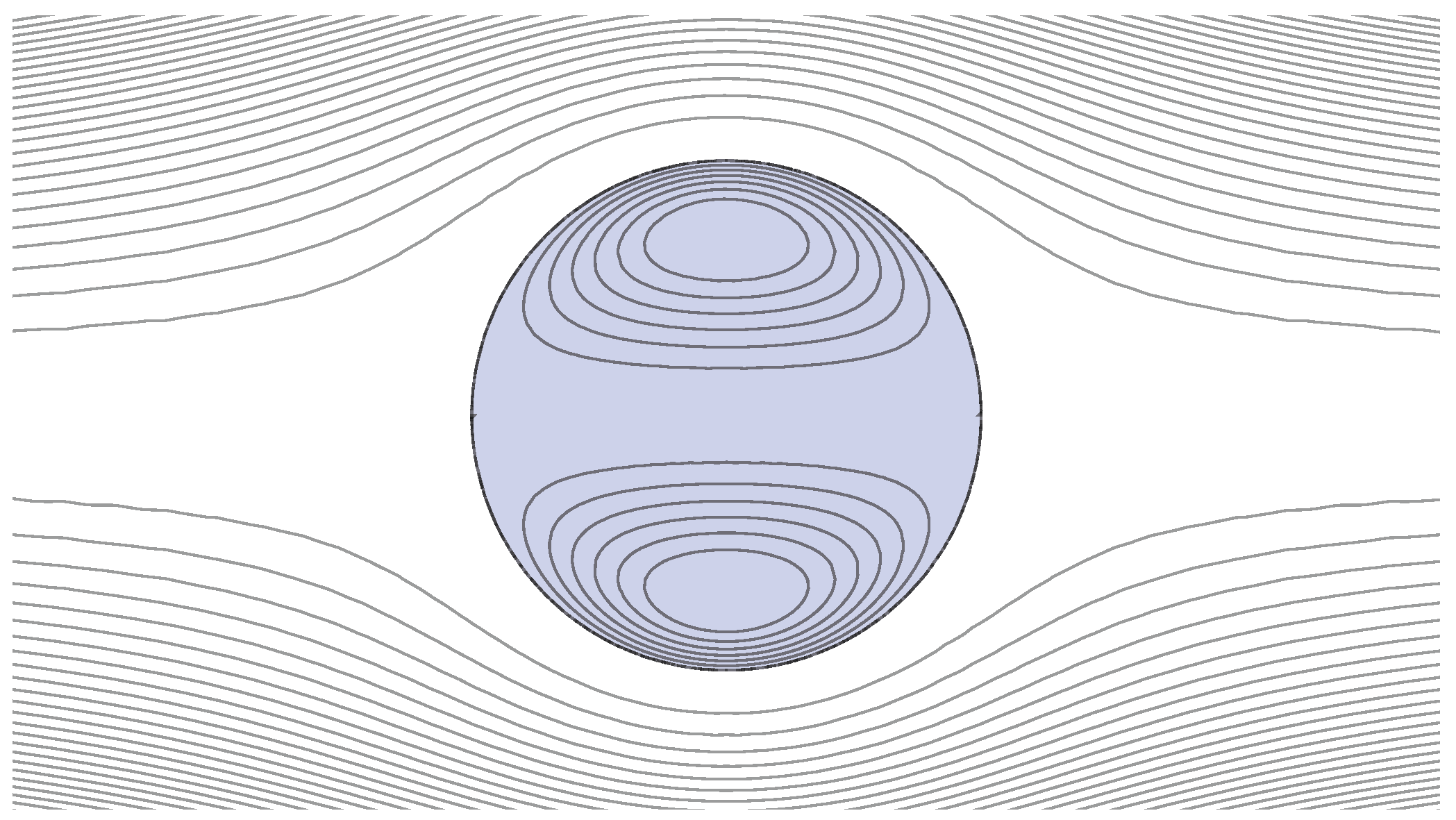
Figure 4.
Streamlines in the symmetry plane for the flow field of a uniform flow past a fluid-coated rigid-kernel sphere. The black region is the rigid kernel and the gray region with circulation is the fluid coating. The viscosity ratio is . The radius of the rigid kernel and the thickness of the fluid coating are set as .
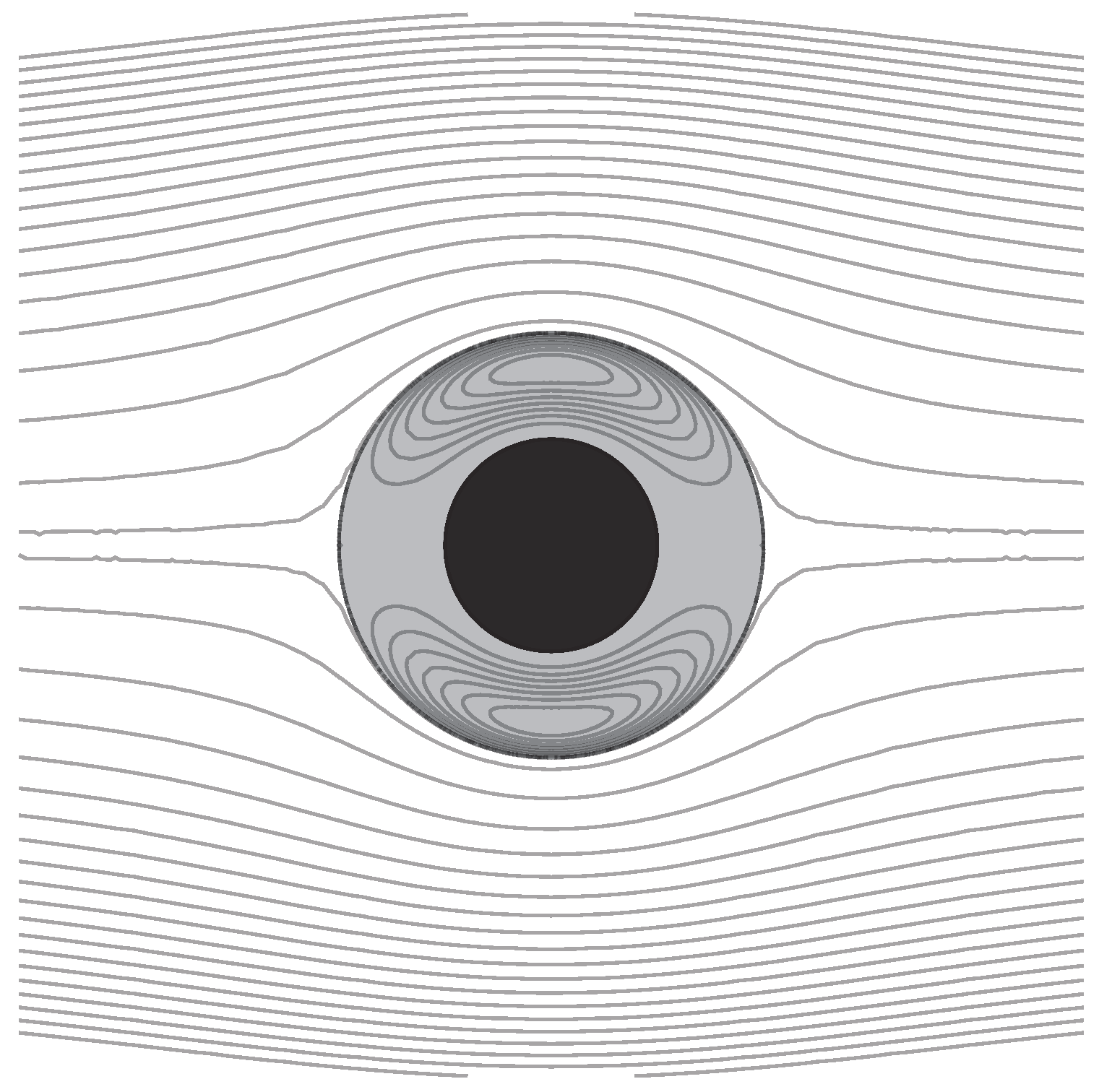
Figure 5.
Loglog plot of the dimensionless drag force as a function of the viscosity ratio λ with fixed values of the volume fraction, .
Figure 5.
Loglog plot of the dimensionless drag force as a function of the viscosity ratio λ with fixed values of the volume fraction, .

Figure 6.
The dimensionless drag force as a function of γ with fixed values of the viscosity ratio λ. is the volume fraction of the object.
Figure 6.
The dimensionless drag force as a function of γ with fixed values of the viscosity ratio λ. is the volume fraction of the object.
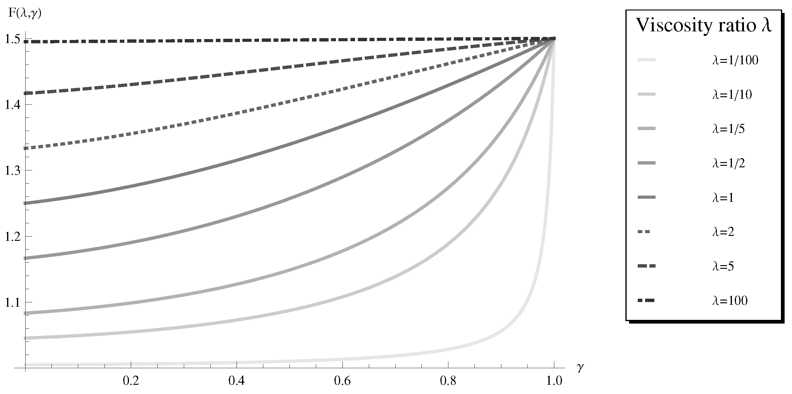
Figure 7.
The dimensionless terminal velocity as a function of the viscosity ratio λ with fixed volume fraction . The densities of the fluid in the coating and the rigid kernel are set be the same as the mean density . The radii of the two-layer object, the rigid sphere, the fluid drop, and the air bubble are the same. The air bubble result is obtained by taking the viscosity ratio for the fluid drop.

Figure 8.
The uniform background flow past a rigid sphere with a multiple-layer fluid coating. The gray region with radius a indicates the rigid kernel. The light colored regions show the fluid coating with radii , , and R for the three-layer case. (a) The rigid kernel covered with a two-layer fluid coating. ; (b) The rigid kernel covered with a three-layer fluid coating. .
© 2016 by the authors; licensee MDPI, Basel, Switzerland. This article is an open access article distributed under the terms and conditions of the Creative Commons Attribution license ( http://creativecommons.org/licenses/by/4.0/).
Share and Cite
MDPI and ACS Style
Zhao, L. Hydrodynamics of Highly Viscous Flow past a Compound Particle: Analytical Solution. Fluids 2016, 1, 36. https://doi.org/10.3390/fluids1040036
AMA Style
Zhao L. Hydrodynamics of Highly Viscous Flow past a Compound Particle: Analytical Solution. Fluids. 2016; 1(4):36. https://doi.org/10.3390/fluids1040036
Chicago/Turabian StyleZhao, Longhua. 2016. "Hydrodynamics of Highly Viscous Flow past a Compound Particle: Analytical Solution" Fluids 1, no. 4: 36. https://doi.org/10.3390/fluids1040036