
Meridional and Zonal Wavenumber Dependence in Tracer Flux in Rossby Waves

School of Mathematical Sciences, University of Adelaide, Adelaide, SA 5005, Australia
Fluids 2016, 1(3), 30; https://doi.org/10.3390/fluids1030030
Submission received: 22 July 2016
/
Revised: 26 August 2016
/
Accepted: 29 August 2016
/
Published: 6 September 2016
(This article belongs to the Collection Geophysical Fluid Dynamics)
Abstract
:Eddy-driven jets are of importance in the ocean and atmosphere, and to a first approximation are governed by Rossby wave dynamics. This study addresses the time-dependent flux of fluid and a passive tracer between such a jet and an adjacent eddy, with specific regard to determining zonal and meridional wavenumber dependence. The flux amplitude in wavenumber space is obtained, which is easily computable for a given jet geometry, speed and latitude, and which provides instant information on the wavenumbers of the Rossby waves which maximize the flux. This new tool enables the quick determination of which modes are most influential in imparting fluid exchange, which in the long term will homogenize the tracer concentration between the eddy and the jet. The results are validated by computing backward- and forward-time finite-time Lyapunov exponent fields, and also stable and unstable manifolds; the intermingling of these entities defines the region of chaotic transport between the eddy and the jet. The relationship of all of these to the time-varying transport flux between the eddy and the jet is carefully elucidated. The flux quantification presented here works for general time-dependence, whether or not lobes (intersection regions between stable and unstable manifolds) are present in the mixing region, and is therefore also easily computable for wave packets consisting of infinitely many wavenumbers.
1. Introduction
Rossby waves are ubiquitous in the atmosphere and ocean, and arise from the Earth’s rotation and curvature [1,2]. Their structure is often associated with meandering jets of a large horizontal extent, with mesoscale eddies within the meanders [3,4,5,6,7]. The term “eddy” shall be used throughout this paper for these rotating structures as a generic identifier; in context, this could represent a “vortex”, “ring”, “hurricane” or “cyclone”. Classically, Rossby waves are obtained from the conservation of potential vorticity (PV), and a one-mode Rossby wave provides an excellent first-order approximation to meandering (eddy-driven) jets, which have a dominant zonal and meridional spatial scale [1,2,3,8,9,10].
Crucial to the understanding of transport in the atmosphere and oceans is the presence of nominal transport barriers between coherent structures. These can be, for example, an oceanic front, the “edge” of the Antarctic circumpolar vortex, the boundary between an eddy and an adjacent jet in the ocean, the boundary between a cyclone and a mid-latitude jet, etc. One can think of these as barriers between mesoscale “Lagrangian coherent structures” (LCSs), although there is confusion in this nomenclature since these barriers themselves are sometimes called LCSs [11]. These are only “nominal” barriers in the sense that transport does occur across these, which makes it difficult to define exactly what the “barrier” is (this paper will offer some resolution to this issue under certain circumstances). Nevertheless, understanding the interchange of fluid, PV, heat, salinity, nutrients, pollutants, energy, phytoplankton, etc., across these barriers is vital in evaluating the role of LCSs in the transport of these scalar quantities. The fact that the LCSs, and their boundaries, are themselves moving with time in arbitrary ways makes this proposition quite difficult. One diagnostic often used in oceanography and the atmospheric sciences to attempt to determine these barriers is seeking strong ridges of finite-time Lyapunov exponent (FTLE) fields or the closely related finite-size Lyapunov exponent fields [12,13,14,15,16,17,18,19,20,21,22,23,24]. These barriers are also sought via many other methods, of which a non-exhaustive list is the hyperbolic LCS method of Haller [11], averaging applied to parcel trajectories [25,26,27,28], topological entropy of braids from intermingling Lagrangian trajectories [29,30], curves of least curvature deformation [31], exit/residence time fields [22,32], transport characterization using Perron-Frobenius operators [33,34,35,36], and a direct identification as stable/unstable manifolds [37,38,39,40,41]. A note of caution: Eulerian fields (e.g., instantaneous PV contours, Okubo-Weiss criterion, etc.) are well-known to give an incorrect understanding of Lagrangian transport in genuinely unsteady flows [11], and thus shall be avoided here.
The exact conservation of PV imposes topological constraints which inhibit mixing between the jet and adjacent eddies [42,43]. In other words, the flow barrier between the coherent entities (the jet, and an adjacent eddy) remains impervious. Mixing is therefore associated with dynamically-relevant disturbances which break the conservation of PV. An early study by Pierrehumbert [3], in which a weakly PV-conserving disturbance was added, demonstrated that chaotic mixing would result (while the PV was conserved for both the dominant and the weak modes individually, it is only weakly conserved for their sum since the PV conservation equation is nonlinear). Many similar early studies, but with differing dynamical considerations [44,45,46,47,48,49], reached comparable conclusions. In all these cases, the disturbance was time-periodic, and it is now well-established that in such instances, chaotic mixing is the generic expectation [12,41,50,51,52]. This line of study continues to be popular [20,53,54,55]. Time-aperiodicity is a different proposition, since it disallows the principal dynamical-systems tools for analysing chaotic mixing used in the above mentioned studies: Poincaré maps which sample the flow at the period of the disturbance [46,47,49,51,54,55]. Nevertheless, there have been attempts to adapt the classical methodology for assessing transport in these situations [56,57,58,59]. These usually rely on quasi-periodicity and/or the possibility of identifying lobes of fluid in the chaotic region, whose areas are linked to transport. In realistic flows, however, very general time-variation is present, e.g., [60], for which a consistent theory would be valuable.
The intersections between dynamical-systems entities called stable and unstable manifolds are now well-known to be an instigator of mixing between coherent regions in fluid flows [12,41,46,61,62]. These can indeed be construed as the time-dependent “barriers” discussed previously [39]. A recent restatement of their role in transport is that these are crucial flow separators in forward and backward time respectively [32]. Complicated intersections between stable and unstable manifolds at a particular instance in time identify regions in which large chaotic mixing is happening [49,51], but it must be borne in mind that in a genuinely unsteady flow, these entities are moving around with time. The regions bounded by intersections are called “lobes” and are the basis of the classical lobe dynamics approaches to quantifying transport in fluids [49,51]. However, lobes need not exist in general time-aperiodic situations because it is possible for stable and unstable manifolds to not intersect; this is indeed generic when introducing dissipation into a geophysical flow [37,38,41]. Even if they do exist in a general time-varying flow, it is difficult to rationalize exactly how they transfer fluid between, say, an eddy and the jet, and when the transfer happens.
Most transport studies that work with the Lagrangian trajectories focus on fluid flux. However, understanding scalar fluxes of many other quantities—such as heat, pollutant, energy, plankton, nutrients and potential vorticity [23,56,63,64,65,66,67]—is often of interest. One contribution of the present article is to provide a method for quantifying both the fluid and tracer flux between an eddy and the jet as a time-varying entity, without having the need to identify lobes, or even for lobes to exist. This enables the determination of fluid/tracer flux for disturbances that are not time-periodic, for example consisting of wave packets with zonal and meridional wavenumbers distributed either discretely or continuously [68]. The computability of the flux in such situations is presented in Section 3.3. This new tool is anticipated to have applicability in other situations, for example in determining the future depletion of an eddy subject to wave packets with wavenumbers normally distributed around known stable values.
The second goal of this article is to specifically determine wavenumbers that provide extremal (maximal or minimal) chaotic mixing between a jet and an eddy, while being subject to Rossby wave dynamics. This is in the spirit of Farrell [69], who investigated wavenumbers that resulted in the most growth, and Barnes and Hartmann [7], who addressed the vorticity stirring power as a function of meridional wavenumber for the mid-latitude eddy-driven jet; here the focus is on the most eddy-jet transport. These disturbances can arise from dynamical or physical considerations (e.g., the most stable modes [70]), wind-forcing on the ocean surface [60], or eddy diffusivity [63]). For a specific choice of wavenumbers, it is possible to view the resulting mixing [3,45], or to obtain measures of mixing [3], by numerically advecting many particles using either direct advection of parcel trajectories, or advection-diffusion of a tracer field. Having performed such a computation (for which a time-interval would need to be specified), tools such as the finite-time Lyapunov exponent (FTLE) [9,12,32,54,71], mix-norm [72], effective diffusivity [73,74,75], network complexity [36] or topological entropy [29,30]—to name a few—can then be used to quantify mixing. Each such computation—for a specific chosen zonal and meridional wavenumber, and a chosen time-interval—would be tractable but relatively expensive. Using a method like this to search the parameter space for wavenumbers that maximize eddy-jet transport is therefore prohibitive. A tool that can quickly identify the most and least influential wavenumbers for mixing would be highly useful. This study provides exactly that, and is able to tune it based on the geometry of the dominant meandering jet and the local planetary parameter. The optimally-mixing zonal and meridional wavenumbers turn out to be distributed in a non-uniform and non-obvious manner, illustrating that this tool is indeed valuable.
The methods developed in this paper may allow for the investigation of many interesting issues. Could low energy excitations at optimally-mixing wavenumbers be used to maximize transport between an eddy and a jet? Alternatively, which geometry of meandering jet, and occurring at what latitudes, would be most effective at causing eddy-jet mixing due to the presence of white noise perturbations? Is it possible to determine wave packet disturbances that can cause an eddy to deplete very rapidly? If wavenumbers are gathered from an atmospheric or oceanic situation (by applying spatial Fourier transforms to observational data, say) at some instance in time, can this be used to predict eddy-jet transport into the future? Can the flux into/out of a mid-latitude cyclone be determined from observed poleward momentum surges [8,76]?
This paper is organized as follows. Section 2.1 sets the stage by introducing the dominant Rossby wave which is associated with a meandering jet with flanking eddies. This is an exact solution to PV conservation dynamics, and reflects a situation in which there is no flux between the jet and an adjacent eddy. Section 2.2 explains how fluid and tracer fluxes can be defined as time-varying quantities. These definitions do not require the velocity field to be perturbative, that is, that it be represented by a dominant stream function to which is added a disturbance. Neither do the definitions necessitate any particular specification on the dynamics of how the tracer field evolves. Thirdly, the time-dependence can be very general (e.g., Rossby wave packets). This process in fact enables a definition of what the “barrier” is in this situation in which there is actually non-zero transport across the so-called barrier. Appendix A provides a detailed discussion on the relationships between the flux as defined here, and classical transport quantifiers (lobe dynamics, width of chaotic layer, etc.), which are applicable in less general situations. Section 3.1 specializes the flux formula for the case where a dominant Rossby wave is disturbed by a linearized Rossby mode. This permits the development in Section 3.2 of a methodology for determining the zonal and meridional wavenumbers that maximize transport between the chosen eddy and the jet. The predictions obtained from this are validated by using both FTLEs and numerical computations of stable and unstable manifolds. Section 3.3 provides flux calculations for several wave packet situations, and Section 4 discusses avenues for future continuation of this work.
2. Materials and Methods
2.1. Rossby Waves
A flow dominated by one Rossby wave can be represented by the stream function [3,6,10,12,54,57,69,77]
in which are the local eastward and northward coordinates, and are the wavenumbers in these directions, and . This stream function is associated with a Rossby wave with wavelength propagation only in the eastward direction, with its northern meanders being delimited by the value of . This is dynamically consistent in that (1) is an exact solution to the barotropic potential vorticity conservation equation [3], that is, the equation
where the barotropic potential vorticity (PV) is defined by
The quantity is the linearized effect of its change when moving to nearby latitudes. All variables with primes are dimensional, in contrast to nondimensional variables which shall be unprimed. Fluid parcel trajectories associated with this satisfy
Thus, (2) is an explicit statement that the PV is conserved following parcel trajectories of (4). Variables shall be changed to nondimensional ones which are stationary in the frame of reference of this wave. To this end, define nondimensional (unprimed) variables by
(It proves convenient to use the wave speed c as the nondimensional parameter, noting that it encodes information about .) In these new variables, the parcel trajectories obey
where the nondimensional stream function
incorporates both a scaling with respect to and a translation to the x frame of reference, and is now independent of time. For (i.e., for the dimensional planetary parameter satisfying ), the streamlines associated with (6) display a meandering jet with eddies on the side as shown in Figure 1. The jet travels eastward in this frame of reference, with the eddies rotating clockwise. If , the picture is similar in spirit, but with all directions of flow reversed. If , there are no eddies (the meandering jet extends meridionally). The case is a degenerate transition; the eddies present for shrink and disappear when exceeds 1. The jet disappears at ; there are then square cells of alternating vorticity (the Taylor-Green flow [52]).
Here, the generic situation of when is the focus; Figure 1 has been produced with (associated with realistic parameters for a typical atmospheric mid-latitude cyclone as reported by Oruba et al. [9], to be discussed in detail later). The dimensional wavenumbers are associated with the zonal and meridional reciprocal length scales of the eddy. In this case, the darker curves demarcate the boundaries between the jet and the eddies, across which there is no transport. This sort of qualitative behavior is common in many other dynamically-inspired or kinematic studies [44,45,46,47,55,78].
The goal is to capture the flux between the eddy in the southwest corner of Figure 1 and the main jet as a function of time, resulting from the presence of a dynamically relevant disturbance in the stream function. In other words, this is the flux across the heavy magenta curve in Figure 1, denoted Γ. This curve is the stable manifold of the saddle fixed point at the southeastern corner of the eddy. This is defined by the set of fluid parcels which in forward time approach . It turns out that this occurs exponentially slowly, since the velocity is zero at the saddle point. However, Γ is also the unstable manifold of the saddle fixed point at the southwestern corner of the eddy. That is, parcels on Γ approach as . Since Γ comprises a curve in which a stable manifold coincides with an unstable manifold, it is a heteroclinic manifold [51,79]. In this case, it is identifiable also as part of the level set . In this steady situation, being on either side of Γ unequivocally determines whether a fluid parcel is within the eddy or the jet.
The full (dimensional) flow will therefore consist of the dominant Rossby mode, plus a disturbation, i.e., fluid parcels will obey
with stream function
In contrast to in which the time-dependence disappears when converted according to (5), will in general have arbitrary time-dependence. In general, one can think of the dimensional stream function consisting of a wave packet comprised with a finite or infinite number of Rossby waves. If limiting attention to countable waves, it would have the form
in which the wave speed of each mode obeys
for dynamical consistency. The coefficients are assumed small in comparison to in thinking of this as a disturbance on the dominant wave whose transport characteristics are shown in Figure 1. The sum in (10) may be over a finite number of wavenumbers , or an infinite number, and the “smallness” of the coefficients can be set with the requirement
More general wave packets in which the wavenumbers vary continuously are also allowable. That is,
where the wave speeds satisfy (11) (the wavenumber is disallowed, since there is no well-defined wave speed in (11) for this specific wavenumber), and with requirements on the coefficient functions to ensure that the improper integral (12) converges. Moreover, (12) must be a perturbation on the dominant stream function . These requirements can be combined by insisting on
There may be restrictions on the wavenumbers in the perturbing stream function (10) or (12) depending on the problem at hand. In an “open ocean/atmosphere” model there may be no restrictions. If the eastward spatial periodicity is to be preserved (for comparison with a numerical solution of the PV Equation (2) generated using periodic boundary conditions, say), then should be restricted to integer multiples of . As another example, in a channel-flow model with vertical boundaries and , and all possible s would be restricted to taking values that are integer multiples of . In this article, a particular restriction shall not be imposed; the methodology presented for finding flux and flux-optimizing wavenumbers can easily be restricted to any such case if needed. In either of the forms (10) or (12), the -dependence will not in general be periodic or quasi-periodic. Moreover, the possibility of dealing with wave packets such as these is a first step to determining the flux occurring due to stochastic perturbations, for example by choosing the εs from an appropriate random distribution.
Next, the same nondimensional transformation of coordinates, as given by (5) needs to be applied to the disturbance stream function. This will result in fluid parcel trajectories being described by
with nondimensional stream function
It is worth reiterating that the nondimensional disturbance stream function obtained from (10) or (12) will have arbitrary t-dependence. Now, the quantification of the tracer/flux flux occurring across Γ in Figure 1 is a non-trivial exercise given that the barrier breaks up into two different entities: a stable manifold and an unstable manifold, which do not coincide in general. They may intersect at infinitely many times, finitely many times, or even not at all. Moreover, these structures will be moving with time. The “flow barrier” therefore consists of a region in which these stable and unstable manifolds intermingle. It is indeed not an impermeable flow barrier (unlike in Figure 1), but a “barrier-region” across which transport does occur between the jet and the eddy. Defining what transport means in this context requires usage of recently developed dynamical systems methods, as are outlined in Section 2.2.
2.2. Fluid and Tracer Flux
In unsteady flow situations, the unambiguous flux barrier Γ in Figure 1 breaks apart, into a separate stable and an unstable manifold. These need not coincide, and typically will exhibit complicated intersections when viewed at any time. The fact that the stable and unstable manifolds are themselves moving with time makes the identification of a “flux” doubly difficult. This section will outline an emerging viewpoint on characterizing the flux which:
- allows for the disturbance to have any time-variation;
- explicitly quantifies the flux as a function of time;
- does not care whether manifolds intersect zero times, a finite number of times, or an infinite number of times;
- captures both simple and complicated (chaotic) forms of transport; and
- works for compressible two-dimensional flows (geophysical fluid might need to satisfy volume preservation, and so when observing behavior on two-dimensional sheets (e.g., isopycnals), area-preservation need not be satisfied since the isopycnals can compress towards one another).
While this section provides an intuitive description of the flux-quantification approach, more theoretical details and connections to other methods are discussed in Appendix A.
Consider first fluid flux. Under the influence of the unsteady disturbance, the unstable manifold emanating from in Figure 1 persists, but now as the time-varying unstable manifold of a specialized trajectory which moves around while continuing to lie on near to . This trajectory shall be referred to as an anchoring trajectory since the manifold is anchored to this (see Appendix A for a more rigorous understanding as to what this trajectory is). A picture of this, at a time t, could possibly be like Figure 2, where the unstable manifold is shown in red. Similarly, perturbs to an anchoring trajectory whose stable manifold is shown in green. The trouble is that the previously coincident stable and unstable manifolds have now split up into two different entities. How can the a boundary between the eddy and the jet be thought of now? How can a transport between them be quantified?
One “obvious” approach might be to think of using an Eulerian definition of flux across Γ. Such an Eulerian flux associated with (13) at any instance in time t is easily represented by
where is a unit normal vector to Γ at each location. This is not a good measure because of a variety of reasons. It is well-known that examining Eulerian characteristics failsl in general to give proper Lagrangian information. This can be illustrated via several simple thought experiments. If the disturbance stream function retains the fact that the stable and unstable manifold coincide, then the definition should ensure that there is zero flux. However, if these coincide but at a slightly different location to that of Γ, (15) will give nonzero values. As another simple example, if the perturbed stable and unstable manifolds are both south of Γ in Figure 1, then (15) will be computing a flux from within the jet to within the jet, which is not what is of interest. Hence, a genuinely Lagrangian approach is necessary.
A simple-minded Lagrangian approach might be to compute the flux across a material curve, that is, a chain of particles, positioned for example on Γ, and then materially advected by the flow (13). The flux across this materially advected curve is always zero, since no fluid can cross the material curve. Thus, a “pure Lagrangian” approach cannot capture flux between the eddy and the jet. A method that is able to capture the antecedents of fluid parcels (whether within or outside the eddy), and also the transfer across the “barrier” which separates the eddy and the jet in the full flow (13), needs to be used.
Before introducing the more general method, a popular and attractive method that works for time-periodic situations (and with certain other restrictions) shall be briefly described. This is the lobe-dynamics approach to characterize chaotic mixing [49,51,80]. If the flow is time-periodic with period T, one can sample the locations of fluid parcels at times 0, T, , , etc. This can be thought of as strobing the flow, and the transition map between adjacent strobe times (say, from time 0 to T) is defined to be a Poincaré map [79], which shall be called P. Thus, P takes fluid parcels from Time 0 to time T, and since the flow is periodic with period T, indeed P would have the same action if considering times from, say, to . Now, if were zero, would be a fixed point of P. Moreover, points on Γ in Figure 1 will approach under repeated iterations of P. These points will be “jumping along’ Γ because P is a strobing of a continuous-time flow, but will in the asymptotic limit approach . Thus, Γ is ’s stable manifold with respect to the Poincaré map P. Similarly, Γ is ’s unstable manifold with respect to P. Now, if the disturbance stream function is small and time-periodic, it can be shown that the point , which would be immovable under P in the absence of a disturbance stream function, persists as a nearby fixed point of P when is small, and continues to have connected to it an unstable manifold [79]. Similarly, there will exist a fixed point of P to which is connected a stable manifold. The crucial issue now, however, is that this stable manifold need not coincide with the unstable manifold of . Generically, they will intersect non-tangentially at some point (imagine simply perturbing the two curves that were originally coincident; under almost any perturbation, one would expect an intersection). Call this point , which lies on both ’s unstable, and ’s stable, manifolds. Thus, , for any , must also lie on both the manifolds. Ergo, one intersection point implies infinitely many. Moreover, these points must satisfy the fact that and as , by virtue of being on the respective manifolds. This behavior is illustrated in Figure 2a.
Consider a lobe L as indicated in Figure 2a, which is defined by being a region of fluid bounded between intersecting stable and unstable manifolds. It is therefore subtended by two intersection points. After a time T, the fluid in this lobe must travel to another lobe , since its bounding curves must continue to be on the respective manifolds. Because of the fact that as , there is an accumulation of intersection points as one approaches . Thus, the intersection points which subtend the lobes get closer and closer, as the lobe approaches . To obey incompressibility, the lobe compensates by elongating in the complementary direction, as indicated in Figure 2a. Manifolds cannot self-intersect [79], and thus this elongated lobe for large n must stretch by a very large amount, which means it must then get pulled towards and consequently folded back up along the red unstable manifold. The next iterate, must be sandwiched between and the unstable manifold connecting to (not pictured here; this would be approximately along the y-axis, as seen in Figure 1), and so on. This results in an incredibly complicated stretching and folding of fluid parcels, which then re-enter the region near L to undergo the same process again. The inexorable “stretching” and “folding” process is one way to describe the process of chaotic mixing.
Given the complexity of motion, quantifying chaotic mixing is difficult. Rom-Kedar and collaborators [49,51] came up with the nice idea of lobe dynamics which applies in the scenario pictured in Figure 2a. There is no actual separator between the eddy and the jet in this instance; it has been split into two intermingling curves. Thus, they identify a nominal separator by considering the unstable manifold emanating from up to a point , connected to the stable manifold emanating from also connected to the same point . If one considers what crosses this pseudoseparatrix [49,51] after one iteration of P, it is seen that only the two lobes between and do so. (For example, P applied to takes it to L, which is on the same side of the pseudoseparatrix.) Thus, the area of a lobe can be used to quantify transport [49,51]. However, this area crosses under one iteration of P, i.e., during a time T, and thus a “better’ way of quantifying a chaotic flux might be to be this area divided by T [50]. Using these ideas relies on several other assumptions: there must be an intersection between the stable and unstable manifolds, all lobes must have equal areas to avoid having to decide which lobe to use, the fluid must be incompressible to ensure that has the same fluid area as L, the flow must be time-periodic to enable the definition of P, and moreover it must be time-periodic in a specific way to ensure that the picture of Figure 2a results (see Balasuriya [52] for time-periodic examples in which the lobe structure is irregular between and , unlike in Figure 2).
A method of quantifying transport where none of these assumptions are needed would be advantageous. This is by thinking of the stable and unstable manifold splitting not in terms of strobing the flow, but as a time-continuous variation [39,41,81]. A typical picture at an instance in time t is shown in Figure 2b. Here, is a specialized entity (which moves with time but remains close to ) to which is attached an unstable manifold. Similarly, there is a stable manifold attached to the entity , which is close to . Since all these entities move with time, Figure 2b shows only one instance in time. Consider the two fluid parcels labelled and . As time flows forwards, they will approach the (time-varying) because they are strongly impacted by the adjacent stable manifold. However, they cannot cross this (time-varying) stable manifold, which is a material curve. Thus, and will eventually arrive near to at some time , and then will get pulled by ’s complementary unstable manifold into the jet, while will get pulled into the eddy. Indeed, the two initially nearby fluid parcels will undergo exponentially fast separation once arriving near . Thus, two fluid parcels on the two sides of ’s stable manifold will in the future end up indubitably inside the two different entities: the jet and the eddy. Therefore, the stable manifold of is a separator between the eddy and the jet in forward time. Next, consider the backward time evolution of fluid parcels and . An analogous argument leads to the observation that the unstable manifold of is a separator between the eddy and the jet in backward time.
A flux between the eddy and the jet in this time-varying situation therefore occurs when the stable and unstable manifolds do not coincide. For example, a fluid parcel that in backward time enters the eddy, but in forward time enters the jet can be construed to have exhibited a crossing from the eddy to the jet at some intermediate time. How can this be computed when there is potentially highly complicated intersection patterns between the two manifolds? The flux quantification to be presented builds on initial work by Haller and Poje [82] who introduced the idea of a “gate”, and Miller et al. [56] who used this to quantify PV flux near an island in an oceanic model. It is however the theoretical development of these concepts by Balasuriya [39,41,81] that leads to a well-defined formulation of the flux as a time-dependent entity. The crux of the idea is to simplify the potentially complicated intersection pattern by cutting off the manifolds at some location, chosen here to be near , the northernmost point of the dominant eddy. The cut-off is achieved by drawing a normal line to Γ at this point, and excising the parts of the manifolds that extend beyond the crossing point of this line. The topologically different possibilities when doing this procedure are illustrated in Figure 3. The normal line is shown in magenta in Figure 3, and shall be called a gate. The “nominal barrier” between the eddy and the jet will be defined by the two remaining manifold segments capped by the gate, i.e., the curve formed by the union of the red, green and magenta curves in Figure 3. Since fluid cannot cross the manifold segments of this time-evolving nominal barrier, fluid can transition from “inside the eddy” to “outside the eddy” (i.e., “in the jet”) only by instantaneously crossing the gate. In other words, fluid particles can only transition from being inside the eddy in backward time to outside it in forward time (or vice versa) if they cross the gate. Since the direction of flow on the manifolds is known from Figure 2b, if the situation in Figure 3a occurs, then fluid is instantaneously transporting from inside to outside the eddy by crossing the gate, as shown by the black arrow. This shall be denoted as a positive fluid flux situation. Similarly, Figure 3b shows a negative flux scenario, and (b), in which the stable and unstable manifolds intersect exactly on the gate, has zero flux instantaneously. The flux from the eddy to the jet is therefore simply the flux through the gate. In this case, with the gate chosen to be at the northernmost point of Γ, the fluid flux is easily stated to be
where the gate lies between and , i.e., the locations respectively at which the stable and unstable manifolds intersect the line . Using (16) automatically imparts the correct sign for the fluid flux, since if (as shown in Figure 3c), the flux is negative. The fluid flux will have units of length squared per unit time, i.e., if measuring in SI units.
As time evolves, stable/unstable manifolds move, and thus so do the points . This gives the time-variation on the flux. Since all points on ’s stable manifold must in the long-term approach , all intersection points must eventually pass through the gate. Cutting off the manifolds at the gate therefore does not lose information, as long as the time-evolution of the flux is computed. If there were no intersection points that pass through the gate any any time, that would imply that the relative positioning of the stable and unstable manifold on the gate will remain the same for all time. That means that the flux is always in one direction: the eddy either continues to leak fluid into the jet for all time (Figure 3a), or continually absorbs fluid from the jet (Figure 3c). If there are many intersections, there will be transitions between the different pictures in Figure 3a,c occurring as the intersection points flow through the gate. Infinitely many intersections would result in fluid sloshing back and forth in either direction infinitely often, as the intersection points cross the gate. This is indeed what occurs when there is chaotic transport, explained previously using the Poincaré map approach. The fluid flux defined in (16) therefore generalizes lobe dynamics to arbitrary time-dependence. There are nice connections that can be made to these techniques, and are discussed in Appendix A.
If there were a tracer concentration of interest (say, oil [25], chlorophyll [83], temperature [84] or PV [56]), then it too would undergo transport due to the fluid moving between the eddy and the jet. A simple extension of the idea of fluid flux, as argued in Balasuriya [39,41,52], can be used to quantify the transport of a tracer (“scalar”). The basic idea is that, once again, the flux can only occur through the gate. Thus, tracer exchange between the eddy and the jet can only occur by fluid parcels carrying the tracer across the gate as shown in Figure 3. If is the tracer concentration at a location at time t, then the tracer flux is defined by
This too is an instantaneous quantity, whose time-variation would quantify the time-varying nature of the tracer transport from within the Rossby eddy to the stream. For further evaluation, a model for how the tracer s is carried by the flow is needed. It should be noted that the development in this section is specifically associated with flux across Γ, that is, flux between the eddy and the jet. If s is thought of as the PV, this is a much more specific issue than the commonly referred to “potential vorticity flux” or “eddy potential vorticity flux” which encapsulates the temporally-averaged covariance between the velocity and PV, or Lagrangian particle dispersion statistics [4,23,24,63]. In effect, the characterization here targets a specific aspect of the inhomogeneous [85] nature of PV mixing.
The tracer flux definition (17) incorporates the fluid flux in it; simply set . Moreover, while represented here for the specific geometry associated with Figure 1, the concept associated with (17) is actually more general. Should any two-dimensional unsteady system have a stable and an unstable manifold which are one-dimensional curves evolving with time, a fixed gate can be inserted between them. If is the position vector along the gate, then
in which the unsteady velocity is and is a unit normal vector to the gate at a general location. The time-varying endpoints of the gate are at (where the gate meets the evolving stable manifold) and (associated with the unstable manifold). This expression is non-perturbative in nature; it does not rely on the velocity field being nearly autonomous. The difficulty in using it, however, is that the stable/unstable manifold evolutions need to be known. The expression (18) may be useful for further theoretical and computational studies, for example its relationship to the temporally-averaged covariance between the velocity field and a tracer (e.g., passive scalar or PV) concentration. The tracer flux in (18) is however an instantaneous flux between two coherent entities.
While the expressions (16) and (17) for the fluid and tracer flux are simple and general, the difficulty comes in identifying the gate. That is, the stable and unstable manifolds for the perturbed flow (13) need to be known. This is a non-trivial exercise, since determining stable/unstable manifolds in unsteady flows is tricky even when the velocity is known explicitly (it is this difficulty that has led to the development of many proxies for the stable/unstable manifolds, such as ridges of FTLE fields [32,71], hyperbolic Lagrangian coherent structures [11], sharp transitions in various types of scalar fields generated from the flow using transfer operators [35], clustering [86] or averaging [25,26,27], etc.). Therefore, a method that can approximate these expressions to high accuracy (typically, to order-ε, where ε represents the relative size of the disturbance stream function in comparison to ) will be developed. In doing so, it helps to first consider a simple situation in which the disturbance consists of just one mode, in which case a fairly complete picture of the flux’s behavior can be obtained.
3. Results
3.1. Formulas for Flux
Given some general Rossby wave disturbations such as given by (10) or (12), the first issue is to provide a tool which assesses the flux generated by each particular mode. Picking any one of the dynamically-consistent Rossby waves with zonal and meridional wavenumbers and from (10) or (12), the disturbance stream function can be represented dimensionally by [3,6]
where its wave speed is , and its amplitude is . In stating flux directions, shall be assumed (if , the directions are reversed). There are many Rossby wave models in the literature that limit attention to this form of disturbance [45,46,47,57]. Under the nondimensionalization (5) and with the identification of the nondimensional parameters
it is possible to express the perturbed stream function in nondimensional form by
The full stream function associated with the flow (13) in the dimensionless coordinates in the moving frame is
where . Examining the flow (13) for this stream function, the constant latitude line is seen to be invariant under the flow for any choice of . Thus, the saddle points which were present when will maintain a y-value of zero, but since the system is now unsteady, they will wiggle around at this latitude. Thus, the unstable manifold will emanate from a (time-varying) point near , and the stable manifold from a point near near . Unlike when (when there was only the dominant Rossby wave), these stable and unstable manifolds need not coincide. The disruption of this unambiguous flow barrier (visible in magenta in Figure 1) will cause transport between the eddy and the jet.
It is worth stating that the nondimensional wave speed can be written in the various forms
The unsteadiness (genuine t-dependence) arises in the stream function (22) if
The fluid and potential vorticity fluxes associated with the flow of (22) can be quantified very precisely. In Appendix B it is derived that the instantaneous signed fluid flux, as defined by (16), resulting from this second Rossby mode is
in which
for which explicit expressions for the amplitude and the phase will be given momentarily. Given the complexity of the derivation (see Appendix B), this is a remarkably straightforward interpretation of the flux. If , it is sinusoidally varying with time, with a easily expressible (angular) frequency
It turns out that the flux can then be related nicely to “classical” chaotic transport [51], including lobe areas, and the width of the chaotic zone. These are discussed in detail in Appendix A. A significant conclusion is that the amplitude is an excellent measure of the flux, irrespective of whether using the current time-varying viewpoint, areas of lobes, or width of the chaotic zone.
To give formulas for and , the northernmost point of the Rossby eddy in Figure 1 needs to be computed. This occurs at , which is the solution to
which lies in the domain . Equation (28) is transcendental and requires numerical evaluation. The formulas to be given from this point onwards assume that (corresponding to ), in which case the Rossby wave travels as in Figure 1. Having determined which satisfies (28), it is necessary to define the function
and the integrals
In terms of the above quantities, the amplitude and the phase of the leading-order flux Function (26) can be expressed by
The derivation of these results is given in Appendix B.
Can a tracer flux be similarly quantified? This depends on the dynamical model imposed on how the quantity s in (17) evolves. A plausible model for most advected scalars would be to assume that
in which N represents the “non-conservation dynamics”, which shall not be specified (it could include effects such as diffusion, friction, non-conservation, etc.). Motivated by the behavior of the unperturbed PV in (2), let us assume that s is such that it is exactly conserved if . In other words, it is associated with a tracer that is such that fluid parcels retain their value of s under the flow (6). Let the s value corresponding to this unperturbed flow be labelled as ; this means that contours coincide with contours for the one-mode Rossby wave flow shown in Figure 1. Then, Γ would be associated with a level curve , and thus . Now, when the unsteady disturbance is included in (34), this would mean that would be different from for y near . However, since the velocity field has changed by ,
with the time-dependence luckily buried in the higher-order term. Therefore, in using the tracer flux expression (17) to leading-order, the quantity can be pulled out of the integral, and the tracer flux is simply the fluid flux multiplied by the constant . More specifically,
An obvious observation from (35) is that the leading-order tracer flux is simply the fluid flux multiplied by the constant . Thus it too exhibits sinusoidal behavior if , with amplitude . Moreover, if —just as for the fluid flux—the tracer flux also is zero. Therefore, in obtaining the behavior of flux of a tracer that would be conserved by the dominant flow (6), it suffices to simply examine the fluid flux.
3.2. Optimal Wavenumbers
Which modes are most effective in imparting flux between the jet and a flanking eddy? With the understanding that implications to a conservative scalar flux are buried within the results, attention will be focussed on the fluid flux. Examining the flux Formula (25), it is clear that the primary parameter associated with the dominant Rossby wave that governs the flux is
and hence the above combination of dimensional constants is important. The quantities also impact on as shown in (23). The parameters and do not independently affect the flux. For numerical work, parameters associated with a mid-latitude cyclone evolving in a background meandering atmospheric jet as studied by Oruba et al. [9] will be used. Their Table 2 and Figure 5 indicate the values [9]
These shall be the parameter values for the dominant Rossby wave used henceforth (unless specified otherwise), which give . The nondimensional disturbance wavenumbers are therefore scaled respectively by .
In Figure 4, the term of the flux Function (26) is displayed for several zonal wavenumbers k, at fixed meridional wavenumber . The amplitude and the frequency vary as k changes. This picture displays one complete cycle for ; fluid travels from the jet to the eddy (negative flux) for the first quarter period, and from the eddy to the jet (positive flux) for the middle half period, and then from the jet to the eddy in the final quarter. Thus, fluid sloshes back and forth once each during the pictured time. This causes some “eddy fluid” to get entrained in the jet, and some “jet fluid” to get entrained in the eddy. When , there are several more of these sloshing episodes, but the amount of fluid transferred (which is given by the area under the red curves in Figure 4 integrated between adjacent zeros), is smaller than the area under the blue curve. However, this is not the correct measure to use for flux, since these areas cross over different time-periods. As discussed in detail in Appendix A, it is that makes sense as a flux measure from both the continuous-time and the average flux viewpoints. From Figure 4, it is clear then that the blue curve () has the greater amplitude than the red curve (with larger wavenumber ), and thus can be taken to be associated with a larger flux. However, when (the yellow curve), the amplitude is once again larger. This indicates that the flux amplitude, , does not have a monotonic behavior with respect to wavenumbers. Thus, Figure 4 is unable to tell us the zonal wavenumber corresponding to the maximum transport when . It is the amplitude that needs to be addressed.
Figure 5 shows the dependence of over a range of wavenumbers for the second Rossby mode. The dashed blue curve corresponds to wavenumbers at which , i.e., when the flux is actually zero. A broad region of -space is examined. There are wavenumber choices that generate very large flux, illustrating a resonance-type phenomena, and others where it is essentially zero. The maximum-flux generating secondary Rossby mode from among the displayed range in Figure 5 occurs at . The distribution is fairly irregular, and could not have been guessed at without having the theoretical methodology that has been developed, which provides an efficient method for perusing the parameter space without having to do complicated Lagrangian advection numerics. Smaller wavenumbers tend to have a small flux amplitude, indicating that disturbances with large spatial extent are not highly influential in causing eddy-jet transport. Since such long waves are known to be prevalent in geophysical flows, more detail of the flux variation associated with them is provided in the zoomed-in Figure 6. As an example, a meandering jet may comprise a range of wavenumbers that are are centred near ; this centre value can be taken as the dominant wave, with the adjacent values as perturbations. Such values would therefore be associated with nondimensional wavenumbers near in Figure 6. While very small for most wavenumbers, the flux amplitude still does exhibit some peaks near and .
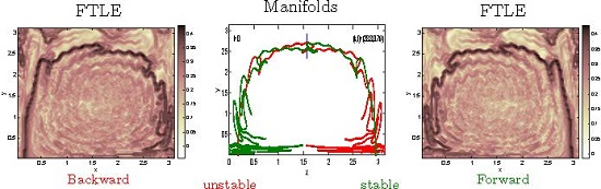
How well do the theoretical flux considerations obtained from Figure 5 match what actually happens? To analyse this, the stable and unstable manifolds for the disturbed system will be used. These are the organizing entities of the chaotic region, and their intersection pattern governs how complicated the mixing is. Figure 7 shows the numerically computed stable and unstable manifolds associated with four different values of the wavenumbers , chosen from Figure 5 and Figure 6 to have tiny, moderate, large and enormous flux amplitudes. Obtaining the manifolds numerically is non-trivial in this case since they are associated with a time-varying anchoring trajectory as opposed to a fixed point, and requires utilizing recent theoretical results [40,41]; a discussion of how these were obtained is given in Appendix C. Figure 7 captures the numerically obtained manifolds only up to a some finite length. All figures are produced by using , a very small perturbation, and the value associated with each pair is given in the captions. In (a), the manifolds fall virtually on top of each other; the interweaving is barely visible. Examining Figure 5, these correspond to wavenumbers in which the amplitude is very close to zero. In (b), there is a mildly discernible difference between the two curves, and in (c), the lobe structure as anticipated by classical results [49,51] and sketched in Figure 2a—but more irregular—is visible. Notice that the expectations of the lobes’ stretching and folding are in fact realized, and so chaotic transport will occur. Even for small ε, there is considerable mixing between the eddy and the jet. This lobe structure is also present in (a) and (b), but the deviations are too small to notice well.
A regime corresponding to a very dark patch in Figure 5, i.e., wavenumbers that our theory tell us correspond to very large transport, is examined in (d). Each manifold starts wiggling considerably when proceeding no great distance from its anchoring trajectory, resulting in a region of complicated intersections. It is worth noting that this intersection pattern does not conform to the “classical” expectation of being like Figure 2a; there are many more wiggles, some lobe structures are very thin, and there are secondary intersections between the stable and unstable manifold. The strong folding (with each manifold folding back on itself at some times) actually causes considerable additional mixing than that addressed here, since thin filaments are more susceptible to destruction via diffusion. There are several reasons for (d) not having the classically expected sinusoidal interweaving between the two manifolds. First, the expectation of the intersection pattern being sinusoidal along Γ is when higher-order terms have been disregarded. In this case, evidently, higher order terms become important. The reason for this is that is so large here that fluid parcels experience large excursions away from the previous eddy/jet boundary, and therefore, their motion is impacted by velocities that are quite far from Γ (it should be noted that the fact that particle excursions are large in no way invalidates the assumption that the velocity disturbance in (13) is small. indeed, since the system is highly chaotic, large particle deviations are to be expected under small velocity disturbances). It is known [52] that even in the time-periodic situation, the lobes created need not always have equal areas, as is apparent in (d). If, however, a much smaller ε were chosen, the excursions would be less, and the more well-behaved structure of (c) would be visible. However, the numerical calculations for (d) were also considerably more difficult than in the others, indicative of the strong chaotic mixing occurring within this manifold intersection region. In this highly chaotic situation, despite small values of ε, the transport between the eddy and jet is large. In any case, since large indicates large excursions, using as a measure of how much fluid/tracer is transported does remain legitimate.
At any frozen time (such as at the time which is pictured), the instantaneous flux is obtainable by (16). The gate is shown by the blue line in all of these panels, and as time progresses forward, say, all curves will “flow to the right” resulting in the intersection patterns moving through the gate. The intersection patterns remains topologically preserved, but the actual shapes of the lobes can change during this procedure. After a time-period of , a picture identical to Figure 7 will emerge, with the lobes having “flowed rightwards” and now being exactly on top of one of the other lobes.
A further validation of these results is presented in Figure 8, which uses Finite-Time Lyapunov Exponent (FTLE) calculations. As argued by Samelson [12], from a practitioner’s viewpoint, the FTLE can be thought of as the Finite-Time Lagrangian Strain (FTLS) incurred by a fluid element located at at a specified time t, under the influence of the flow from time t to (for forward FTLEs) or to for backward FTLEs. Balasuriya et al. [32] rephrase Samelson’s FTLS nomenclature as the Finite-Time Lagrangian Stretching experienced by a circular fluid parcel positioned at each location, after its Lagrangian evolution according to the flow over the specified time interval. Figure 8 shows the forward and backward FTLEs for several of the situations pictured in Figure 7. Under some non degeneracy conditions [32], a strong ridge of the forward FTLE field is a proxy for the unstable manifold, while such a ridge for the backward FTLE is an indicator of the stable manifold [32,54,71]. The FTLE field will change according to the choice of T (the time of flow), for example picking up longer segments of the manifolds for larger T. The “strongest” ridges (black curves) do fall on the stable/unstable manifolds as numerically obtained in Figure 7c,d. This is visible if, for example, comparing the green curve emanating from in Figure 7c with the ridge in Figure 8a; the details of the behavior are spot on. This is also so for the other curves. The much more jagged form of the ridge in Figure 8c,d in comparison with (a) and (b) provides an FTLE justification of greater transport between the eddy and the jet, once again validating the insight gained from Figure 5 on optimal wavenumbers.
FTLE computations (not shown) were also performed for situations in which , when the flux function, and thus the distance between the stable and unstable manifolds on the gate surface, should be zero at all times. The stable and unstable manifolds were seen to line up exactly on top of one another for this choice of disturbance wavenumbers.
Next, the sensitivity of the flux amplitude to the parameters of the main Rossby wave, given for all previous calculations by (37), is examined in Figure 9. These pictures are to be compared with Figure 5. In all cases, only one of the parameters in (37) is changed, with the other three being kept at the fixed values given in (37). The changes considered correspond respectively to a more poleward jet, the zonal jet speed halving, the zonal meanders having a spatial scale which is halved, and the meridional meander extent doubling. The maximum amplitude, as indicated by the colour bars on the left of each figure, does not change much. However, there are significant changes in the locations and distributions of the extrema. In (a) and (c), each zigzag structure of Figure 5 appears to have split apart into two distinct structures. Thus, for example, for eddy/jets further from the equator, it seems that there are many more values of that locally maximize the flux, and that these have flux amplitudes that are not too different from each other. In (b) and (d), the maxima are more diffuse, indicating that if remaining within the (now larger) darker or lighter areas, changing will not lead to much change. In other words, there is less sensitivity to . For example in (d), in which the meridional extent of the meanders is double that for Figure 5, there are very large areas in wavenumber space in which the flux is essentially zero. Therefore, the geometry, location and speed of the meandering jet impacts the amplitude map in non-trivial ways.
The ability to compute pictures such as Figure 9 quickly (each required just a couple of minutes of computation on a laptop computer) makes this a valuable tool. The alternative would be to search the parameter space while for each wavenumber computing a flux-indicator (such as an FTLE field, stable/unstable manifolds, a mix-norm [72] or effective diffusivity [73,74,75] after simulating an advection-diffusion equation). This is numerically prohibitive, and would certainly not enable zeroing in to optimal wavenumbers in the way that Figure 5, Figure 6 and Figure 9 do. As such, the methodology here provides a powerful new tool for seeking the most effective zonal and meridional wavenumbers for mixing.
3.3. Flux for Wave Packets
The flux formulation presented here has the advantage of not requiring time-periodicity. Therefore, it is able to deal with disturbance stream functions consisting not just of one mode, but infinitely many. That is, disturbances of the form (10) or (12) are fair game.
First, consider (10) which has a discrete set (potentially infinite) of values . Nondimensionalizing each according to (20) results in a set of nondimensional wavenumbers , each with its own nondimensional wave speed . For each of these, the flux function is given by (25), where the ε can be replaced by . Given the linearity of the Melnikov process in obtaining this as detailed in Appendix B, the full flux is therefore simply the linear superposition of all these. That is, for the disturbance stream function (10), the flux is given by
where an appropriate “size” measure could be the -norm
(The s must be chosen so that the above converges, and is small.) The formula for and is exactly as is given in (32) and (33). Given the fact that the wavenumbers need not be commensurate, the flux (38) will in general not be periodic in time.
Figure 10a shows the time-varying flux computed for four wavenumbers
for the choice of s for each of these (respectively) as specified. A complicated, time-aperiodic flux results from this, with transport both into and out of the eddy, with many fluctuations.
Next, consider the stream function (12), consisting of wavenumbers across a continuous spectrum. Once again, the same nondimensionalization as before, and the linearity, helps to write the fluid flux directly as
where
As an illustrative example, consider a disturbance stream function which consists of wavenumbers whose radial distance from is normally distributed, according to
Figure 10b shows the resulting flux, computed using (40) and with the dominant wave parameters exactly as in Section 3.2, for the choice of variance . The presence of a continuous range of wavenumbers has caused the flux to be non-periodic. Such computations for any given distribution of wavenumbers—such as obtained from a Fourier decomposition of actual data, say— is easily accomplished using the Formulas (38) and (40).
4. Discussion and Conclusions
The several simple examples presented here for wave packets are a taster for what is possible using the methodology that has been developed for assessing how Rossby-wave eddies interact with jets. In ongoing work, situations that are inspired by geophysical considerations (for example, Gaussian distributions around a collection of wavenumbers which are highly stable), is being pursued. Such an assessment would not be possible if using the classical approach of Poincaré maps and lobe dynamics, since disturbance stream functions of this nature (and appearing in nature) are inevitably not time-periodic. As such, this paper presents a new theoretical tool that can be utilized for transport associated with Rossby waves in generic situations. For example, it is eminently possible in such situations for the stable and unstable manifolds to break apart such that they do not intersect [37,38,41], resulting in a unidirectional flux from the eddy to the jet (causing the eddy to eventually deplete), or in the opposite direction (feeding the eddy from the jet) (incompressibility is preserved in these situations by the fact that the stable and unstable manifolds move in time, for example by shrinking in towards the eddy centre if the eddy is depleting). Many further investigations in this regard are possible, and called for, using these methods. For example, if data are available in a geophysical flow, its spatial Fourier transport can be used to identify the -values that are present, e.g., [83] and the transport impact of this into the future might be estimated. Alternatively, if there are known stable wavenumbers, e.g., [70], the methodology could be applied directly to those.
The ability to determine wavenumbers that are associated with the highest (and least) transport without having to numerically advect particles for each particular wavenumber is significant. This information is available directly from easily computable contour plots such as presented in Figure 5. The insight obtained from the contour plot was additionally validated using several other methods: numerical computation of the stable/unstable manifolds, and FTLE fields. Computing amplitude plots related to different jet geometries, locations and speeds (as shown for example in Figure 9) can provide a simple way of immediately viewing flux-maximizing and minimizing zonal and meridional wavenumbers for that particular dominant Rossby wave. This is in lieu of having to blindly perform numerics such as determining FTLEs, advecting (or advecting-diffusing) many particle trajectories under the flow and computing a mixing measure, etc. Since doing any of these for each choice is computationally expensive, determining which s are most effective for transport is not viable using such a process. As has been demonstrated, dramatically different amounts of transport can occur when different -disturbances are considered. A small investment of energy at the right spatial scales can engender very large transport; is it possible to harness this information for geophysical situations? Is there a relationship to the optimal wavenumbers for vorticity stirring power as developed by Barnes and Hartmann [7]? The fact that larger fluxes arise in (suitably chosen) large wavenumbers indicates that certain small-scale disturbances can contribute highly to flux; can this be used as an advantage in analysing unresolved sub-mesoscale effects?
This article has focussed on the stream functions as being governed specifically by Rossby wave dynamics, and for the eddy-jet geometry associated with a dominant Rossby wave. However, the methodology outlined here is adaptable to stream functions subject to different dynamical constraints, and different geometries which are nevertheless associated with an initially coincident stable and unstable manifolds. It turns out that whenever the (size ε) disturbance stream function has time-sinusoidal dependence (whatever its spatial dependence might be), the flux across the nominal flow barrier will generically always take the form as given in (25), viz., . The details of the amplitude, frequency and phase will of course depend specifically on both the dominant and the disturbance stream function. There is an assumption in deriving this result: that the disturbance stream function is small in comparison to the dominant Rossby wave. In other words, linearized PV-conserving dynamics is assumed. What if the flow were governed by different dynamics, without any such assumptions? Even in this case, the definitions for the tracer flux as given more generally by (18) are valid. It is important to note that (18) is non-perturbative, not requiring any particular component of the velocity field to be weak, and therefore the method would be very general. Given particular models for the velocity field and the tracer dynamics, and s in this equation would take different forms. If it is possible to determine the endpoints of the integration domain (which requires knowledge of the unsteady stable and unstable manifolds), then (18) can be evaluated. This might require numerical evaluation, since s might be available from either observational data or numerical simulations associated with particular dynamics. For explicit forms of s in which perturbative analyses are legitimate, the methodology of Appendix B may be co-opted to determine formulas for the flux amplitude that can be used to investigate optimal wavenumbers associated with these different dynamics.
Another interesting aspect emerging from this study is the ability to quantify the potential vorticity (PV) flux between the eddy and the jet using (17), with s being a dynamically-consistent PV. For example, the dimensional PV could be given by (in dimensional coordinates), which evolves actively according to (34) for some specified dynamical form for N (e.g., diffusive decay, friction, curl of wind-forcing, baroclinic effects). The general flux Formula (18) indicates that the coherent-structure to coherent-structure PV flux is instantaneously given by an integral which is impacted by an interaction between velocity shear and the PV gradient. In contrast, global PV-flux is usually defined in terms of a time-averaged covariance between the velocity field and the PV [23,56,63,64,65,66,67]. Can a connection be established? Moreover, the flux in (18) is a local, but time-varying quantity, which presumably contributes to the global view of PV-fluxes as temporally and spatially averaged quantities [23,56,63,64,65,66,67]. The dynamical-systems viewpoint of this article therefore prompts questions on a new approach to PV-flux analysis. These ideas are currently being investigated.
Acknowledgments
This work was partially supported by the Australian Research Council through Grant FT130100484 of the Future Fellowship scheme.
Conflicts of Interest
The author declares no conflict of interest.
Appendix A. Relationship of Flux Definition to Other Methods
The flux definition (16), and in particular the form (25) obtained for the one-mode Rossby wave disturbance, has strong connections with a variety of other methods which are relevant to transport: lobe dynamics, lobe areas, and the width of the chaotic zone. This Appendix discusses these connections, and also outlines why the method—developed by Balasuriya [41,81]—is more general.
Relationship to relative positioning of manifolds at each time: The flux Formula (16), in the situation in which the disturbance is small, has a connection with the width of the chaotic zone. This is because flux occurs when the distance between and is large, and exactly this distance can be thought of as the width of the zone. Moreover, there is a dichotomy: viewing the width as a function of time at a fixed gate location (which is the viewpoint here), is equivalent to thinking of the width as a function of gate location at fixed time [41,51]. The reason for this is that any intersection patterns that exist at a fixed time, will eventually have to move through a fixed gate when time is evolved. To state this more precisely, let ℓ be a signed arc length along Γ, chosen symmetrically such that the northernmost point of Γ, has , and for . Then, the displacement between the stable and the unstable manifold at a location ℓ, at time t, measured in the direction normal to Γ, can be represented by [41,87]
Here, is the time at which a fluid element at at time zero (i.e., ) passes through a point on Γ with arc length parametrization ℓ, if flowing according to the the unperturbed flow (6) (see [41] for more details). The quantity in (A1) is called a Melnikov function [41,49,51,79,80,88], which has been used previously in the geophysical context [37,44,46,47,80]. For the specific single-mode disturbance discussed in Section 3.2, has the form given in (26), and is sinusoidal (it would have general time-dependence under wave packet disturbances). This implies that for , if viewing the stable/unstable manifolds at a fixed time t, there are infinitely many intersections between them because of ’s sinusoidal behavior. Since they occur along Γ which has finite length, these intersection points accumulate towards the left and right endpoints (there are infinitely many of them, approaching these points arbitrarily closely). Moreover, in approaching these points, which means that width increases without bound. The region between adjacent intersections, i.e., lobes, are therefore closely positioned along Γ in these limits, and exhibits stretching in the transverse direction.
Relationship to chaotic transport: The condition is equivalent to that stated for the flux to be nonzero in (25). In this case, is genuinely sinusoidal. This means it has infinitely many zeros. In view of the dichotomy discussed previously, if considering the picture at fixed time, this implies that the stable and unstable manifolds intersect infinitely often. Determining a zero of a Melnikov function in this way is one of the few approaches for proving that a system has chaotic transport, e.g., [46,47]. The focus in these articles was to prove that the system was chaotic, which occurs when the Melnikov function has simple zeros in time-periodic flows. Technically, however, this furnishes a proof of chaos only in the homoclinic instance in which the two anchoring points are the same; in this case each manifold can be established to wrap around the homoclinic loop, intersecting the other manifold infinitely many times, and re-enter a region arbitrarily close to itself once again. This is a crucial ingredient in the proof of the Smale-Birkhoff theorem [79], one of few tools for proving the existence of chaotic transport. Since this situation is of a heteroclinic manifold, with and being different, the Smale-Birkhoff theorem does not directly apply. In practice, though, the fact that the form (26) implies infinitely many intersections between the stable and unstable manifolds usually does result in chaotic transport between the eddy and the jet. This is because the intersection regions between them (the lobes) must stretch without bound when approaching the ends according to (A1), and the confinement of these lobes which is ensured by the fact that the line is invariant for the stream function (21). Thus, stretching and folding do occur in this situation, with intersection regions eventually forced to re-enter areas from which they left.
In the case of time-sinusoidal perturbations, in which the lobe-dynamics approach is valid, the lobes “move through’ the gate region as time evolves. This results in the flux Function (16) itself being time-sinusoidal; indeed, more can be said [39,81]. There would then be a pulsation of fluid into and subsequently out of, the eddy, during one cycle (corresponding exactly to the sine function being positive over the first half-cycle and negative over the next half-cycle), with this process repeating periodically. For the sakeof argument, suppose that the first half-cycle of this process is like Figure 3a, with fluid passing from the eddy to the jet. One can think of the fluid passing through as “filling a balloon”, with the process stopping when the flux becomes zero, i.e., Figure 3b. The fluid that has “filled the balloon” that has now passed from the eddy to the jet, consists of a fluid area that is exactly the area of the lobe if a lobe-dynamics viewpoint is adopted. During the second half of the cycle, the flux would be in the opposite direction, as pictured in Figure 3c. In this duration, fluid fills out a lobe (which closes off when the stable and unstable manifolds once again meet exactly on the gate, at the end of the second half-cycle of this process) which intrudes from the jet to the eddy. This too has the same area. Thus, during one cycle, a lobe of fluid will go from the eddy to the jet, and another lobe (of the same area) will go from the jet to the eddy. This corresponds exactly to the two lobes that cross the pseudoseparatrix if using the classical lobe dynamics and turnstile approach [49,51], and they are exactly the two lobes lying between and in Figure 2a. Now, in this case, quite much more happens: these lobes travel down towards the anchoring trajectory, which is wobbling around , experiencing elongation in the direction of the opposite manifolds emanating along the line . Since also confined to be above this constant latitude, these lobes inside the eddy fold once they have elongated sufficiently to be once again in the zone of influence of the other anchoring trajectory. The “stretching and folding” as they traverse the boundary region between the eddy and the jet leads to chaotic mixing. This is the fundamental mechanism that creates the well-known chaotic mixing between the eddy and the jet due to time-sinusoidal perturbations [49,51], whose inception is quantified by the flux (16).
Relationship to lobe areas: If , the amplitude has a relationship to the lobes generated when viewing the perturbed system in terms of a Poincaré map in the standard approach. If is time-sinusoidal, these lobes have equal areas, and the area of each lobe can be obtained by integrating the flux function between adjacent zeros [39,52], which in this case gives
Lobe areas typically increase with smaller k due to the presence of the k in the denominator of (A2); the implied conclusion might initially be that transport always increases with decreasing wavenumber. This is a spurious, since there is a time-scale associated with the transport of a lobe. If using the turnstile approach to transport, one lobe will be transported from the eddy to the jet, while another (equally sized) lobe of fluid will transport in the opposite direction from the jet to the eddy, during one iteration of the Poincaré map [49,51]. Since the Poincaré map has period , the average flux (lobe area divided by ) is more appropriate [50]. Examining (A2), this is simply proportional to .
Different gate location: What if the gate were chosen at a different location? In this case, it can be shown [39,41] that the leading-order flux function simply acquires a translation. In other words, this can be accomodateded by a shift in the value of the phase . Importantly, this has no bearing on the amplitude .
A measure of fluid flux: In view of the above discussion, the amplitude of the flux function, is proposed as an appropriate quantifier of the time-varying flux. This makes sense from (26), with the added observation that it is independent of the location at which the gate was positioned. Moreover, it arises naturally from the concept of the average flux, while explicitly accounting for the time-variation in a sensible way. Thus, is an excellent flux measure, consistent with either the lobe dynamics and average flux approach, or the continuous-time approach used here, if .
What if ? Then, the disturbance has no unsteadiness, and so an initial conclusion that can be reached is that flux function is independent of time. If it is a non-zero constant, this means that the stable and unstable manifolds do not intersect. This would allow for a channel to open up, and uni-directional flux will occur between the eddy and the jet (in one direction, depending on this sign of this constant). Uni-directional flux can certainly happen in incompressible geophysically-relevant flows, e.g., Kelvin-Stuart cats-eye flows [37,41], or in kinematical eddies [38], but in these situations there is dissipation due to diffusion or viscosity, and hence the flow is unsteady. This allows for incompressibility to be preserved in the system despite the uni-directional leaking of fluid (from inside the eddy, say), by the stable/unstable manifolds which bound the eddy getting closer and thereby enclosing lesser area as time progresses. In the case examined in this article under the condition , however, the full flow is also steady, and therefore having such a channel open up would violate incompressibility. Therefore, if , the fluid flux must be zero; that is, the stable and unstable manifolds, which may move from their initial locations, do so in such a fashion as to still coincide. This is the reason why the flux is stated as being zero in (25) when the disturbance wavenumbers obey .
Time-periodicity is not necessary: The theoretical approach due to Rom-Kedar et al. [49] was the first to provide a method for quantifying a flux in unsteady flows, due to the intersection of stable and unstable manifolds. This, however, relies on the velocity field being time-periodic, which allows for the definition of a Poincaré map P which simply strobes the flow at the period of the velocity [49,51,79]. Fixed points of P, and their stable and unstable manifolds, are then the focus. Their intersections creates lobes, and the impact of P on these lobes (i.e., the idea of lobe dynamics) gives insight into transport occurring over each time-period. In their classical picture, Rom-Kedar et al. [49] show that the area of a lobe can be used as a transport measure, and in their case the lobes all have equal areas to make this unambiguous. Considerably more details on this are available in the book by Wiggins [51], and geophysical applications are plentiful [3,20,45,46,47,53,80].
The approach discussed in Section 2.2 generalizes this to general time-variation, as will be necessary for Rossby wave packets. There is then no preferred time period to sample the flow at, denying the opportunity of using a map P. One might try to use different Ps for different times or examine quasiperiodic flows to attempt to retain these ideas [57,59], but having a genuinely time-varying approach would be more powerful. Thus, instead of thinking of fixed points of a map, the points to which stable and unstable manifolds are anchored will be thought of in a time-varying way. Therefore, is a time-varying entity to which is attached a stable manifold. It turns out that —previously referred to loosely as a specialized or anchoring trajectory—needs to be defined as a hyperbolic trajectory, which is associated with the concept of an exponential dichotomy [41,89]. This is difficult to use in general to find hyperbolic trajectories, though techniques that work under some circumstances exist [87,90]. However, the point is that a flux, as a genuinely time-varying entity that encapsulates the amount of fluid transferred per unit time, is the most reasonable thing to define.
Lobes are not necessary: The classical approach [49,51] requires there to be lobes present, created through intersecting stable and unstable manifolds. Moreover, to use a lobe area as a measure of transport, it is necessary that these lobes have equal areas. In contrast, the time-varying approach detailed in Section 2.2 does not require the stable and unstable manifolds to intersect at all. If they do not intersect—which is a distinct possibility when including the effects of dissipation in geophysical flows [37,38,41])—there are no lobes at all, and hence no “lobe dynamics”. On the other hand, a lack of intersection makes perfect sense from the perspective of Figure 3: this implies a uni-directional flux, either from the eddy to the jet, or from the jet to the eddy. The instantaneous flux may change with time, but its sign does not.
It is also possible that there are a finite number of intersections between the stable and the unstable manifold. If so, how is lobe dynamics to be thought of? Which lobes get transferred? At what time? Again, the time-continuous approach completely avoids these difficulties.
Compressibility: The flux definition (16) is still legitimate even if the fluid were compressible. The issue is that if the fluid were compressible there would no longer be a stream function ψ that describes the velocity; however, the flux definition remains legitimate with the (compressible) velocity inserted instead [41]. Thus, the only change that needs to be done is the replacement of with the zonal velocity, whatever it happens to be. However, its usage in the compressible case requires a generalization of the standard Melnikov function [41,87].
The Melnikov function and flux: A pleasing theoretical issue of the instantaneous flux was developed by Balasuriya [39,81]: this flux, as a time-varying quantity that specifically measures the amount of fluid that is transported across per unit time, can be characterized to leading-order in ε exactly by the Melnikov function (for fluid applications, see [38,44,46,47,49], for theory, see [41,51,79,88]). The argument of the Melnikov function relates precisely to time, and it is precisely this that appears in (25) and (26). Thus, unlike in the quantification of lobe areas which requires an integral of the Melnikov function [49,50,51], the Melnikov function by itself can be used to quantify the flux as a function of time [39,81]. The quantity presented in this article is exactly such a Melnikov function, as are the expressions (38) and (40) for non-sinusoidal situations. This works under general time-dependence and also compressibility [41].
Appendix B. Derivation of the Formula for A kl
There exists a nice formula for the amplitude of the Melnikov function , using Fourier transforms [41,52], but this requires knowing the formula for the fluid trajectory along Γ according to the flow (6) which went through at time . This can only be defined implicitly, so an alternative will be used.
The formula for in (26) is based on the development outlined by Balasuriya [39,41], building also on prior results [81,87]. It first requires information on how a fluid parcel would flow on the unperturbed flow barrier, Γ, visible in Figure 1. This corresponds to a contour , and so its coordinates obey
where it is recalled that . Thus the x-coordinate on Γ can be written
The x-coordinate of the saddle point on the east is therefore obtained by taking the limit , yielding , and similarly the western saddle point has x-coordinate . The northernmost point on Γ, from (A3), then must satisfy (28). Now, from (6), if ,
where the positive root is chosen since . Set when . Then the time-variation along Γ as a function of y is must be given by
Consider a point with (signed) arc length parametrization ℓ on Γ, chosen such that at . Then, from Equation (19) in Theorem 3 in Balasuriya [39], the width (measured from the stable to the unstable manifold, in the direction of at a location ℓ on Γ), can be represented by
where
Here, is the perturbing velocity, is the unit normal vector to Γ obtained by rotating the velocity vector by in the counter-clockwise direction, and is the time- value, as in (A4), at each location. Equation (A5) represents a signed width, positive if the vector from the stable to the unstable manifold drawn at ℓ is in the same direction as and negative otherwise. Under the definition
can be replaced by in (A5), thereby arriving at (A1). Next, the fluid flux associated with positioning a gate at is given by
where the first equality is because the speed at for the unperturbed flow is , and thus, all points in its vicinity—in particular on the gate—get modified by a term when the disturbance is included. Therefore, (25) has been derived.
The next step is to work with the expression (A6) and to obtain the much more straightforward characterization (26). The disturbance velocity is, from (13) and (22),
Given the different expressions for and on Γ, it helps to think of Γ as consisting of and in these respective domains, and to use the corresponding splitting . On , the normal vector in the direction of is
using (A3). Thus the appropriate unit vector, pointing in this case from inside to outside the eddy, is
Thus,
where the shorthand
for a quantity that depends on both x (which itself depends on y via (A3)) and time t, is used. However, to use (A6), integration with respect to the arc length parameter ℓ is needed. On , the differential elements are related via
where (A3) has been used in simplifying. Therefore
Combining all this information together, this means that the integral on can be written as an integral in terms of y as
where
has both y and t dependence. A similar analysis, whose details will be skipped, enables the expression
where
The function is the sum of and , which can be written alternatively as
where
and
Using standard trigonometric addition formulas on the terms, a sine (respectively cosine) of the quantity appears in each of and , and since independent of y, can be extracted from the integral. This enables , the sum of these two, to be written (using the definitions of and in (30) and (31)) as
using the definitions (32) and (33). This completes the derivation of the sinusoidal flux expression.
Appendix C. Numerical Scheme for Obtaining Stable and Unstable Manifolds
There are many schemes available for numerically computing stable and unstable manifolds for steady flows, since in this case they are attached to an entity (e.g., a fixed point) which does not vary with time. This allows the scheme to start nearby (in some appropriately chosen way) of this exactly known entity. In this case, however, the stable and unstable manifolds are attached to hyperbolic (anchoring) trajectories which are varying with time, and whose location is not explicitly known. To deal with this difficulty, recent developments to approximate the hyperbolic trajectory’s location [87,90] and the direction of emanation of stable/unstable manifolds [40,41] will be used to advantage. Note that hyperbolic trajectory locations are not in general given by instantaneous stagnation points (see examples by [41]), necessitating a more refined approach. The method outlined here is a simple implementation of a broader methodology detailed in Balasuriya [91].
Using Theorem 2.10 in [87], Theorem 2.1 in [40] or Equation (2.5) in [90], the leading-order in ε location of the western (left) hyperbolic trajectory is representable as
(The details of the algebra shall be skipped for brevity.) Similarly, the eastern hyperbolic trajectory is located approximately at
The unstable manifold emanating from when (with no disturbance) points directly northward locally at the hyperbolic trajectory, which in this case is the fixed saddle point . The disturbance would in general give this northward emanation a time-dependent -variation, which is characterized by Theorem 2.2 in [40]. Using this, it turns out (calculations not shown) that the change to this direction is zero. Thus, the unstable manifold, to leading-order in ε, will continue to emanate in the northward direction from the (time-varying) hyperbolic trajectory . Similarly, the stable manifold emanating from will also continue to be in the northward direction locally at .
Armed with this information, a numerical scheme can be devised for determining the unstable manifold attached to , and the stable manifold attached to , at any time t. Let T be a time-of-flow, and δ be a small parameter. To find the unstable manifold emanating from , a line of particles emanating in the northward direction from up to a northward coordinate of δ is seeded. This is an approximation for the local unstable manifold at this instance in time, since the unstable manifold is known to point northwards to leading-order in ε. These particles are then advected forward by one-time step (i.e., to time ) according to (13) with the stream function (22), using a third-order Runge-Kutta scheme. At this next time-step, another line of particles, emanating northward from to a distance δ, is seeded. This is because this is the approximation for the local unstable manifold at this instance in time, which is different from what it was at time . Then, all these particles are advected forward one more time-step, another line of particles is seeded at the new approximate location for the local unstable manifold, etc. This process is continued until the advection has progressed to time t. The particle locations will trace out the unstable manifold at time t. It is necessary to carefully choose how many particles to release at each time step to make sure that in the final result the points trace out the unstable manifold curve to the resolution required, while at the same time not unnecessarily oversampling the unstable manifold curve. Oversampling can be a problem in that, since particles are introduced at every time step, their number can get astronomically large. The release of particles needs to be non-uniform over the time-steps. The sensitivity to the parameters δ and need to also be checked before declaring satisfaction with the results. The parameter T determines how far to extend the unstable manifold.
Similarly, to find the stable manifold emanating from , a line of particles is seeded from northwards to a distance of δ. The advection now occurs in the backward-time direction, but the details of the process are otherwise exactly as for the unstable manifold. Performing these numerical calculations leads to Figure 7.
References
- Randall, D. An Introduction to the Global Circulation of the Atmosphere; Princeton University Press: Princeton, NJ, USA, 2015. [Google Scholar]
- Pedlosky, J. Geophysical Fluids Dynamics; Springer: New York, NY, USA, 1979. [Google Scholar]
- Pierrehumbert, R. Chaotic mixing of tracer and vorticity by modulated travelling Rossby waves. Geophys. Astrophys. Fluid Dyn. 1991, 58, 285–319. [Google Scholar] [CrossRef]
- Mizuta, G. Role of Rossby waves in the broadening of an eastward jet. J. Phys. Oceanogr. 2012, 42, 476–494. [Google Scholar] [CrossRef]
- Graef, F. Free and forced Rossby normal modes in a rectangular gulf of arbitrary orientation. Dyn. Atmos. Oceans 2016, 75, 46–57. [Google Scholar] [CrossRef]
- Kiladis, G. Observations of Rossby waves linked to convection over the eastern tropical Pacific. J. Atmos. Sci. 1998, 55, 321–339. [Google Scholar] [CrossRef]
- Barnes, E.; Hartmann, D. Rossby wave scales, propagation, and variability of eddy-driven jets. J. Atmos. Sci. 2011, 68, 2893–2908. [Google Scholar] [CrossRef]
- Oruba, L.; Lapeyre, G.; Riviere, G. On the northward motion of mid-latitude cyclones in a barotropic meadering jet. J. Atmos. Sci. 2012, 69, 1793–1810. [Google Scholar] [CrossRef]
- Oruba, L.; Lapeyre, G.; Riviere, G. On the poleward motion of mid-latitude cyclones in a baroclinic meandering jet. J. Atmos. Sci. 2013, 70, 2629–2649. [Google Scholar] [CrossRef]
- O’Rourke, A.; Vallis, G. Jet interaction and the influence of a minimum phase speed bound on the propagation of eddies. J. Atmos. Sci. 2013, 70, 2614–2628. [Google Scholar] [CrossRef]
- Haller, G. Lagrangian Coherent Structures. Ann. Rev. Fluid Mech. 2015, 47, 137–162. [Google Scholar] [CrossRef]
- Samelson, R. Lagrangian motion, coherent structures, and lines of persistent material strain. Ann. Rev. Mar. Sci. 2013, 5, 137–163. [Google Scholar] [CrossRef] [PubMed]
- Rypina, I.; Pratt, L.; Pullen, J.; Levin, J.; Gordon, A. Chaotic advection in an archipelago. J. Phys. Oceanogr. 2010, 40, 1988–2006. [Google Scholar] [CrossRef]
- Tew Kai, E.; Rossi, V.; Sudre, J.; Weirmerskirch, H.; Lopez, C.; Hernandez-Garcia, E.; Marsac, F.; Garcon, V. Top marine predators track Lagrangian coherent structures. Proc. Nat. Acad. Sci. USA 2009, 106, 8245–8250. [Google Scholar] [CrossRef] [PubMed] [Green Version]
- Levy, M.; Jahn, O.; Dutkiewicz, S.; Follows, M.; d’Ovidio, F. The dynamical landscape of marine phytoplankton diversity. J. R. Soc. Interface 2015, 12, 20150481. [Google Scholar] [CrossRef] [PubMed]
- BozorgMagham, A.; Ross, S.; Schmale, D. Local finite-time Lyapunov exponent, local sampling and probabilistic source and destination regions. Nonlinear Proc. Geophys. 2015, 22, 663–677. [Google Scholar] [CrossRef]
- d’Ovidio, F.; Fernandez, V.; Hernandez-Garcia, E.; Lopez, C. Mixing structures in the Mediterranean sea from finite-size Lyapunov exponents. Geophys. Res. Lett. 2004, 31, L17203. [Google Scholar] [CrossRef]
- d’Ovidio, F.; Isern, J.; López, C.; Hernández-García, C.; García-Ladona, E. Comparison between Eulerian diagnostics and finite-size Lyapunov exponents computed from the altimetry in the Algerian basin. Deep Sea Res. 2009, 56, 15–31. [Google Scholar] [CrossRef]
- Allshouse, M.; Peacock, T. Refining finite-time Lyapunov ridges and the challenges of classifying them. Chaos 2015, 25, 087410. [Google Scholar] [CrossRef] [PubMed]
- Ngan, K.; Shepherd, T. Chaotic mixing and transport in Rossby-wave critical layers. J. Fluid Mech. 1997, 334, 315–351. [Google Scholar] [CrossRef]
- Joseph, B.; Legras, B. Relation between kinematic boundaries, stirring and barriers for the Antarctic polar vortex. J. Atmos. Sci. 2002, 59, 1198–1212. [Google Scholar] [CrossRef]
- Prants, S.; Budyansky, M.; Ponomarev, V.; Uleysky, M. Lagrangian study of transport and mixing in a mesoscale eddy street. Ocean Model. 2011, 38, 114–125. [Google Scholar] [CrossRef]
- Pratt, L.; Barkan, R.; Rypina, I. Scalar flux kinematics. Fluids 2016, in press. [Google Scholar] [CrossRef]
- Rypina, I.; Kamenkovich, I.; Berloff, P.; Pratt, L. Eddy-induced particle dispersion in the near-surface north Atlantic. J. Phys. Oceanogr. 2012, 42, 2206–2227. [Google Scholar] [CrossRef]
- Mezić, I.; Loire, S.; Fonoberov, V.; Hogan, P. A new mixing diagnostic and Gulf oil spill movement. Science 2010, 330, 486–489. [Google Scholar] [CrossRef] [PubMed]
- Mancho, A.; Small, D.; Wiggins, S.; Ide, K. Computation of stable and unstable manifolds of hyperbolic trajectories in two-dimensional, aperiodically time-dependent vector fields. Physica D 2003, 182, 188–222. [Google Scholar] [CrossRef]
- Haller, G.; Hadjighasem, A.; Farazmand, M.; Huhn, F. Defining coherent vortices objectively from the vorticity. J. Fluid Mech. 2016, 795, 136–173. [Google Scholar] [CrossRef]
- Rypina, I.; Scott, S.; Pratt, L.; Brown, M. Investigating the connection between complexity of isolated trajectories and Lagrangian coherent structures. Nonlinear Proc. Geophys. 2011, 18, 977–987. [Google Scholar] [CrossRef]
- Allshouse, M.; Thiffeault, J.L. Detecting coherent structures using braids. Physica D 2012, 241, 95–105. [Google Scholar] [CrossRef]
- Budis̆ić, M.; Thiffeault, J.L. Finite-time braiding exponents. Chaos 2015, 25, 087407. [Google Scholar] [CrossRef] [PubMed]
- Ma, T.; Bollt, E. Differential geometry perspective of shape coherence and curvature evolution by finite-time nonhyperbolic splitting. SIAM J. Appl. Dyn. Syst. 2014, 13, 1106–1136. [Google Scholar] [CrossRef]
- Balasuriya, S.; Kalampattel, R.; Ouellette, N. Hyperbolic neighborhoods as organizers of finite-time exponential stretching. J. Fluid Mech. 2016. submitted. [Google Scholar]
- Froyland, G.; Horenkamp, C.; Rossi, V.; van Sebille, E. Studying an Agulhas ring’s long-term pathway and decay with finite-time coherent sets. Chaos 2015, 25, 083119. [Google Scholar] [CrossRef] [PubMed]
- Froyland, G.; Stuart, R.; van Sebille, E. How well-connected is the surface of the ocean? Chaos 2014, 24, 0333126. [Google Scholar] [CrossRef] [PubMed]
- Froyland, G.; Padberg, K. Almost-invariant sets and invariant manifolds – connecting probabilistic and geometric descriptions of coherent structures in flows. Physica D 2009, 238, 1507–1523. [Google Scholar] [CrossRef]
- Ser-Giacomi, E.; Rossi, V.; López, C.; Hernández-García, E. Flow networks: A characterization of geophysical fluid transport. Chaos 2015, 25, 036404. [Google Scholar] [CrossRef] [PubMed]
- Balasuriya, S.; Jones, C.; Sandstede, B. Viscous perturbations of vorticity-conserving flows and separatrix splitting. Nonlinearity 1998, 11, 47–77. [Google Scholar] [CrossRef]
- Balasuriya, S.; Jones, C. Diffusive draining and growth of eddies. Nonlinear. Proc. Geophys. 2001, 8, 241–251. [Google Scholar] [CrossRef]
- Balasuriya, S. Nonautonomous flows as open dynamical systems: Characterising escape rates and time-varying boundaries. In Ergodic Theory, Open Dynamics, and Coherent Structures; Bahsoun, W., Bose, C., Froyland, G., Eds.; Springer: Berlin, Germany, 2014; pp. 1–30. [Google Scholar]
- Balasuriya, S. Local stable and unstable manifolds and their control in nonautonomous finite-time flows. J. Nonlinear Sci. 2016, 26, 895–927. [Google Scholar] [CrossRef]
- Balasuriya, S. Melnikov Methods for Flow Barriers and Transport in Unsteady Flows; SIAM Press: Philadelphia, PA, USA, 2016; in press. [Google Scholar]
- Brown, M.; Samelson, R. Particle motion in vorticity-conserving two-dimensional incompressible flows. Phys. Fluids 1994, 6, 2875–2876. [Google Scholar] [CrossRef]
- Balasuriya, S. Gradient evolution for potential vorticity flows. Nonlinear Proc. Geophys. 2001, 8, 253–263. [Google Scholar] [CrossRef]
- Samelson, R. Fluid exchange across a meandering jet. J. Phys. Oceanogr. 1992, 22, 431–442. [Google Scholar] [CrossRef]
- del Castillo Negrete, D.; Morrison, P. Chaotic transport by Rossby waves in shear flow. Phys. Fluids A 1993, 5, 948–965. [Google Scholar] [CrossRef]
- Weiss, J.; Knobloch, E. Mass transport by modulated traveling waves. Phys. Rev. A 1989, 40, 2579–2589. [Google Scholar] [CrossRef]
- Knobloch, E.; Weiss, J. Chaotic advection by modulated traveling waves. Phys. Rev. A 1987, 36, 1522–1524. [Google Scholar] [CrossRef]
- Pratt, L.; Lozier, M.; Beliakova, N. Parcel trajectories in quasigeostrophic jets: Neutral modes. J. Phys. Oceanogr. 1995, 25, 1451–1466. [Google Scholar] [CrossRef]
- Rom-Kedar, V.; Leonard, A.; Wiggins, S. An analytical study of transport, mixing and chaos in an unsteady vortical flow. J. Fluid Mech. 1990, 214, 347–394. [Google Scholar] [CrossRef]
- Rom-Kedar, V.; Poje, A. Universal properties of chaotic transport in the presence of diffusion. Phys. Fluids 1999, 11, 2044–2057. [Google Scholar] [CrossRef]
- Wiggins, S. Chaotic Transport in Dynamical Systems; Springer-Verlag: New York, NY, USA, 1992. [Google Scholar]
- Balasuriya, S. Direct chaotic flux quantification in perturbed planar flows: General time-periodicity. SIAM J. Appl. Dyn. Syst. 2005, 4, 282–311. [Google Scholar] [CrossRef]
- Rypina, I.; Brown, M.; Kocak, H. Transport in an idealized three-gyre system with application to the Adriatic sea. J. Phys. Oceanogr. 2009, 39, 675–690. [Google Scholar] [CrossRef]
- Rypina, I.; Brown, M.; Beron-Vera, F.; Koak, H.; Olascoaga, M.; Udovydchenkov, I. On the Lagrangian dynamics of atmospheric zonal jets and the permeability of the stratospheric polar vortex. J. Atmos. Sci. 2007, 64, 3595–3610. [Google Scholar] [CrossRef]
- Prants, S.; Budyansky, M.; Uleysky, M. Chaotic mixing and transport in a meandering jet flow. Chaos 2006, 16, 033117. [Google Scholar] [CrossRef] [PubMed]
- Miller, P.; Pratt, L.; Helfrich, K.; Jones, C. Chaotic transport of mass and potential vorticity for an island recirculation. J. Phys. Oceanogr. 2002, 32, 80–102. [Google Scholar] [CrossRef]
- Malhotra, N.; Wiggins, S. Geometric structures, lobe dynamics, and Lagrangian transport in flows with aperiodic time-dependence, with applications to Rossby wave flow. J. Nonlinear Sci. 1998, 8, 401–456. [Google Scholar] [CrossRef]
- Mancho, A.; Hernández-Garcia, E.; Small, D.; Wiggins, S.; Fernández, V. Lagrangian transport through an ocean front in the northwestern Mediterranean sea. J. Phys. Oceanogr. 2008, 28, 1222–1237. [Google Scholar] [CrossRef]
- Ide, K.; Wiggins, S. Transport induced by mean-eddy interaction: I. Theory, and relation to Lagrangian lobe dynamics. Commun. Nonlinear Sci. Numer. Simul. 2015, 20, 516–535. [Google Scholar] [CrossRef]
- Kamenkovich, V.; Kamenkovich, I. On the evolution of Rossby waves, generated by wind stress in a closed basin, incoporating total mass conservation. Dyn. Atmos. Oceans 1993, 18, 67–103. [Google Scholar] [CrossRef]
- Peacock, T.; Dabiri, J. Introduction to focus issue: Lagrangian Coherent Structures. Chaos 2010, 20, 017501. [Google Scholar] [CrossRef] [PubMed]
- Peacock, T.; Haller, G. Lagrangian coherent structures: The hidden skeleton of fluid flows. Phys. Today 2013, 66, 41. [Google Scholar] [CrossRef]
- Berloff, P. Dynamically consistent parametrization of mesoscale eddies-Part II eddy fluxes and diffusivity from transient impulses. Fluids 2016, 1, 22. [Google Scholar] [CrossRef]
- Rogerson, A.; Miller, P.; Pratt, L.; Jones, C. Lagrangian motion and fluid exchange in a barotropic meandering jet. J. Phys. Oceanogr. 1999, 29, 2635–2655. [Google Scholar] [CrossRef]
- Shevchencko, I.; Berloff, P. Multi-layer quasi-geostrophic dynamics in eddy-resolving regimes. Ocean Model. 2015, 94, 1–14. [Google Scholar] [CrossRef]
- Maddison, J.; Marshall, D.; Shipton, J. On the dynamical influence of ocean eddy potential vorticity fluxes. Ocean Model. 2015, 92, 169–182. [Google Scholar] [CrossRef]
- Yang, H.; Wu, L.; Shantong, S.; Zhaohui, C. Low-frequency variability of monsoon-driven circulation with application to the South China sea. J. Phys. Oceanogr. 2015, 45, 1632–1650. [Google Scholar] [CrossRef]
- Enomoto, T.; Matsuda, Y. Rossby wavepacket propagation in a zonally-varying basic flow. Tellus 1999, 51A, 588–602. [Google Scholar] [CrossRef]
- Farrell, B. Optimal excitation of neutral Rossby waves. J. Atmos. Sci. 1988, 45, 163–180. [Google Scholar] [CrossRef]
- Balmforth, N.; Piccolo, C. The onset of meandering in a barotropic jet. J. Fluid Mech. 2001, 449, 85–114. [Google Scholar] [CrossRef]
- Shadden, S.; Lekien, F.; Marsden, J. Definition and properties of Lagrangian coherent structures from finite-time Lyapunov exponents in two-dimensional aperiodic flows. Physica D 2005, 212, 271–304. [Google Scholar] [CrossRef]
- Mathew, G.; Mezić, I.; Petzold, L. A multiscale measure for mixing. Physica D 2005, 211, 23–46. [Google Scholar] [CrossRef]
- Nakamura, N. Two-dimensional mixing, edge formation, and permeability diagnosed in area coordinates. J. Atmos. Sci. 1996, 53, 1524–1537. [Google Scholar] [CrossRef]
- Shuckburgh, E.; Haynes, P. Diagnosing transport and mixing using a tracer-based coordinate system. Phys. Fluids 2003, 15, 3342–3357. [Google Scholar] [CrossRef]
- Hendricks, E.; Schubert, W. Transport and mixing in idealized barotropic hurricane-like vortices. Q. J. R. Meteorol. Soc. 2009, 135, 1456–1470. [Google Scholar] [CrossRef]
- Rowe, S.; Hitchman, M. On the relationship between inertial instability, poleward momentum surges, and jet intensifications near mid-latitude cyclones. J. Atmos. Sci. 2016, 73, 2299–2315. [Google Scholar] [CrossRef]
- Held, I.; Pierrehumbert, R.; Garner, S.; Swanson, K. Surface quasi-geostrophic dynamics. J. Fluid Mech. 1995, 282, 1–20. [Google Scholar] [CrossRef]
- Bower, A. A simple kinematic mechanism for mixing fluid across a meandering jet. J. Phys. Oceanogr. 1991, 21, 173–180. [Google Scholar] [CrossRef]
- Guckenheimer, J.; Holmes, P. Nonlinear Oscillations, Dynamical Systems and Bifurcations of Vector Fields; Springer: New York, NY, USA, 1983. [Google Scholar]
- Samelson, R.; Wiggins, S. Lagrangian Transport in Geophysical Jets and Waves; Interdisciplinary Applied Mathematics; Springer: Berlin, Germany, 2006. [Google Scholar]
- Balasuriya, S. Cross-separatrix flux in time-aperiodic and time-impulsive flows. Nonlinearity 2006, 19, 282–311. [Google Scholar] [CrossRef]
- Haller, G.; Poje, A. Finite time transport in aperiodic flows. Physica D 1998, 119, 352–380. [Google Scholar] [CrossRef]
- Chelton, D.; Gaube, P.; Schlax, M.; Early, J.; Samelson, R. The influence of nonlinear mesoscale eddies on oceanic chlorophyll. Science 2011, 334, 328–332. [Google Scholar] [CrossRef] [PubMed]
- Gaultier, L.; Djath, B.; Verron, J.; Brankart, J.M.; Brasseur, P.; Melet, A. Inversion of submesoscale patterns from a high-resolution Solomon Sea model: Feasibility assessment. J. Geophys. Res. Oceans 2014, 119, 4520–4541. [Google Scholar] [CrossRef]
- McIntyre, M. Potential vorticity. In Encyclopedia of Atmospheric Science, 2nd ed.; North, G., Zhang, F., Pyle, J., Eds.; Elsevier: Amsterdam, The Netherlands, 2012. [Google Scholar]
- Hadjighasem, A.; Karrasch, D.; Teramoto, H.; Haller, G. Spectral clustering approach to Lagrangian vortex detection. Phys. Rev. E 2016, 93, 063107. [Google Scholar] [CrossRef] [PubMed]
- Balasuriya, S. A tangential displacement theory for locating perturbed saddles and their manifolds. SIAM J. Appl. Dyn. Syst. 2011, 10, 1100–1126. [Google Scholar] [CrossRef]
- Melnikov, V.K. On the stability of the centre for time-periodic perturbations. Trans. Mosc. Math. Soc. 1963, 12, 1–56. [Google Scholar]
- Coppel, W.A. Dichotomies in Stability Theory; Number 629 in Lecture Notes in Mathematics; Springer-Verlag: Berlin, Germany, 1978. [Google Scholar]
- Balasuriya, S.; Padberg-Gehle, K. Controlling the unsteady analogue of saddle stagnation points. SIAM J. Appl. Math. 2013, 73, 1038–1057. [Google Scholar] [CrossRef]
- Balasuriya, S. A numerical scheme for computing stable and unstable manifolds in nonautonomous flows. Int. J. Bifurc. Chaos 2016. submitted. [Google Scholar]
Figure 1.
One-wave Rossby wave in the moving frame, with , where Γ (magenta curve) is the barrier between the chosen eddy and the jet.
Figure 1.
One-wave Rossby wave in the moving frame, with , where Γ (magenta curve) is the barrier between the chosen eddy and the jet.

Figure 2.
The (a) Poincaré map, and (b) the time-continuous, approaches for the splitting of the eddy-jet barrier into stable (green) and unstable (red) manifolds when . The dashed blue line is Γ, the unambiguous barrier when , and the Poincaré map is valid only under certain conditions, as explained in the text. (a) Discrete (strobing) time; (b) continuous time.

Figure 3.
Intersection possibilities at three instances in time. (a) Positive flux; (b) zero flux; (c) negative flux.
Figure 3.
Intersection possibilities at three instances in time. (a) Positive flux; (b) zero flux; (c) negative flux.

Figure 4.
The instantaneous flux Function (26) for , at several zonal wavenumber values: (blue), 6 (red) and 18 (yellow).
Figure 4.
The instantaneous flux Function (26) for , at several zonal wavenumber values: (blue), 6 (red) and 18 (yellow).

Figure 5.
Dependence of amplitude on the wavenumbers , with the dashed blue curve corresponding to .
Figure 5.
Dependence of amplitude on the wavenumbers , with the dashed blue curve corresponding to .

Figure 6.
Zoom in to smaller wavenumbers in Figure 5.
Figure 6.
Zoom in to smaller wavenumbers in Figure 5.

Figure 7.
Numerically computed stable (green) and unstable (red) manifolds at using and . (a) , ; (b) , ; (c) , ; (d) , .
Figure 7.
Numerically computed stable (green) and unstable (red) manifolds at using and . (a) , ; (b) , ; (c) , ; (d) , .

Figure 8.
Forward and backward FTLE fields at for identical parameter values as in Figure 7c,d, with the choice of flow-time . (a) , forward; (b) , backward; (c) , forward; (d) , backward.
Figure 8.
Forward and backward FTLE fields at for identical parameter values as in Figure 7c,d, with the choice of flow-time . (a) , forward; (b) , backward; (c) , forward; (d) , backward.

Figure 9.
Changes to the flux amplitude when one of the parameters each in (37) is changed, with the the others kept fixed. (a) ; (b) ; (c) ; (d) .
Figure 9.
Changes to the flux amplitude when one of the parameters each in (37) is changed, with the the others kept fixed. (a) ; (b) ; (c) ; (d) .


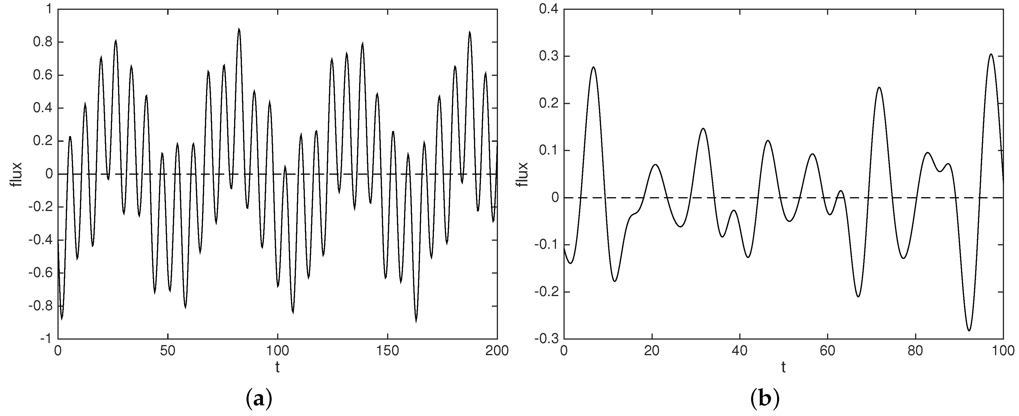
© 2016 by the author; licensee MDPI, Basel, Switzerland. This article is an open access article distributed under the terms and conditions of the Creative Commons Attribution license ( http://creativecommons.org/licenses/by/4.0/).
Share and Cite
MDPI and ACS Style
Balasuriya, S. Meridional and Zonal Wavenumber Dependence in Tracer Flux in Rossby Waves. Fluids 2016, 1, 30. https://doi.org/10.3390/fluids1030030
AMA Style
Balasuriya S. Meridional and Zonal Wavenumber Dependence in Tracer Flux in Rossby Waves. Fluids. 2016; 1(3):30. https://doi.org/10.3390/fluids1030030
Chicago/Turabian StyleBalasuriya, Sanjeeva. 2016. "Meridional and Zonal Wavenumber Dependence in Tracer Flux in Rossby Waves" Fluids 1, no. 3: 30. https://doi.org/10.3390/fluids1030030