1. Introduction
A Venturi flume is a critical-flow flume, wherein the critical depth is created by a local diminution of the channel width. For open channel conveyance systems, the Venturi flume offers the simplicity of a direct correlation between the upstream head and a corresponding discharge. Compared to a weir, this flume possesses the advantages of operating successfully without significant deposition of sediments and conveying water with smaller energy losses [
1]. If the Venturi flume is designed to be operated under free flow conditions, the flow passes from the subcritical to the supercritical state through the flume channel. In a long-throated flume, the prismatic throat section has a sufficient length in the streamwise direction to achieve a nearly parallel flow situation and a hydrostatic pressure distribution (see, e.g., [
2]). Contrary to this, the flow pattern in the control section of a short-throated flume is characterised by a strong free surface curvature and a departure from the hydrostatic distribution of pressure [
3,
4,
5]. In a bottom hump type of such flume, the combined effects of the sidewalls and streamline vertical curvatures predominantly affect the behaviour of the curvilinear flows, especially in the vicinity of the critical section where the flows exhibit three-dimensional (3D) characteristics with cross-waves. In the region downstream of the critical section, the cross-waves influence the configuration of the free surface profile. Furthermore, the pattern of the curvature of the streamlines is influenced by the contraction ratio and the shape of the diverging section [
3]. The detailed description of the flow field of a short-throated flume requires a higher-order numerical model that includes more detailed information in the form of vertical velocity and non-hydrostatic pressure distributions, as well as the effect of the curvature of the sidewalls. Several previous studies focused only on the simulation of curvilinear flows over sills (see, e.g., [
6,
7,
8,
9,
10,
11]). In comparison, detailed numerical investigations have not been systematically carried out for free flows in Venturi flumes with and without bottom humps using a higher-order one-dimensional model. From the practical point of view, an accurate one-dimensional non-hydrostatic model can effectively supplement experimental studies for developing discharge rating curves and studying the hydraulic behaviour of full-scale Venturi flumes.
Modelling of curvilinear free surface flow has been the core part of many research works in the past. A number of investigations have been performed to extend the Saint-Venant equations by considering the vertical curvature of the streamline and its associated effects on the velocity and pressure distributions (see, e.g., [
12,
13,
14]). In addition, Berger and Carey [
6,
7], Dowels et al. [
15] and Anh and Hosoda [
16] extended the Dressler [
17] approach and developed the depth-averaged equations for modelling free surface flows over curved boundaries. However, none of these equations include terms accounting for sidewall curvature and apply only to open channel flows in which the effect of the streamline vertical curvatures is significant. Other investigators [
18] generalised the Fenton [
14] approach and developed a higher-order one-dimensional flow equation that includes implicitly the effect of the channel width variation due to diverging and/or converging vertical sidewalls. However, the application of the equation is limited to the modelling of free surface flows in short-throated flumes with broken plane transition only. Recently, Cheng et al. [
19] extended the Khan [
20] equations, which were developed based on the assumption of linear variations of vertical velocity and non-hydrostatic pressure distributions, for steady flow over a curved bed with sidewall curvatures. However, their method does not permit the effect of the streamwise channel width variation to be incorporated in the vertical velocity profile. Consequently, the pressure equation lacks terms that account for the effect of sidewall curvatures. Furthermore, detailed experimental studies [
21,
22] have shown that the assumption of a linear variation of a non-hydrostatic pressure distribution cannot always be valid, especially for curvilinear open channel flows.
In more recent numerical approaches, the horizontal two-dimensional (2D) shallow-water equations with sources terms have been applied to solve the channel transition (rapid contraction and/or expansion) problems (see, e.g., [
23,
24,
25]). In these approaches, the source terms related to the bed topography and bed shear stress have been discretised using suitable techniques. As highlighted by Berger and Carey [
7] and Shimozono and Sato [
26], the hydrostatic pressure hypothesis severely affects the results of the shallow-water models for flow with substantial curvatures of the streamline.
The aim of the current work is two-fold. First, an alternative higher-order model for open channel flows in short-throated flumes is developed without resorting to any assumptions on the distributions of the vertical velocity and pressure. The horizontal velocity and pressure distribution information are incorporated into the model following the Serre [
27] approximation and Boussinesq’s [
28] approach for the treatment of the vertical acceleration in the streamwise equation of motion. The Serre [
27] simplifying approximation is commonly applied in open channel hydrodynamics particularly for modelling curved flow problems (see, e.g., [
29,
30]). Compared to 2D non-hydrostatic and quasi-3D numerical models, the proposed model is computationally efficient and is simple to apply. Moreover, it is capable of providing a convenient method of developing a rating curve for a critical-flow flume under free flow conditions. The second aim is to explore the capabilities of the model for simulating the important aspects of curvilinear flows in short-throated flumes with and without bottom humps. In the modelling of such a type of complex flow problem, the common practice is to simplify and solve the problem as a 2D flow problem in the vertical plane (see, e.g., [
1,
19]). Accordingly, the free surface profile is simulated by computing the depths along the centreline of the channel using the proposed one-dimensional non-hydrostatic model. This approach enables us to assess the influence of the sidewalls and streamline vertical curvatures on the free surface profile and pressure distribution solutions of the model, as well as on the discharge characteristics of the critical-flow flumes. It is important to note that numerical investigation of sediment-laden flow in a non-prismatic channel is beyond the scope of this study.
The remaining sections of this paper are organised as follows. In the following sections, the derivation of the governing equations is presented first, followed by a brief discussion of the main features of the extended computational model, namely the spatial discretisation of the equations. The solution procedures for the resulting nonlinear discretised equations and the boundary conditions associated with the numerical model are also depicted. A brief discussion of the model results is presented by comparing them with experimental data and earlier numerical results from the literature. The paper is ended with conclusive remarks.
2. Governing Equations
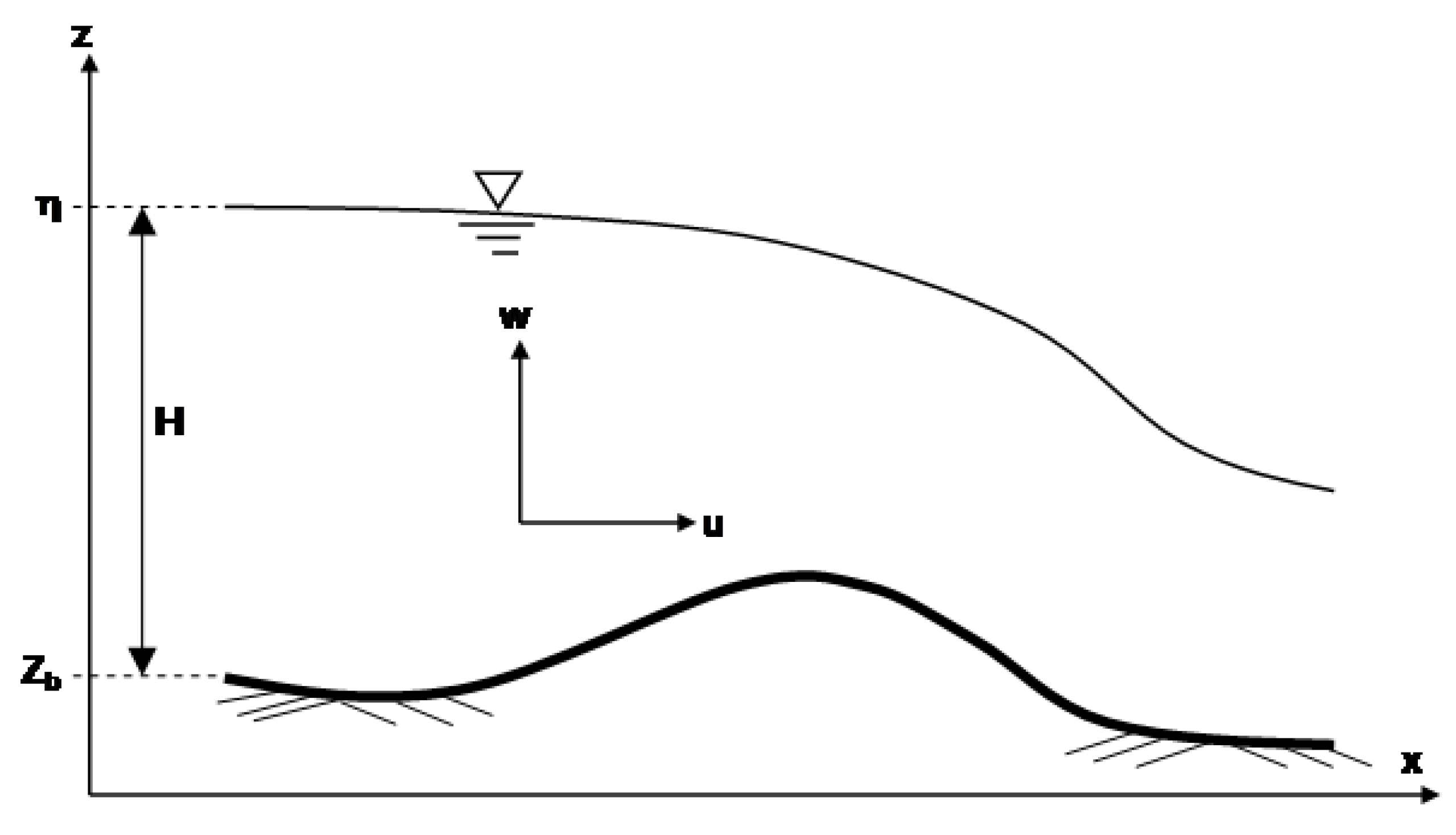
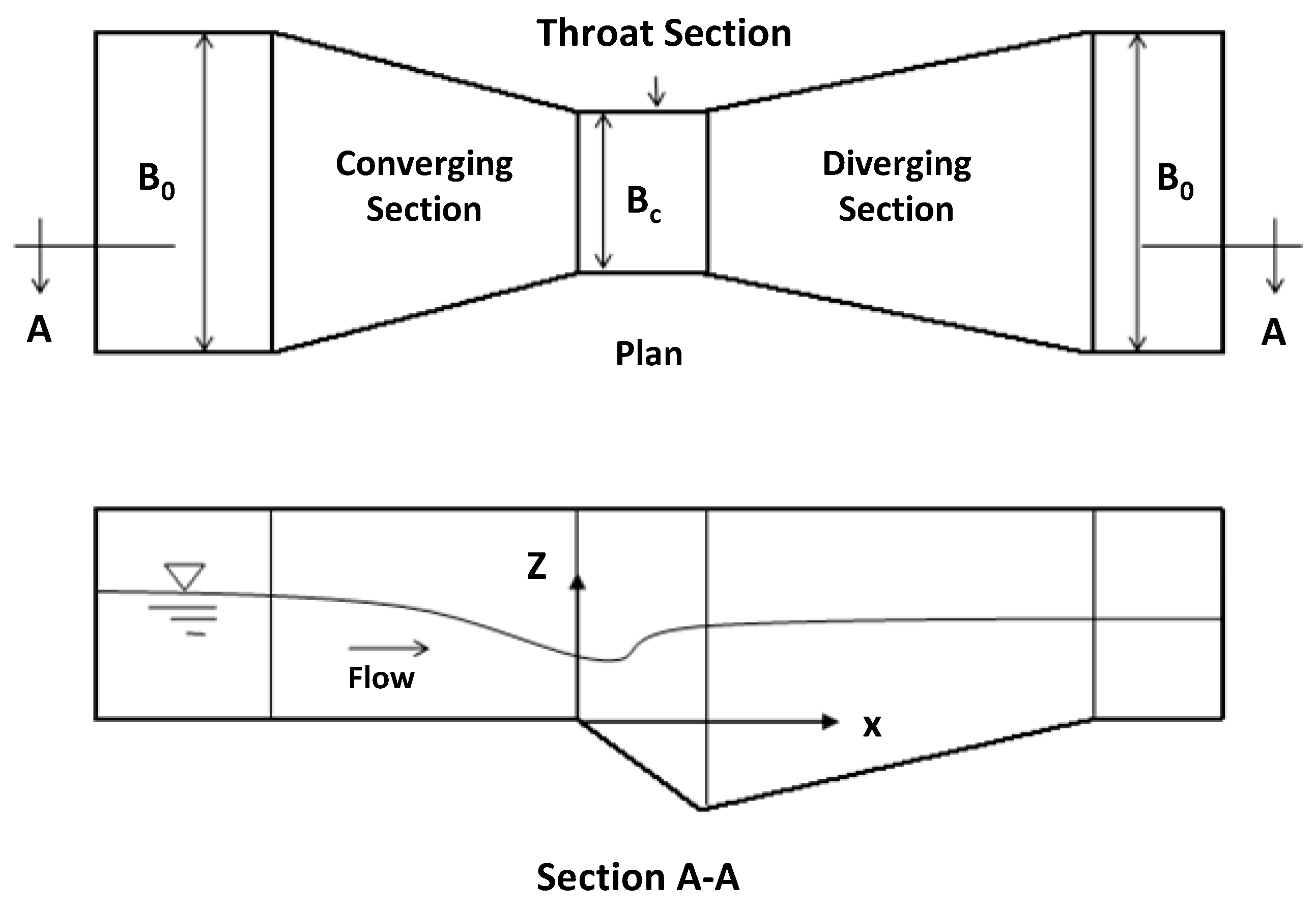
Consider a non-prismatic channel section, and define Cartesian orthogonal coordinates, such that
x is horizontally along the channel,
y is horizontally in the transverse direction and
z is vertically upward.
Figure 1 depicts the notation used. The Fenton [
14] one-dimensional dynamic equation, which was developed based on the consideration of momentum in a control volume, reads as:
where
Sf denotes the friction slope, calculated from Manning’s equation or the smooth boundary resistance law;
is the discharge;
is the flow cross-sectional area;
is the density of the fluid;
is the pressure;
refers to the Boussinesq coefficient;
is gravitational acceleration;
is the contribution of an inflow of
volume rate per unit length, with streamwise velocity component
, and
is the time.
The continuity equation for a 2D open channel flow may be written as:
where
and
are the Cartesian velocity components in the horizontal and vertical directions, respectively. Using the zeroth-order approach, the horizontal velocity profile at a vertical section is approximated by its depth-averaged value as [
27]:
where
is the unit discharge;
B is the channel width; and
H is the depth of flow. Such a rigorous simplifying approximation is not uncommon in open channel hydrodynamics for the curved flow situation (see, e.g., [
31]). Furthermore, the contributions of the transverse velocity components,
, are neglected (
), so that the flow problem can be treated as a 2D problem in the vertical plane.
Substituting Equation (3) in Equation (2) and vertically integrating from
z to
gives an equation for the vertical velocity distribution after employing the kinematic boundary condition,
, at the free surface:
where
is the mean free surface elevation;
is the channel bed elevation;
is the slope of the tangent of the channel bed profile; and
is the vertical velocity at the free surface. Equation (4a) implicitly includes the effect of the breadthwise contraction and/or expansion in the vertical velocity distribution.
In a steady nonuniform open channel flow (
), the pressure distribution in the flow field is obtained from the integration of the Euler equation [
32],
where
is the body force per unit mass and
is the pressure gradient in the vertical direction.
To develop the pressure distribution equation for a curved streamlined flow in a non-prismatic rectangular channel, Equation (4a) is differentiated with respect to
, and then, the resulting equation is inserted into Equation (5). By multiplying this equation throughout by
and vertically integrating from
z to
η, the following equation is obtained:
The right-hand side of this equation consists of the hydrostatic pressure term and terms that account for the dynamic pressure effects. The effects of the dynamic pressure depend on the vertical curvatures of the bed and streamline, and the pressure change brought by the streamwise channel width variation and sidewall curvature. If we compare Equation (6) to the Cheng et al. [
19] pressure equation, we remark that the third and fourth terms of Equation (6) do not appear in Cheng et al.’s [
19] equation. In addition to these two terms, the last term is not included in Fenton and Zerihun’s [
18] model. As discussed before, these higher-order terms take into account the effects of the sidewalls and streamline vertical curvatures and significantly affect the accuracy of the numerical results. If the curvatures of the streamline and the bed are neglected, i.e.,
, this higher-order equation reduces to the well-known hydrostatic pressure equation for flow in a prismatic channel (
). It is noticed that the terms that account for the dynamic effects due to the vertical acceleration of the flow show a quadratic variation in Equation (6). Compared to a linearly varying non-hydrostatic pressure equation, this equation more accurately simulates the pressure distribution of a strongly curved streamlined flow. Substituting
by
and then
by
in Equation (6) gives the following equation for modelling the bed pressure profile:
where
is the bed pressure.
It is also assumed that the free surface is horizontal in the transverse direction, so that the pressure is not a function of
. Using this approximation, the pressure equation, Equation (6), is differentiated with respect to
and then integrated across the channel. After substituting the resulting equation into Equation (1) and eliminating the unsteady terms using the relationships
and
, the following equation for flow in a non-prismatic rectangular channel is obtained:
where
and
are the second and third derivatives of the bed profile, respectively and
is the vertical coordinate of a point in the flow field. Equation (8) is a generalised higher
-order equation for steady rapidly-varied flow problems where the effects of the sidewalls and streamline vertical curvatures are significant. It includes terms due to sidewall curvature that originate from the vertical velocity profile as a result of the breadthwise contraction and/or expansion. This implies that a higher-order correction is incorporated in Equation (8) compared to the correction that was applied to Cheng et al.’s [
19] equation for the effects of the dynamic pressure. In a special case of weakly-curved free surface flow in a prismatic channel, the contributions of the products of the derivatives are insignificant compared to the derivatives themselves. Using this approximation, Equation (8) reduces to an equation structurally similar to the classical Boussinesq-type momentum equation [
28] that was developed based on the assumption of irrotational flow. Nonetheless, the method presented here demonstrates that this assumption is not really required to develop such a type of flow equation.
As described before, the momentum approach has been applied to develop the above governing equations. In this approach, the friction slope term stands for the resistance due to external boundary stresses. Since the current method does not account for the effective stresses arising from turbulence stresses and stresses due to vertical averaging, the friction slope term implicitly accounts for the aggregate losses.
Equations (6) and (8) will be used in this study for modelling the important aspects of steady curvilinear flows in short-throated flumes with and without bottom humps. The numerical solutions of the equations will be compared to measurements and previous numerical results. The results of validating the flow model for such a type of flow problem will provide significant insight into how well the model will perform in complex rapidly-varied flow situations.
Boundary Conditions
The complete numerical solutions of the Venturi flume flow problems using the model equation require the following three external boundary conditions to be specified at the inflow and outflow sections, which are located in the flow region, where the effects of the vertical curvature of the streamline are insignificant.
Inflow Boundary Condition
At the inflow section, the slope of the free surface and the flow depth are imposed as boundary conditions. The quasi-uniform flow condition simplifies the evaluation of the free surface slope,
, at this section using the gradually-varied flow equation,
where
F is the Froude number and
S0 is the bed slope.
Outflow Boundary Condition
At the outflow section, the flow depth is specified as a boundary condition and remained unchanged during the computations.
3. Numerical Solution Procedure
A numerical solution is necessary since an analytical solution that satisfies the specified boundary conditions is not available for this nonlinear flow equation. The numerical model that was developed by Zerihun [
33] for the simulation of flow over curved beds is extended here to handle a Venturi flume flow problem. For the purpose of discretisation, Equation (8) is rewritten in terms of the local flow depth using the relationships,
and is represented by a simple general equation as:
where
and
are the nonlinear coefficients at node
associated with the model equation and are given by:
For minimising the truncation errors due to the approximate formulation of the finite difference expressions, higher-order finite difference formulae are employed to discretise the third-order differential Equation (10b) (see, e.g., [
34]). Hence, the upwind finite difference approximations for the first and third derivative terms and the central difference for the second derivative term [
35] are used to replace the derivative terms of this equation. After simplifying the discretised equation and combining similar terms together, the final equation reads as:
where
is the step size. Since the value of the nodal point at
(inflow section) is known, the value of the imaginary node at
can be determined from the estimated free surface slope,
, at the inflow section. Using the discretised equation of the free surface slope at the inflow section and the expanded form of Equation (12) at
, the following implicit finite difference equation in terms of the nodal values at
, 0 and 1 is obtained:
Equations (12) and (13) are the corresponding finite difference equations for the third-order differential flow equation, which are to be solved numerically by specifying the boundary conditions at the two extreme sections of the solution domain. In general, such a boundary value problem must be solved by an iterative method, which starts from an initial estimate for the free surface position using the Bernoulli and continuity equations. Then, to simulate the free surface profile, Equation (12) is applied at different computational points within the solution domain and results in a sparse system of nonlinear algebraic equations. Equation (13) together with the nonlinear algebraic equations and the two boundary values prescribed at the inflow and outflow sections are solved iteratively by the Newton–Raphson method with the numerically-determined Jacobian matrix. The following criterion based on the correction depths is used to assess the convergence of the solution:
where
is the estimated correction depth at any stage of the iteration process at nodal point
;
is the total number of computational nodes excluding boundary nodes at the inflow and outflow sections; and
is the specified tolerance for the convergence of the numerical solution.
For discretising the derivative term in the pressure equation, a similar finite difference formula is inserted into Equation (6). The discretised equation is then applied to compute the pressure profiles at different sections using the known flow depths from the numerical solution of the flow profile equation.
4. Model Verifications
This section analyses the application of the proposed one-dimensional non-hydrostatic model to various curvilinear free surface flow situations and compares the predictions to experimental data and previous numerical results available in the literature. For the purpose of assessing the effect of the streamwise width variation on the solution of the model, the following test cases related to flows in short-throated flumes with different contraction ratios,
(
= the width of the throat or control section,
= the width of the upstream inlet section), were considered: (i) transcritical flow in a flume with broken plane transition (Parshall flume); (ii) transcritical flow in a horizontal bed short-throated flume with rounded transition; and (iii) curvilinear free surface flow in a channel with a curved sidewall and bed. For all test cases presented here, the experiments were performed in hydraulically-smooth laboratory flumes, which were made of plexiglass. Hence, a smooth boundary resistance method based on the Darcy–Weisbach equation was used to compute the friction slope [
31,
33]. For the purpose of simplifying the computational procedure, β was assumed as unity in the model. Such a simplifying assumption does not significantly affect the accuracy of the numerical solutions [
33].
For all test cases studied, the step size was reduced until there was no substantial change in the numerical solution. Consequently, the final computational results were free of any numerical errors arising from the effect of spatial step size.
In order to evaluate the performance of the model systematically, the relative error between the predicted and measured values is calculated using the following equation:
where
is the relative error and the subscripts
and
denote the computed and measured values of the parameter
, respectively. A satisfactory performance was assumed when the estimated maximum relative error was less than 5%.
4.1. Curvilinear Flow in Short-Throated Flumes
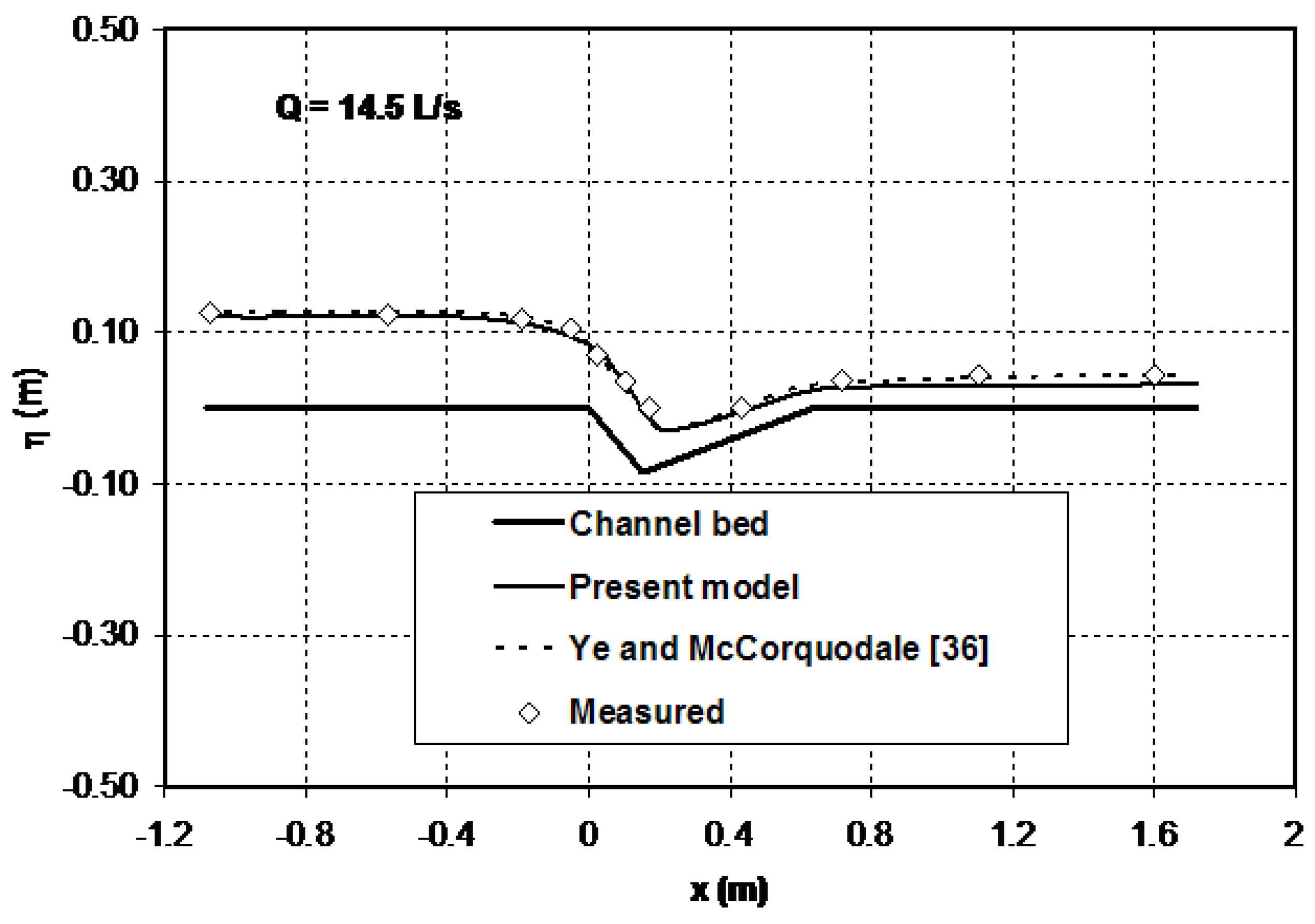
4.1.1. Flow in a Parshall Flume
The free surface profile experimental data from Ye and McCorquodale [
36] are selected for the verification of the model. The experiment was performed in a Parshall flume model that consists of a horizontal bed inlet section with converging sidewalls, a prismatic throat section with a downward sloping bed and an outlet section with diverging sidewalls and an adverse sloping bed (see
Figure 2). The width of the Parshall flume in the converging and diverging sections is computed using the following equations:
where
= 0.3048 m is the width of the channel at the upstream end of the converging section. For this test case, the upstream end of the throat section was considered as the origin of the Cartesian coordinate system.
Figure 3 compares the computational result of the present model for the free surface profile along the centreline of the flume with the laterally-averaged experimental data for transcritical flow in a Parshall flume. The prediction of the present model is also compared in this figure with the previous numerical result obtained by Ye and McCorquodale [
36] using a 2D depth-averaged model. Both numerical models accurately reproduce the free surface profile in the vicinity of the critical section for this test case. In the subcritical flow region, the agreement between the results of the models and the experimental data is remarkable. In general, no appreciable differences are seen between the numerical results of the two models in the flow region upstream of the critical section. However, the result of the present model slightly deviates from measurements (maximum relative error = 2.8%) in the supercritical flow region downstream of the diverging section (
). As a one-dimensional non-hydrostatic model, this model does not capture the pattern of the cross-waves, which usually appear in the region downstream of the throat section.
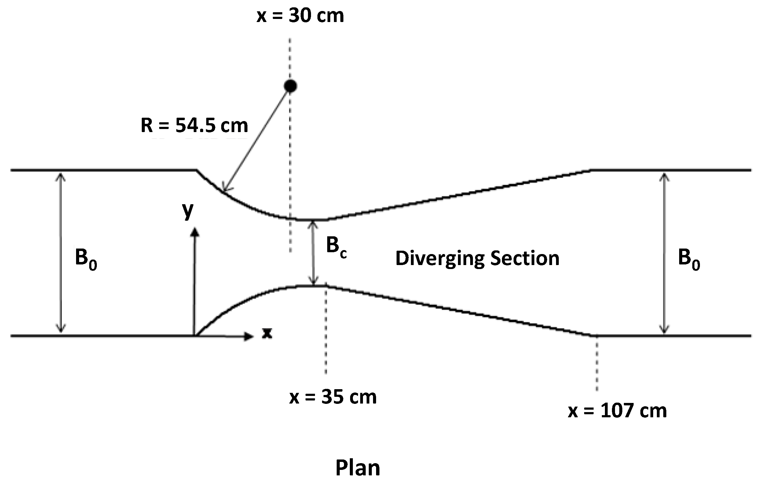
4.1.2. Flow in a Horizontal Bed Flume with Rounded Transition
Khafagi [
37] conducted a series of experiments on free surface flows in a Venturi flume with rounded transition. The horizontal bed test flume consists of a circular-shaped converging section, a short prismatic throat section and a diverging section with an expansion ratio of 1:8, as shown in
Figure 4. The contraction ratio of the flume is 0.40. The width of this flume in the converging and diverging sections is computed by:
where
is the horizontal distance in metres from the start of the converging section and
= 0.545 m is the radius of the channel sidewalls. The test data for free surface and pressure profiles and velocity distributions were used to verify the model. Full details of the experimental set-up and procedures can be found in Khafagi [
37].
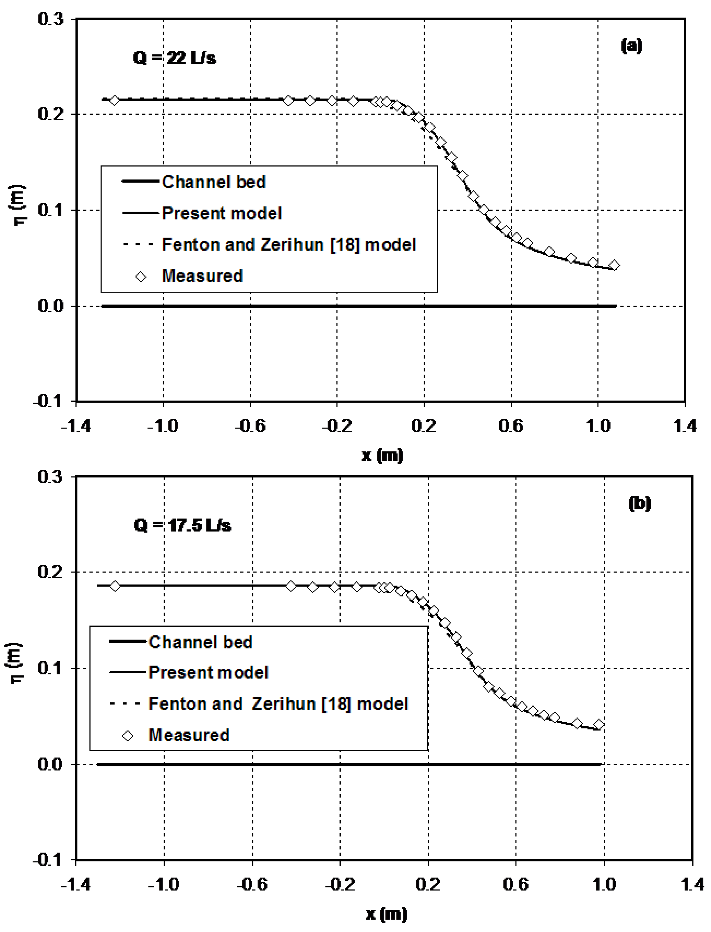
Figure 5 compares the computed free surface profiles using the present model and Fenton and Zerihun’s [
18] Boussinesq-type momentum model with experimental data. As described before, this Boussinesq-type model incorporates a correction only for the effect of the streamwise channel width variation. In the subcritical flow region (
), the numerical results of the two models show excellent agreement with experimental data for the free surface profile. As illustrated in
Figure 5, however, the predictions of the Fenton and Zerihun [
18] model slightly deviate from the measurements (maximum relative error = 3.8%), especially in the converging section of the flume (
). In this section, the sidewall-induced curvature strongly influences the solutions of this model.
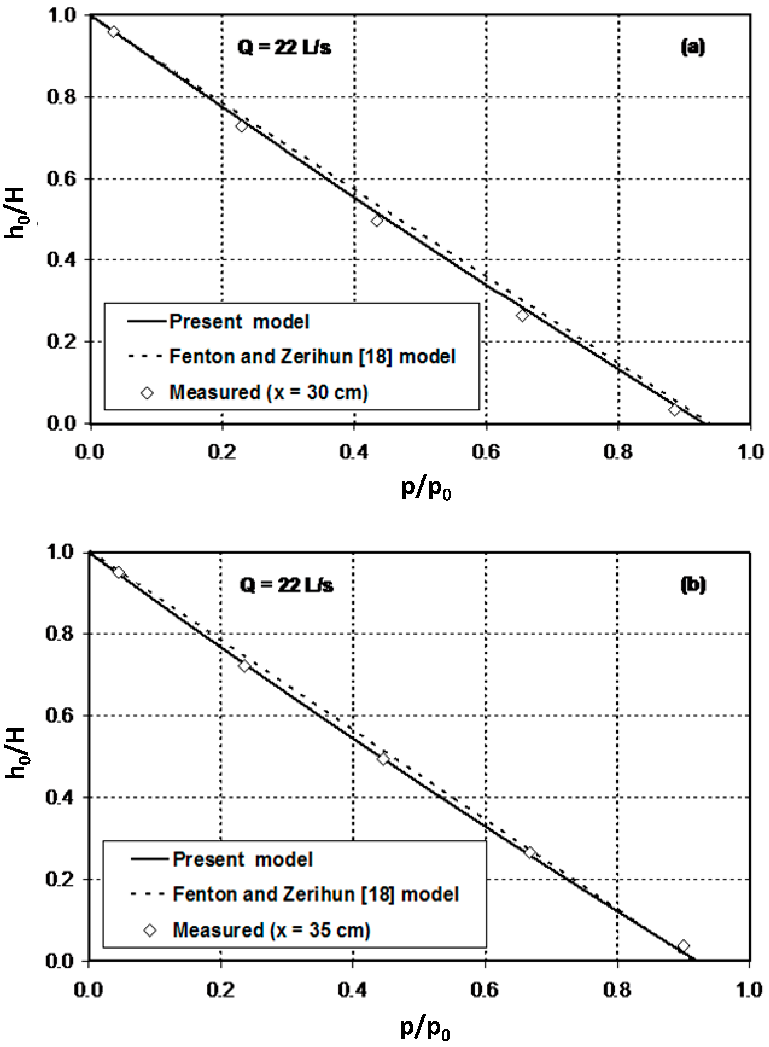
For assessing the impact of the applied corrections for the effects of the sidewalls and streamline vertical curvatures in the simulation results of the model, the vertical distributions of the pressure at the upstream (
) and downstream (
) ends of the throat section are modelled. In this section of the flume, the effect of the curvature of the sidewalls might not be expected to be significant.
Figure 6 compares the computational results of the present model for pressure distributions against the experimental data points. The numerical results of Fenton and Zerihun’s [
18] model are also plotted. In this figure, the variation of the normalised pressure,
(
is the pressure at a vertical distance of
above the bed,
), with the normalised vertical distance above the bed,
, is shown. In both simulation cases, the predictions of the present model compare favourably to the experimental data and show a slight improvement against the predictions of the Fenton and Zerihun [
18] model. The maximum relative errors for the present model and Fenton and Zerihun’s model are only 1.3% and 3.5%, respectively.
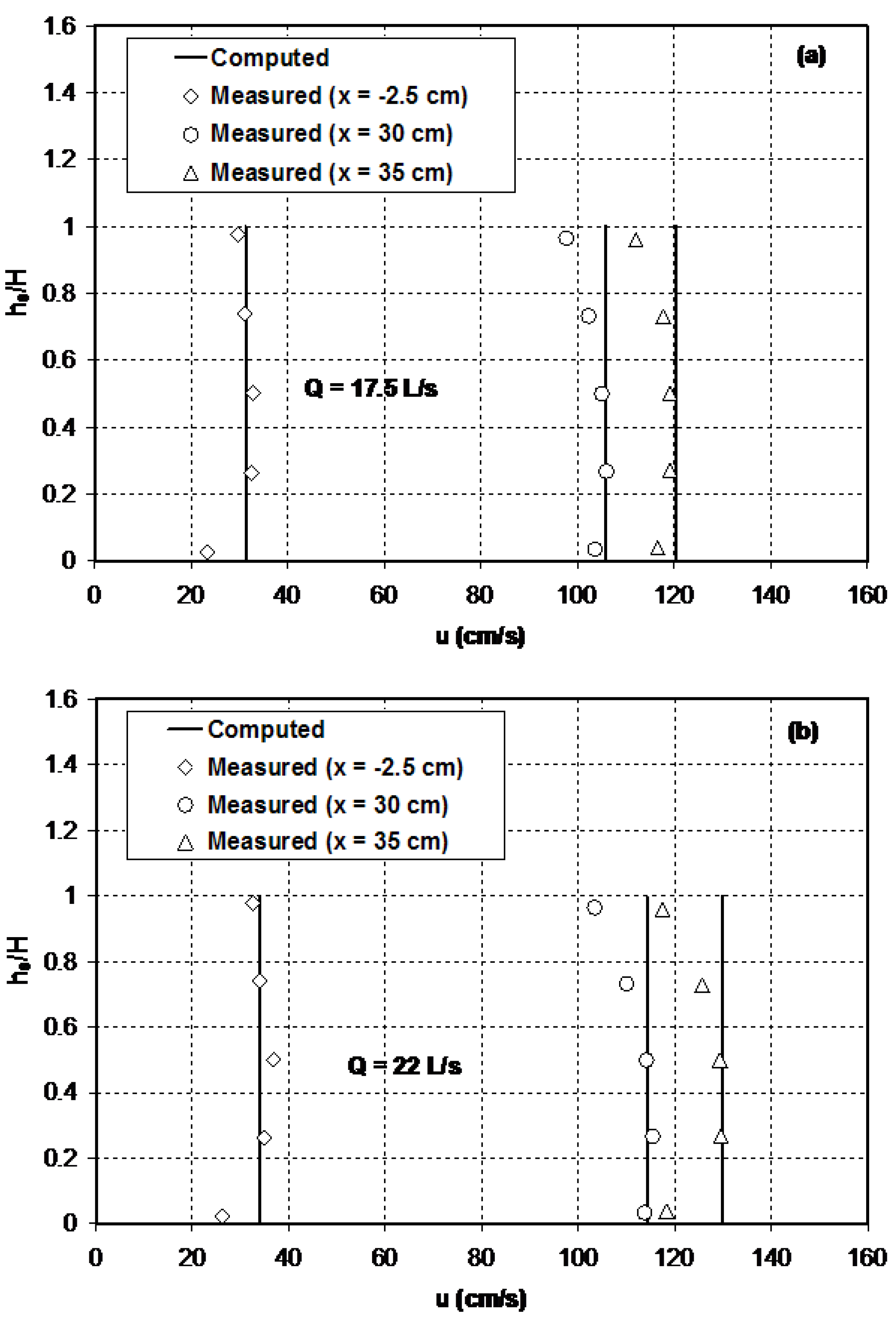
Figure 7 compares the computed horizontal velocity profiles with the laterally-averaged measured data. Although the assumed constant vertical profile for the horizontal velocity distribution is an approximation, the computed results agree fairly well with the measurements for this test case. As can be seen from
Figure 7, the flow in the narrow section of the flume attains maximum velocity at a point beneath the free surface. The values of the Boussinesq coefficient,
, were estimated for the measured velocity data using a numerical procedure developed by Zerihun [
33]. For the test case considered here, its value varies between 1.01 and 1.04.
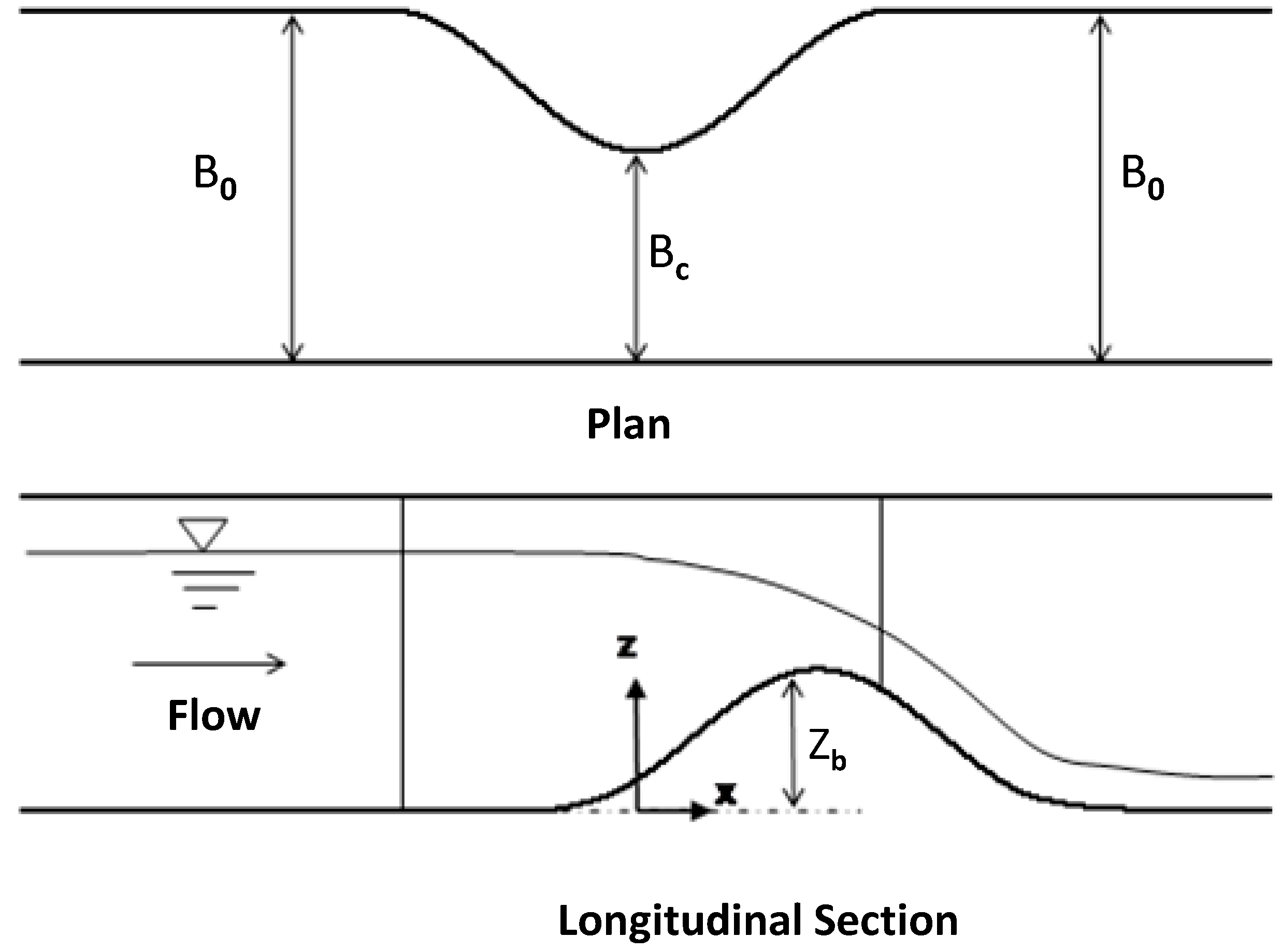
4.2. Flow in a Channel with Curved Sidewall and Bottom Hump
Measurements for free surface profiles for model validations are obtained from the experiments conducted by Law [
38]. These experiments were performed in a 16 m-long recirculating glass wall flume. At the middle of the flume, a plexiglass obstacle consisting of a sidewall protuberance and bottom hump was installed to create a channel section with a gradually-varied width and bed elevation, as shown in
Figure 8. The minimum width of the contracted section of the channel and the maximum height of bed are 94 mm and 63 mm, respectively. The shape of the profile of the hump and the width of the flume are determined by the following equations:
where
is measured horizontally in the downstream direction from the section of minimum flume width;
is the horizontal distance between the maximum contracted section and the section at the maximum height of the hump; and
= 0.06 m. A value of
= 0.20 m was adopted in order to avoid the flow separation problem in the supercritical flow region. The free surface profiles at the middle of the cross-section were measured using a point gauge with an accuracy of 0.30 mm. A detailed description of the experimental set-up and procedures can be found in Law [
38].
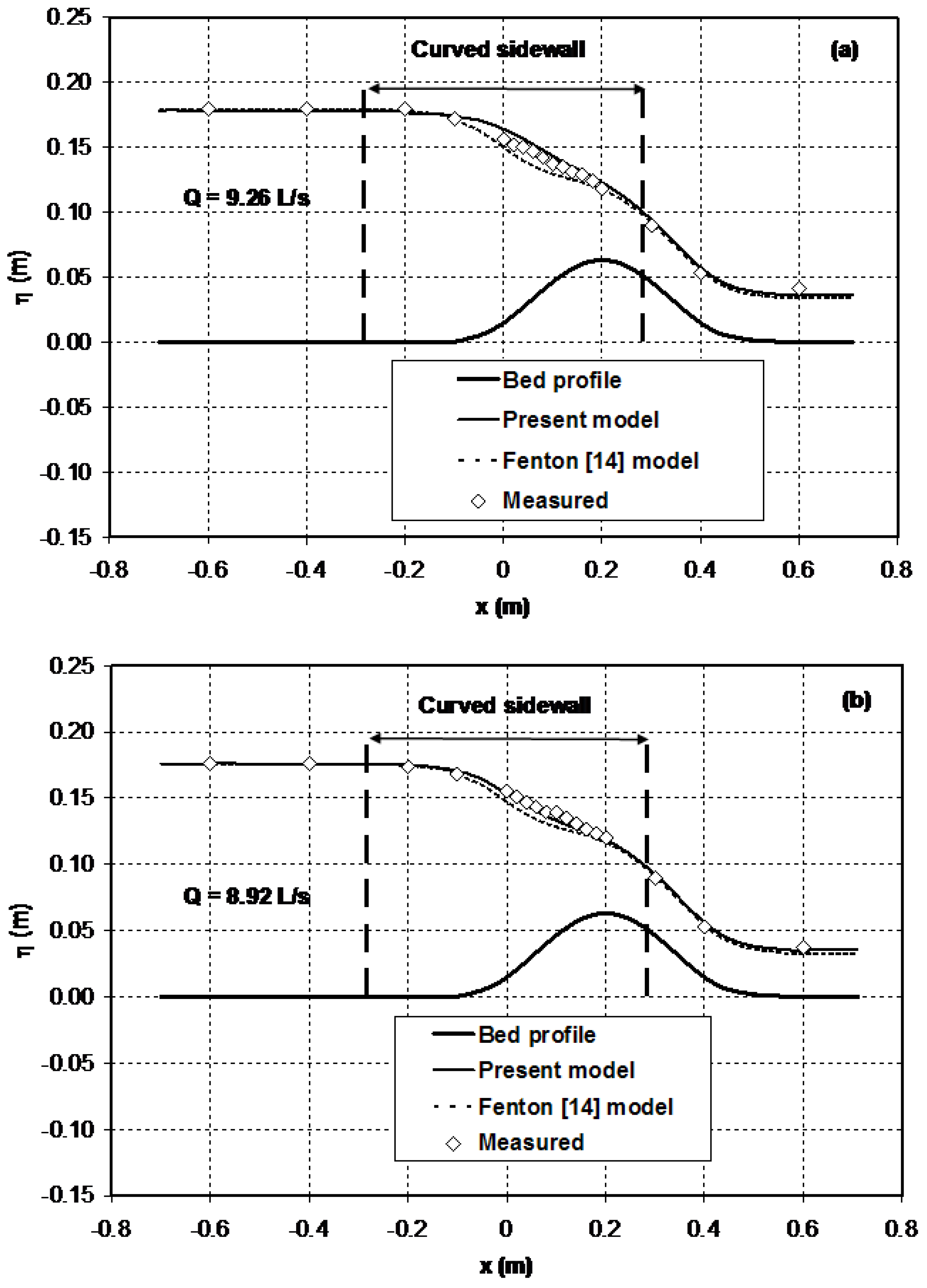
Figure 9 compares the computational results of the present model with experimental data. It also depicts the comparison of the predictions of the present model with previous results obtained by Zerihun [
33] using Fenton’s [
14] equations. In the upstream subcritical flow region, the agreement between the results of the numerical models and the experimental data is remarkable. Similar performance results can be seen in the supercritical flow region downstream of the maximum height of the hump. In general, no significant differences are observed between the numerical results of the two models in these flow regions. In the vicinity of the critical section where the combined effects of the sidewall and streamline vertical curvatures are substantial, the results of the present model compare well to the experimental data (maximum relative error = 1.6%) and are marginally better than earlier numerical results (maximum relative error = 3.5%) obtained by Zerihun [
33]. The discrepancy of Fenton’s [
14] model results from measurements in this region is attributed to the effect of sidewall curvature. For this test case, the relative bed curvature,
(
= curvature of the bed), of the flows varies from 0.29 down to −0.28. This implies that the validation scenario represents a case of transcritical flow over a moderately curved bed. Despite the flow exhibiting 3D characteristics in the vicinity of the critical section, especially at higher discharge, the performance of the present model for this test case is satisfactory.
The simulation results for flows in short-throated flumes with and without bottom humps revealed that the predictions of the present model showed improvements against the numerical results obtained by using Fenton’s [
14] and Fenton and Zerihun’s [
18] models in terms of free surface profiles and pressure distributions. The computational time of the present and previous one-dimensional non-hydrostatic models was also analysed. For all test cases, the models required almost equal simulation run-time to converge to a final steady-state solution starting from the assumed initial free surface position. A typical computational time for the problem of transcritical flow in a Venturi flume with an arc-shaped converging section was 17 s and 15 s, respectively, for the present and the Fenton and Zerihun [
18] models. These models were run on a personal computer with an Intel Core I7 processor (2.4 GHz). Ghamry and Steffler [
39] examined the computational efficiency of a quasi-3D non-hydrostatic model and the horizontal 2D shallow-water equations and found that the 3D model is computationally more expensive and requires larger memory allocation. This implies that the computational solution of the proposed model is more robust than that of a quasi-3D model. In engineering practice, this model serves as a numerical tool for designing the height of the sidewalls of a chute spillway and developing or modifying a concept design to minimise excessive negative pressure over the crest of an overflow structure.
The capability of the model for developing head-discharge relationships for critical-flow flumes under free flow conditions will be examined in the next section. It is important to note that this investigation is limited to free flows in horizontal bed rectangular Venturi flumes.
6. Discussion
As described before, the geometric features of the Venturi flume are designed to minimise the total energy loss when it is operated under the modular flow condition. The total energy loss is estimated by considering the effects of the roughness of the flume and the turbulence of the flow. Experimental evidence shows that a large percentage of the total energy loss is due to friction. The turbulence characteristics of the flow, which depend on the contraction and expansion ratios of the flume, the Froude number and Reynolds number [
44], strongly determine the strength of the energy dissipating turbulent eddies. In the contraction section of the flume, the flow possesses high convective acceleration, which distorts the velocity and shear stress distributions and leads to excessive turbulence and flow separation from the sidewalls. Furthermore, the incoming flow Froude number gradually increases and approaches unity near the critical section. Consequently, the horizontal and vertical turbulence intensities increase in the streamwise direction near the free surface and walls [
44]. By properly designing the geometric shape of the inlet contraction section, one can avoid the flow separation problem and maximise the hydraulic performance of the critical-flow flume (see, e.g., [
45]).
On the other hand, in the diverging section of the flume, the flow decelerates due to increasing flow cross-sectional area. Under a steady flow condition, flow deceleration triggers flow separation and turbulent eddies, which results in the dissipation of kinetic energy. Part of the remaining kinetic energy of the flow is transformed into potential energy and is conserved as an elevation head. Similar to the contraction section, the Froude and Reynolds numbers slightly influence the turbulence intensities of the flow. The result of an experimental study reveals that the flow patterns in a perfect symmetrical sudden diverging section are asymmetrical [
46], which makes the geometric feature undesirable in practice. Although the method is relatively expensive, gradual expansion of the diverging section can avoid flow separation and increases the hydraulic efficiency of the critical-flow flume. The total energy loss in open channel flow-measuring structures can be deduced from the momentum and energy principles (see, e.g., [
3,
47]). Nonetheless, the energy method utilises the pre-assumed energy loss coefficients, which are very likely to be subject to errors. A higher-order numerical model that allows for turbulence friction is an alternative approach for predicting the 3D structure of the flow, thereby quantifying the total energy losses. The 2D non-hydrostatic version of the current model for turbulent open channel flows is under development.
7. Conclusions
A novel approach, which employs the Serre [
27] approximation, has been applied to develop a one-dimensional non-hydrostatic model for open channel flows in short-throated flumes. The developed model incorporates a higher-order dynamic pressure correction for the effects of the sidewalls and streamline vertical curvatures. The improvement of the proposed model over previous works is its capacity to model the local flow characteristics of strongly-curved flows in Venturi flumes with rounded or broken plane transition. The model equations were discretised using the finite difference approximations, which resulted in a system of nonlinear algebraic equations. These nonlinear algebraic equations were solved iteratively using the Newton–Raphson method with the numerically-determined Jacobian matrix. The model was then applied to simulate the important aspects of curvilinear flows in short-throated flumes with a contraction ratio between 0.38 and 0.62. A comparison of the model results with the corresponding experimental data and earlier numerical results was also presented.
For free flow in a Parshall flume, the proposed model satisfactorily predicted the free surface profile, which agreed well with the 2D model result. Compared to Fenton and Zerihun’s [
18] model, the present model accurately described the pressure distributions for flows in a horizontal bed short-throated flume with rounded transition. For curvilinear flows in a channel with a curved sidewall and bottom hump, the results of the present model compared well to the experimental data and were marginally better than earlier numerical results obtained by Zerihun [
33], especially in the vicinity of the critical section where the combined effects of the sidewall and streamline vertical curvatures are substantial. Generally speaking, the overall performance of the present model for curvilinear flows in short-throated flumes was reasonably good.
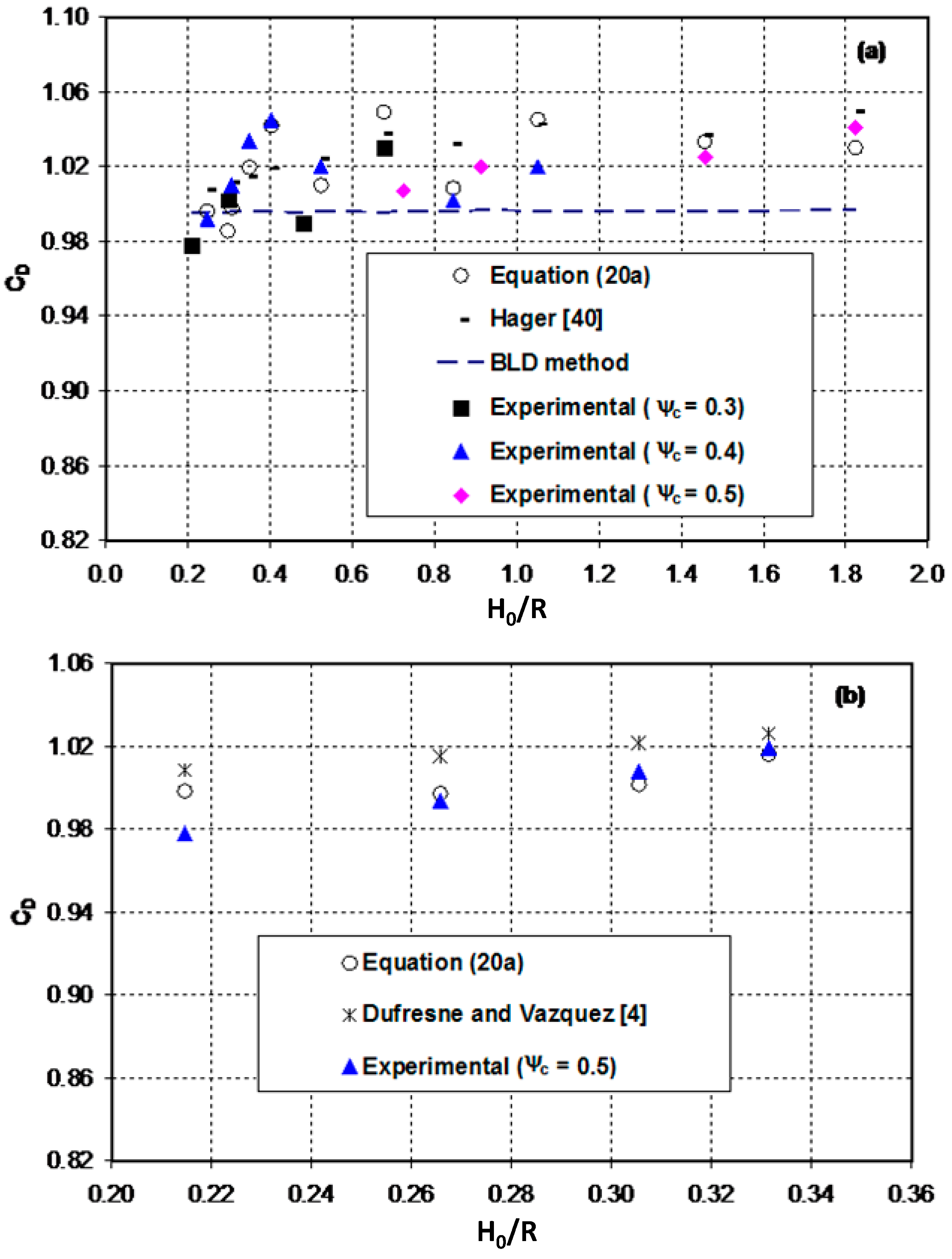
A universal method, which is valid for long, intermediate and short throat-length flumes, has been proposed for computing the discharge coefficients. The comparison of the computed results with measurements highlights the power and potential of the proposed method for developing discharge rating curves for critical-flow flumes under free flow conditions. With the demonstrated satisfactory performance, the proposed model has the potential to be used as a numerical tool for developing design guidelines and assessing the hydraulic performance of flow-measuring structures.


