
Modeling the Viscoelastic Behavior of Amorphous Shape Memory Polymers at an Elevated Temperature

Abstract
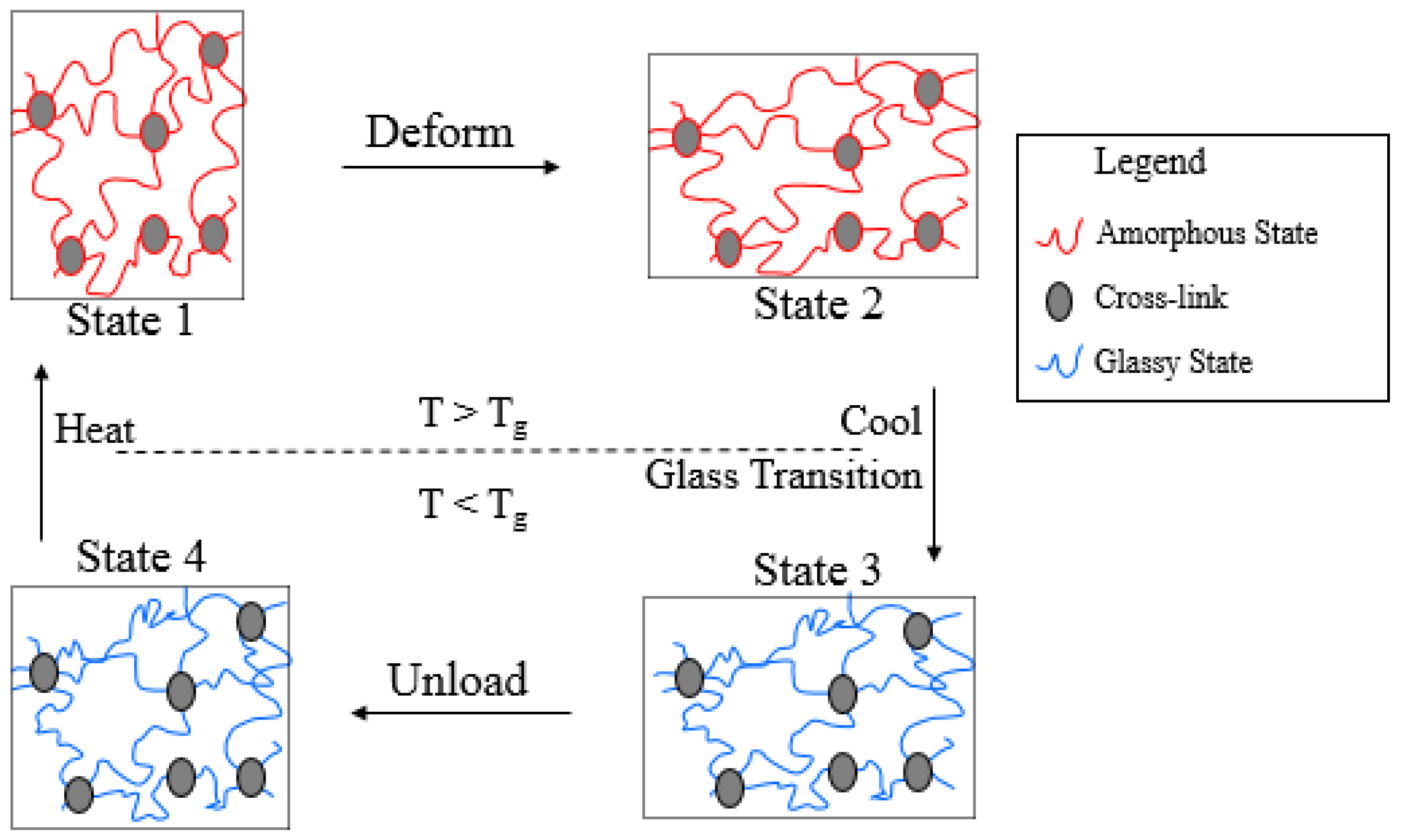
:1. Introduction
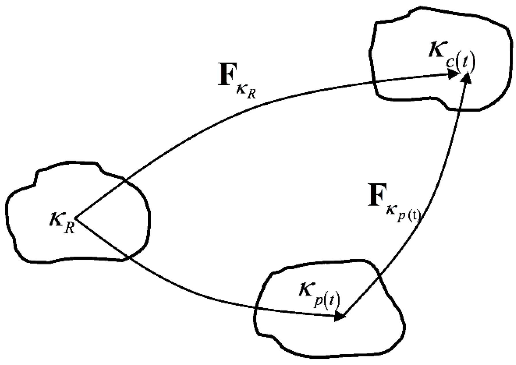
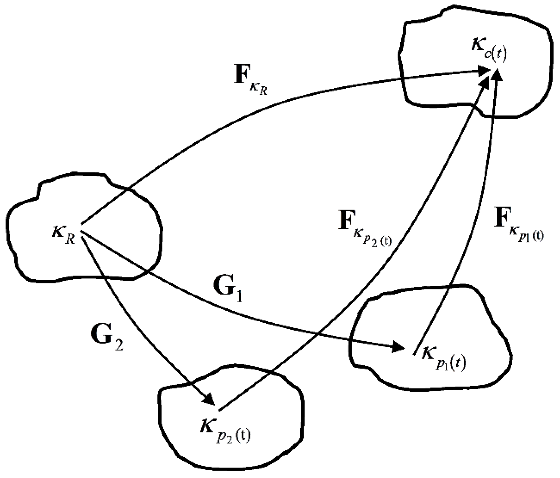
2. Preliminaries
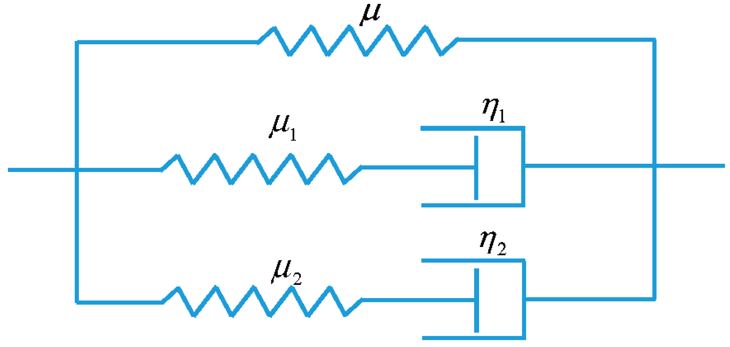
3. Model Description
3.1. Hyperelsatic Behavior of the Equilibrium Branch
3.2. Viscoelastic Behavior of the Non-Equilibrium Branch
3.3. Model Conclusion
4. Applications
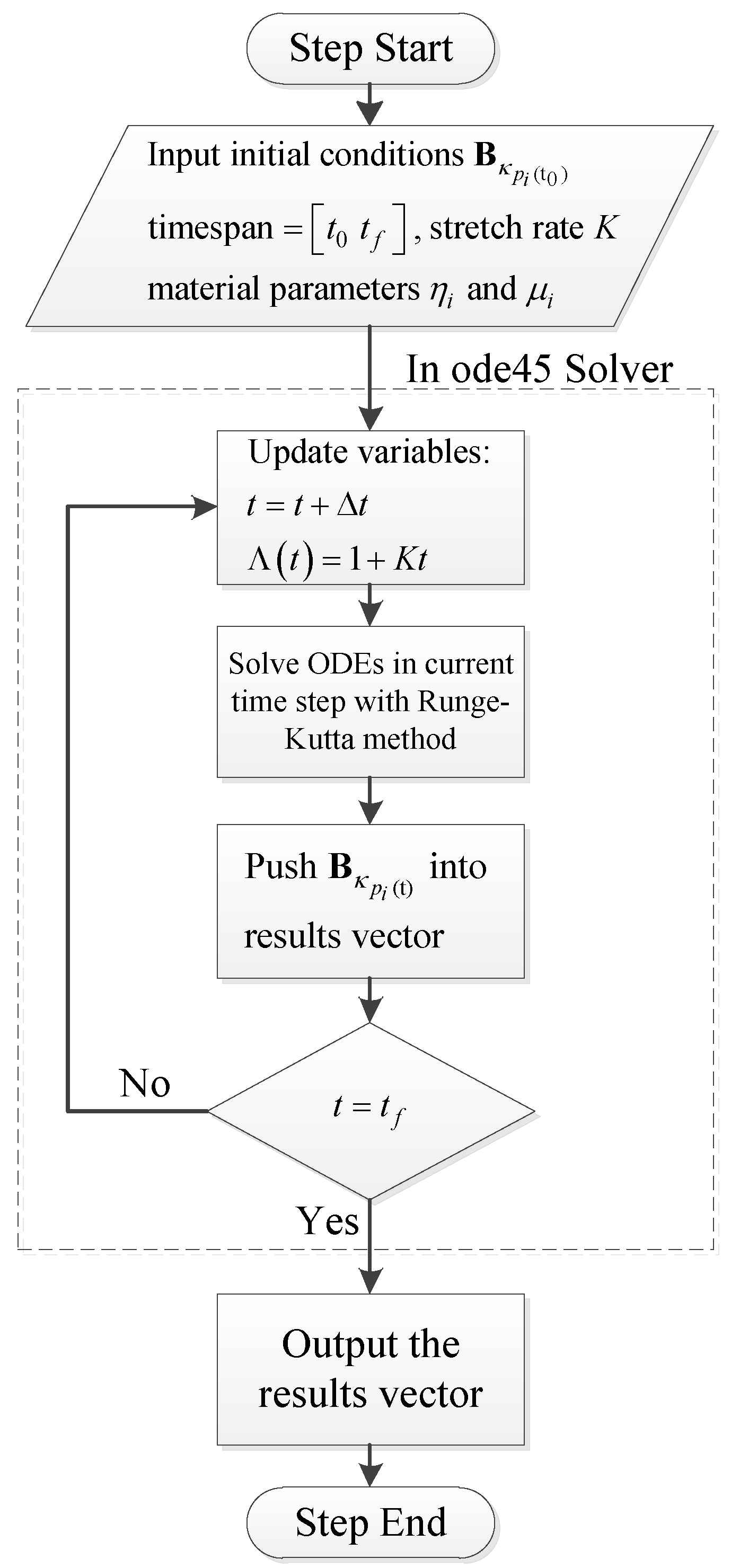
4.1. Numerical Procedure
4.2. Parameter Identification
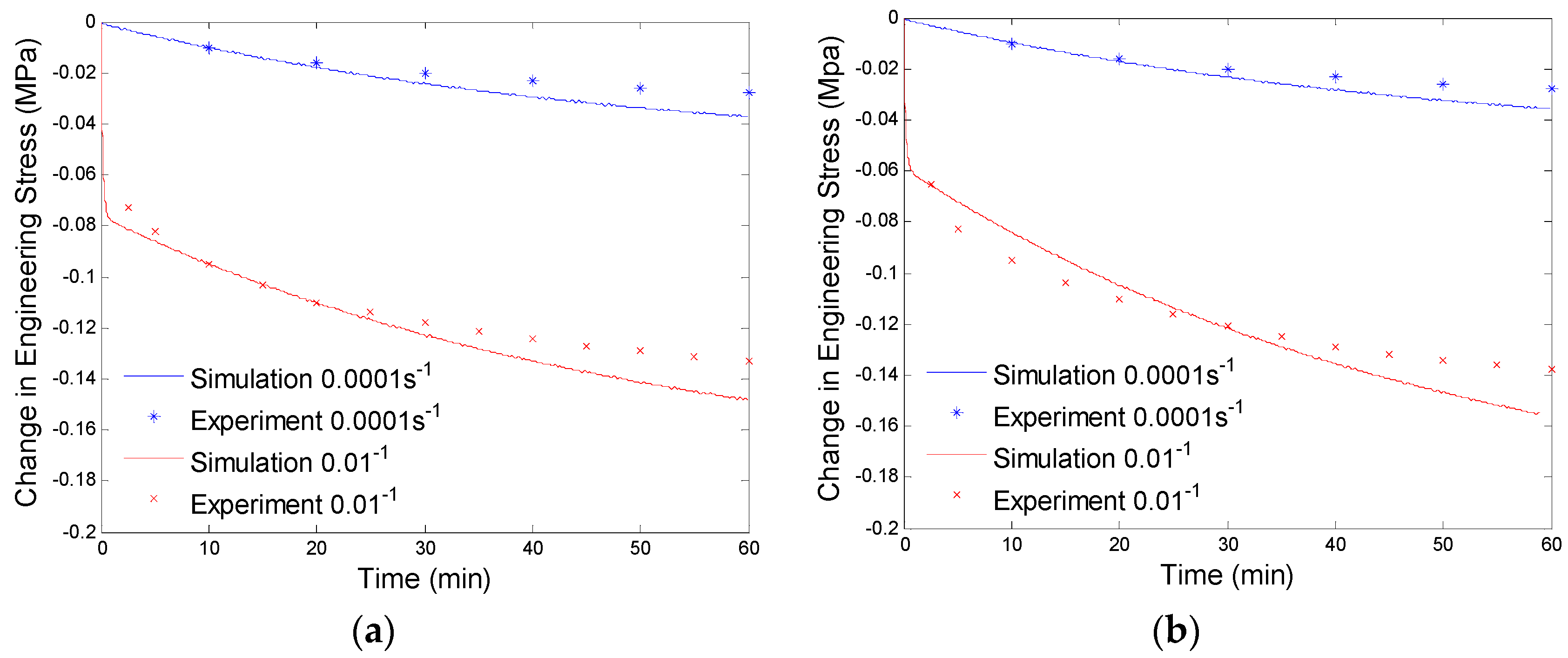
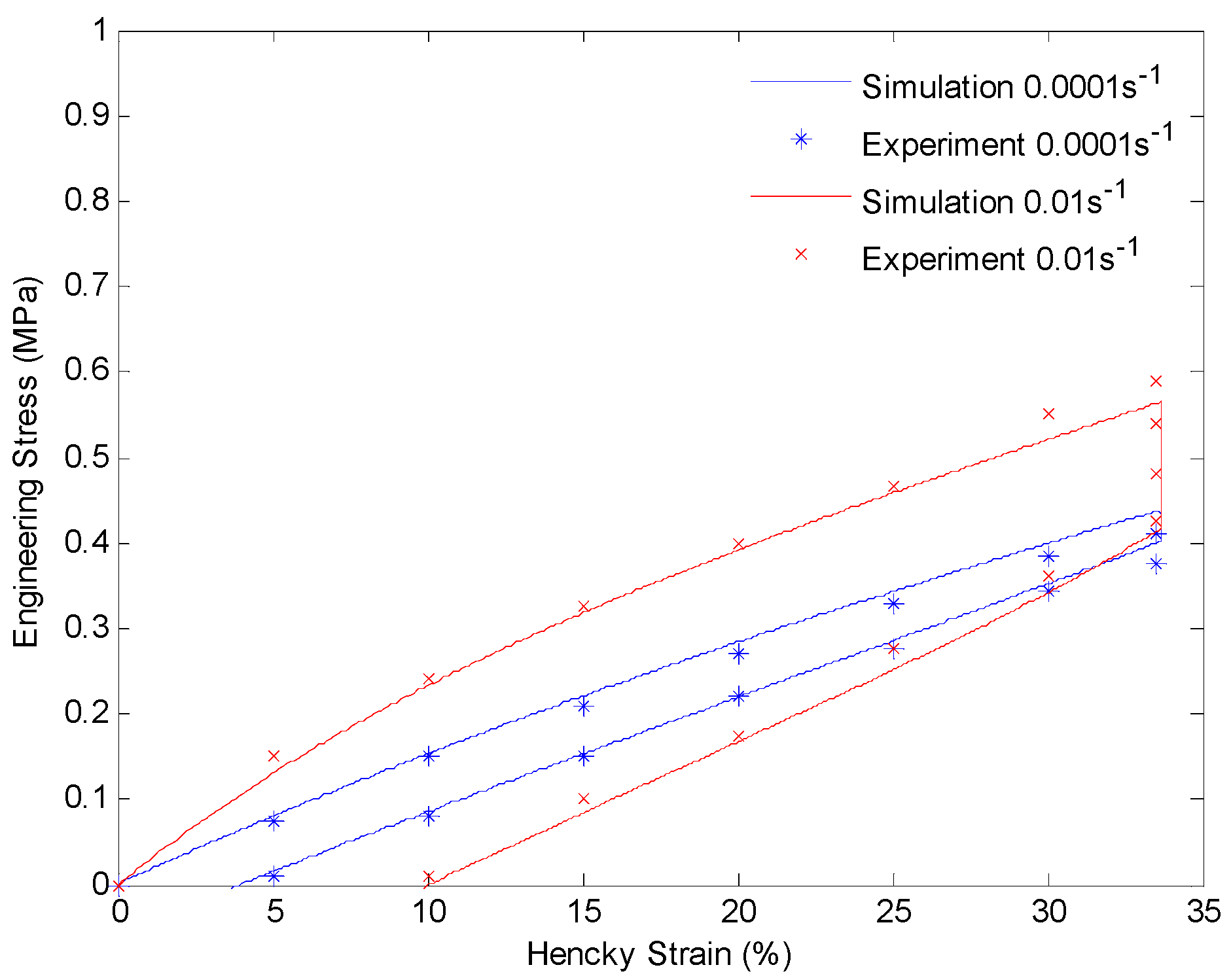
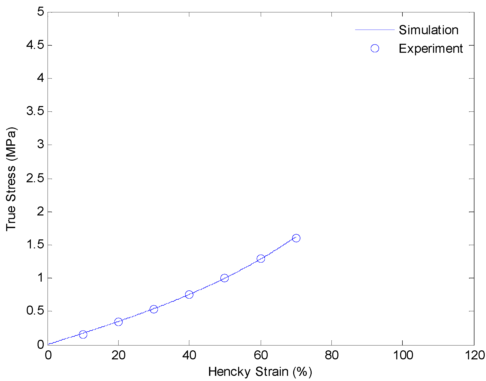
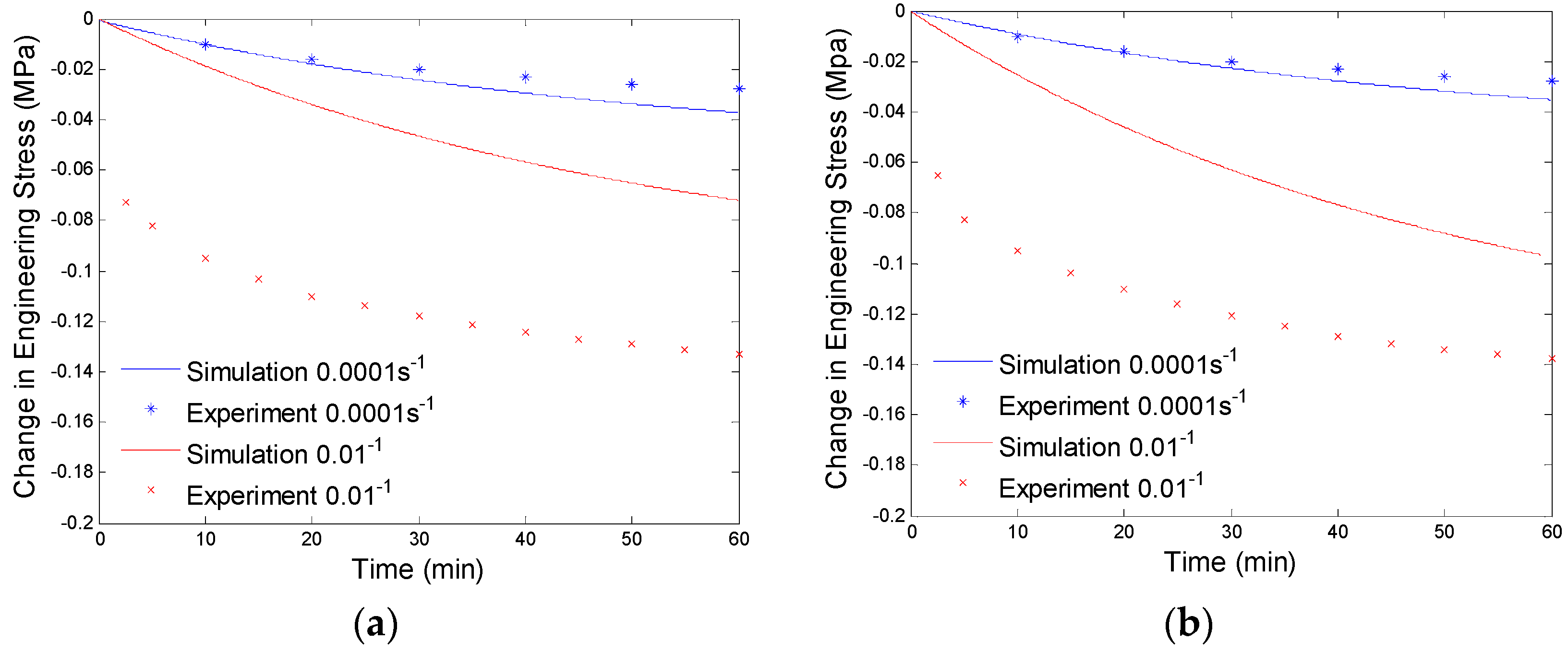
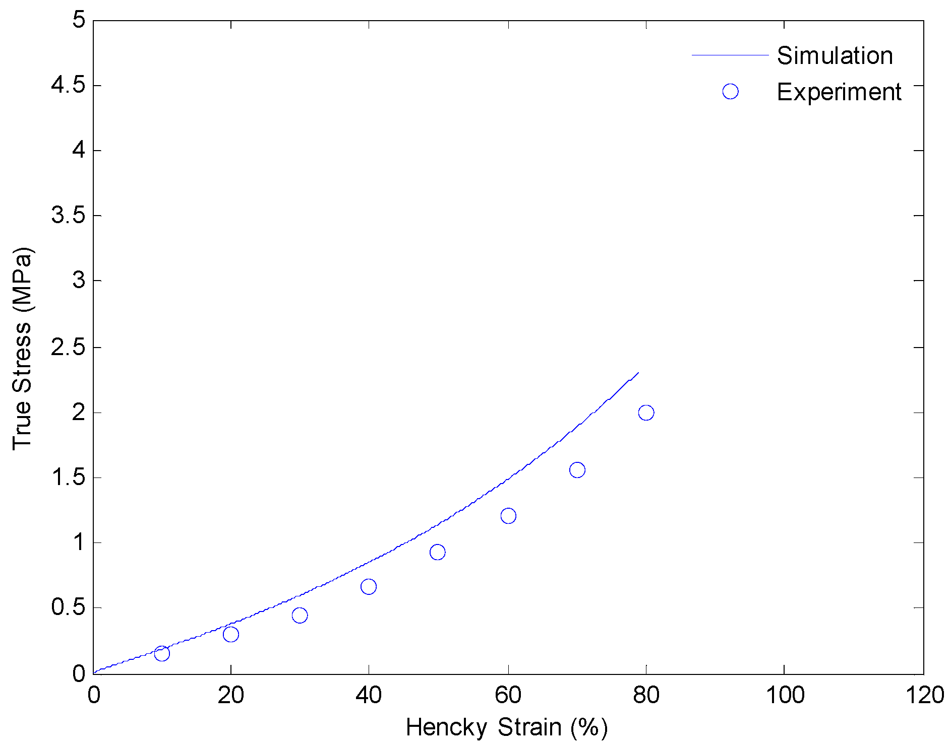
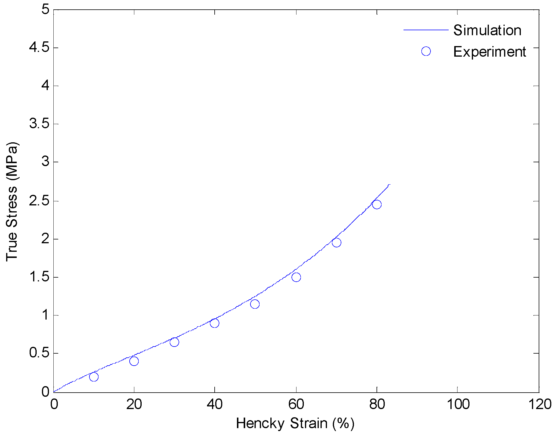
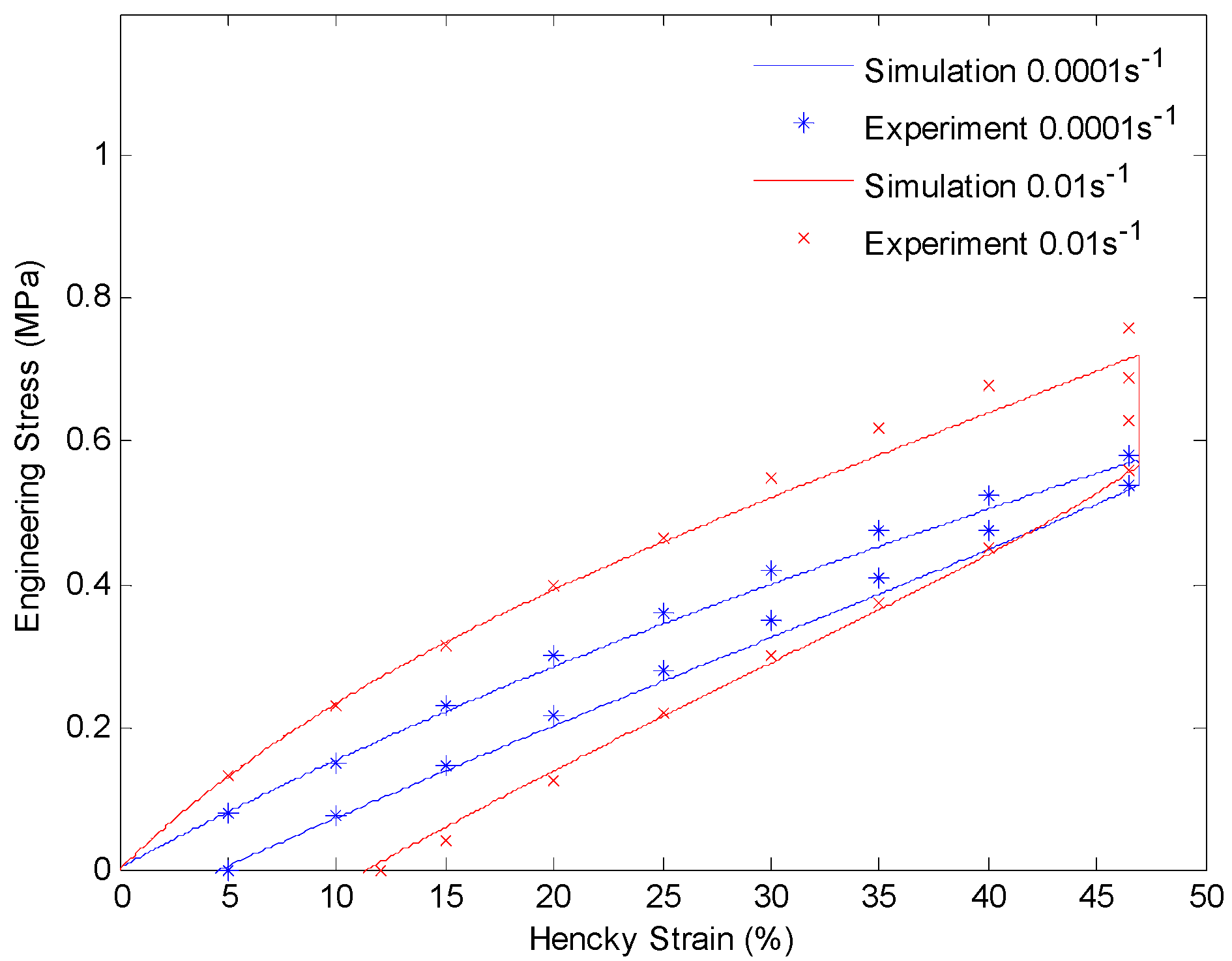
4.3. Results and Discussion
5. Conclusions
Acknowledgments
Author Contributions
Conflicts of Interest
References
- Lendlein, A.; Kelch, S. Shape-memory polymers. Angew. Chem. Int. Ed. 2002, 41, 2035–2057. [Google Scholar] [CrossRef]
- Lendlein, A.; Schmidt, A.M.; Langer, R. AB-polymer networks based on oligo(ε-caprolactone) segments showing shape-menory properties. Proc. Natl. Acad. Sci. USA 2001, 98, 842–847. [Google Scholar] [PubMed]
- Ge, Q.; Luo, X.; Iversen, C.B.; Mather, P.T.; Dunn, M.L.; Qi, H.J. Mechanisms of triple-shape polymeric composites due to dual thermal transitions. Soft Matter 2013, 9, 2212–2223. [Google Scholar] [CrossRef]
- Lendlein, A.; Jiang, H.; Jünger, O.; Langer, R. Light-induced shape-memory polymers. Nature 2005, 434, 879–882. [Google Scholar] [CrossRef] [PubMed]
- Wu, L.; Jin, C.; Sun, X. Synthesis, properties, and light-induced shape memory effect of multiblock polyesterurethanes containing biodegradable segments and pendant cinnamamide groups. Biomacromolecules 2011, 12, 235–241. [Google Scholar] [CrossRef] [PubMed]
- Lu, H.B.; Huang, W.M.; Yao, Y.T. Review of chemo-responsive shape change/memory polymers. Pigment Resin Technol. 2013, 42, 237–246. [Google Scholar] [CrossRef]
- Schmidt, A.M. Electromagnetic activation of shape memory polymer networks containing magnetic nanoparticles. Macromol. Rapid Commun. 2006, 27, 1168–1172. [Google Scholar] [CrossRef]
- Buckley, P.R.; McKinley, G.H.; Wilson, T.S.; Small, W.; Benett, W.J.; Bearinger, J.P.; McElfresh, M.W.; Maitland, D.J. Inductively heated shape memory polymer for the magnetic actuation of medical devices. IEEE Trans. Biomed. Eng. 2006, 53, 2075–2083. [Google Scholar] [CrossRef] [PubMed]
- Du, H.; Zhang, J. Solvent induced shape recovery of shape memory polymer based on chemically cross-linked poly(vinyl alcohol). Soft Matter 2010, 6, 3370–3376. [Google Scholar] [CrossRef]
- Liu, C.; Qin, H.; Mather, P.T. Review of progress in shape-memory polymers. J. Mater. Chem. 2007, 17, 1543–1558. [Google Scholar] [CrossRef]
- Xue, L.; Dai, S.; Li, Z. Biodegradable shape-memory block co-polymers for fast self-expandable stents. Biomaterials 2010, 31, 8132–8140. [Google Scholar] [CrossRef] [PubMed]
- Wei, Z.G.; Sandström, R.; Miyazaki, S. Shape-memory materials and hybrid composites for smart systems—Part I Shape-memory materials. J. Mater. Sci. 1998, 33, 3743–3762. [Google Scholar] [CrossRef]
- Yakacki, C.M.; Shandas, R.; Lanning, C.; Rech, B.; Eckstein, A.; Gall, K. Unconstrained recovery characterization of shape-memory polymer networks for cardiovascular applications. Biomaterials 2007, 28, 2255–2263. [Google Scholar] [CrossRef] [PubMed]
- Eisenhaure, J.D.; Rhee, S.I.; Al-Okaily, A.M.; Carlson, A.; Ferreira, P.M.; Kim, S. The use of shape memory polymers for MEMS assembly. J. Microelectromech. Syst. 2015, 25, 69–77. [Google Scholar] [CrossRef]
- Gall, K.; Kreiner, P.; Turner, D.; Hulse, M. Shape-memory polymers for microelectromechanical systems. J. Microelectromech. Syst. 2004, 13, 472–483. [Google Scholar] [CrossRef]
- Ge, Q.; Dunn, C.K.; Qi, H.J.; Dunn, M.L. Active origami by 4D printing. Smart Mater. Struct. 2014, 23, 094007. [Google Scholar] [CrossRef]
- Yu, K.; Dunn, M.L.; Qi, H.J. Digital manufacture of shape changing components. Extreme Mech. Lett. 2015, 4, 9–17. [Google Scholar] [CrossRef]
- Liu, Y.; Gall, K.; Dunn, M.L.; Greenberg, A.R.; Diani, J. Thermomechanics of shape memory polymers: Uniaxial experiments and constitutive modeling. Int. J. Plast. 2006, 22, 279–313. [Google Scholar] [CrossRef]
- McClung, A.J.W.; Tandon, G.P.; Baur, J.W. Strain rate- and temperature-dependent tensile properties of an epoxy-based, thermosetting, shape memory polymer (Veriflex-E). Mech. Time Depend. Mater. 2012, 16, 205–221. [Google Scholar] [CrossRef]
- McClung, A.J.W.; Tandon, G.P.; Baur, J.W. Deformation rate-, hold time-, and cycle-dependent shape-memory performance of Veriflex-E resin. Mech. Time Depend. Mater. 2013, 17, 39–52. [Google Scholar] [CrossRef]
- Rajagopal, K.R.; Srinivasa, A.R. On the inelastic behavior of solids—Part 1: Twinning. Int. J. Plast. 1995, 11, 653–678. [Google Scholar] [CrossRef]
- Rajagopal, K.R.; Wineman, A.S. A constitutive equation for nonlinear solids which undergo deformation induced microstructural changes. Int. J. Plast. 1992, 8, 385–395. [Google Scholar] [CrossRef]
- Rajagopal, K.R.; Srinivasa, A.R. On the thermomechanics of shape memory wires. Z. Angew. Math. Phys. 1999, 50, 459–496. [Google Scholar]
- Rajagopal, K.R.; Srinivasa, A.R. A thermodynamic frame work for rate type fluid models. J. Non-Newton. Fluid Mech. 2000, 88, 207–227. [Google Scholar] [CrossRef]
- Karra, S.; Rajagopal, K.R. A thermodynamic framework to develop rate-type models for fluids without instantaneous elasticity. Acta Mech. 2009, 205, 105–119. [Google Scholar] [CrossRef]
- Rao, I.J.; Rajagopal, K.R. Study of strain-induced crystallization of polymers. Int. J. Solids Struct. 2001, 38, 1149–1167. [Google Scholar] [CrossRef]
- Rao, I.J.; Rajagopal, K.R. On the modeling of quiescent crystallization of polymer melts. Polym. Eng. Sci. 2004, 44, 123–130. [Google Scholar] [CrossRef]
- Rao, I.J.; Rajagopal, K.R. A thermodynamic framework for the study of crystallization in polymers. Z. Angew. Math. Phys. 2002, 53, 365–406. [Google Scholar] [CrossRef]
- Moon, S.; Cui, F.; Rao, I.J. Constitutive modeling of the mechanics associated with triple shape memory polymers. Int. J. Eng. Sci. 2015, 96, 86–110. [Google Scholar] [CrossRef]
- Barot, G.; Rao, I.J. Constitutive modeling of the mechanics associated with crystallizable shape memory polymers. Z. Angew. Math. Phys. 2006, 57, 652–681. [Google Scholar] [CrossRef]
- Barot, G.; Rao, I.J.; Rajagopal, K.R. A thermodynamic framework for the modeling of crystallizable shape memory polymers. Int. J. Eng. Sci. 2008, 46, 325–351. [Google Scholar] [CrossRef]
- Sodhi, J.S.; Rao, I.J. Modeling the mechanics of light activated shape memory polymers. Int. J. Eng. Sci. 2010, 48, 1576–1589. [Google Scholar] [CrossRef]
- Sodhi, J.S.; Cruz, P.R.; Rao, I.J. Inhomogeneous deformations of light activated shape memory polymers. Int. J. Eng. Sci. 2015, 89, 1–17. [Google Scholar] [CrossRef]
- Westbrook, K.K.; Kao, P.H.; Castro, F.; Ding, Y.; Jerry, Q.H. A 3D finite deformation constitutive model for amorphous shape memory polymers: A multi-branch modeling approach for nonequilibrium relaxation processes. Mech. Mater. 2011, 43, 853–869. [Google Scholar] [CrossRef]
- O’Connell, P.A.; McKenna, G.B. Arrhenius-type temperature dependence of the segmental relaxation below Tg. J. Chem. Phys. 1999, 110, 11054–11060. [Google Scholar] [CrossRef]
- Williams, M.L.; Landel, R.F.; Ferry, J.D. The temperature dependence of relaxation mechanisms in amorphous polymers and other glass-forming liquids. J. Am. Chem. Soc. 1955, 77, 3701–3707. [Google Scholar] [CrossRef]


| Description | Parameters | Values |
|---|---|---|
| Equilibrium Branch Parameter | ||
| Shear Modulus (MPa) | μ | 0.43 × 10⁶ |
| Non-equilibrium Branch Parameters | ||
| Shear Modulus of Branch One (MPa) | μ1 | 0.117 × 10⁶ |
| Viscosity of Branch One (MPa·s) | η1 | 350 × 106 |
| Shear Modulus of Branch Two (MPa) | μ2 | 0.43 × 10⁶ |
| Viscosity of Branch Two (MPa·s) | η2 | 4.3 × 10⁶ |
© 2016 by the authors; licensee MDPI, Basel, Switzerland. This article is an open access article distributed under the terms and conditions of the Creative Commons Attribution license ( http://creativecommons.org/licenses/by/4.0/).
Share and Cite
Cui, F.; Moon, S.; Rao, I.J. Modeling the Viscoelastic Behavior of Amorphous Shape Memory Polymers at an Elevated Temperature. Fluids 2016, 1, 15. https://doi.org/10.3390/fluids1020015
Cui F, Moon S, Rao IJ. Modeling the Viscoelastic Behavior of Amorphous Shape Memory Polymers at an Elevated Temperature. Fluids. 2016; 1(2):15. https://doi.org/10.3390/fluids1020015
Chicago/Turabian StyleCui, Fangda, Swapnil Moon, and I. Joga Rao. 2016. "Modeling the Viscoelastic Behavior of Amorphous Shape Memory Polymers at an Elevated Temperature" Fluids 1, no. 2: 15. https://doi.org/10.3390/fluids1020015