
Splash Dynamics of Paint on Dry, Wet, and Cooled Surfaces


Complex Fluids Lab, Montclair State University, 1, Normal Avenue, Montclair, NJ 07043, USA
*
Author to whom correspondence should be addressed.
Fluids 2016, 1(2), 12; https://doi.org/10.3390/fluids1020012
Submission received: 22 December 2015
/
Revised: 21 March 2016
/
Accepted: 8 April 2016
/
Published: 14 April 2016
(This article belongs to the Special Issue Rheology and the Thermo-Mechanics of Non-Newtonian Fluids)
Abstract
:In his classic study in 1908, A.M. Worthington gave a thorough account of splashes and their formation through visualization experiments. In more recent times, there has been renewed interest in this subject, and much of the underlying physics behind Worthington’s experiments has now been clarified. One specific set of such recent studies, which motivates this paper, concerns the fluid dynamics behind Jackson Pollock’s drip paintings. The physical processes and the mathematical structures hidden in his works have received serious attention and made the scientific pursuit of art a compelling area of exploration. Our current work explores the interaction of watercolors with watercolor paper. Specifically, we conduct experiments to analyze the settling patterns of droplets of watercolor paint on wet and frozen paper. Variations in paint viscosity, paper roughness, paper temperature, and the height of a released droplet are examined from time of impact, through its transient stages, until its final, dry state. Observable phenomena such as paint splashing, spreading, fingering, branching, rheological deposition, and fractal patterns are studied in detail and classified in terms of the control parameters.
1. Introduction
The relationship between fluid mechanics and art is a certainly not a new field of investigation within mathematics and physics. Leonardo da Vinci’s pioneering studies and detailed sketches of water flow date back to 1508. The series of block prints of great waves by Japanese artist Hokusai were published around 1830 [1]. More recently, fractal patterns and dimension have become fascinating and fertile areas of scientific interest, most notably with the use of viscous oils, latex paints, and varnish fixatives. Recent studies of Jackson Pollock’s drip paintings are widely known and quite compelling, as are the analyses of varnish crackling, used to authenticate paintings by the great masters [2,3]. However, the physics and mathematics of watercolor painting remains largely unexplored. This could, in large part, be due to the fact that water quickly disperses, along with the pigment. Furthermore, watercolors permeate the underlying sheet of paper rather than drying on top of a canvas, a phenomenon observed with the more viscous media. This experiment explores droplet patterns of watercolors with the aim of elucidating the physics behind the process. The results thus far have been quite interesting and varied with respect to the kinds of fractals produced, branches and tributaries, rheological formations, and residual sediment patterns to name a few. Watercolor appears to be a great medium to explore the art of fluid dynamics, or perhaps the fluid dynamics of art, due to water’s complex behavior, ultimately yielding some truly spectacular displays.
The dynamics of a splash, such as one produced by the impact of a droplet on a surface has been extremely well studied and the literature on the subject dates back to 1908 to the work by Worthington [4,5]. The subject continues to be of interest in current times as well due to diverse applications such as in forensics, ink-jet printing and micro-fabrication processes which rely upon drop dispensing. Recent review papers [6,7,8] discuss the state of the art in the field up until the last decade. In this regard, the studies concerning the impact of droplets on dry surfaces is most relevant to our own work. The experimental work by Rioboo et al. [9] explored the impact of different liquids upon solid surfaces corresponding to varying surface roughness. Their investigations revealed six categories of splashes: deposition, prompt splash, coronal splash, receding break-up, partial rebound and complete rebound, which depend upon the properties of the liquid and surface. In addition to the roughness of the surface, the viscosity, density and surface tension of the liquid droplet have been recognized as being significant and the different regimes of droplet splashes are often expressed in terms of three dimensionless quantities, namely the Reynolds (), Weber () and Ohnesorge () numbers [8] which depend upon these afore-mentioned physical parameters. The viscosity of the droplet and friction of the surface determines the initial stages of the splash while the surface tension takes control of the final stages, when the drop thickness on the surface is diminished. The prominent regimes are distinguished by the parameter whose critical value determines the onset of splashing.
There has also been a substantial amount of work on the splash patterns of non-Newtonian and particle-laden droplets (see for instance [10,11,12,13,14]). As is expected, non-Newtonian characteristics such as viscoelasticity, yield-stress and shear-thinning result in a marked variation in the observed post-impact behavior of the droplets. These have been categorized as (a) irreversible viscoplastic behavior, (b) perfect elastic recoil and (c) viscoleasticity [11]. In the case of non-Newtonian fluids, the Deborah number (), critical strain parameter () and Mach number (M) have been used to classify the various observed regimes. The splash dynamics of droplets with embedded particles is equally interesting and unique [13,14,15]. For droplets with a sufficiently low particle concentration, the parameter K has been employed to characterize the drop impact with the viscosity μ replaced by an effective, concentration-dependent viscosity . In the case of high concentration droplets, it is observed that a reinterpretation of the Weber number, based on particle characteristics, is needed to accurately capture the onset of splashing.
The present article presents our experimental results for droplets of watercolor impacting wetted canvas, which are maintained at different temperatures at and below room temperature. Our observations are contrasted with those reported in the literature and inform an unexplored aspect of the bigger problem, which could be of interest to scientists and artists alike. The outline of the paper is as follows. In Section 2, we discuss the experimental setup and procedure. Section 3 presents the results of the experiments such as radial growth curves of the droplet patterns and effect of the control parameters upon the drop shape and size. Section 4 is focused on the fractal characteristics of the splash patterns. Finally, in Section 5, we perform a rigorous statistical study of the experiments to firmly establish causal relationships for the observed patterns.
2. Experimental Section
Materials and Methods
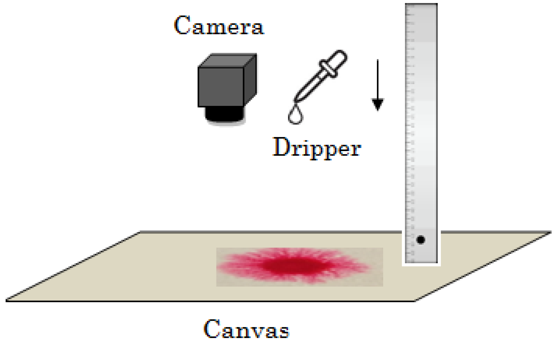
This experiment was conducted utilizing three types of Winsor and Newton Artist Series watercolor paint, namely, Permanent Rose, Prussian Blue, and Sepia. These pigments were chosen based upon their individual and significantly differing rheological, deposition properties. Each color was available in tube form whereby the pigment was squeezed from the tube and dissolved in clean, filtered water. Three grades of acid-free watercolor paper were used: Arches 140 lb rough, Arches 140 LB cold-press, and Canson 90 lb paper. The papers were cut into smaller pieces measuring roughly 5 in × 7 in and liquid frisket was applied to the edges of each rectangular paper to create a thin latex border in order to reduce and contain water dispersion. Filtered water was then applied with a soft sea sponge to both sides of the paper, a technique known as wet-on-wet, and the paper (or substrate) was mounted flat on a backing board. Excess water was spilled off, and the paper was left to sit for a few minutes to allow the substrate to thoroughly absorb water. The papers were then separated into three categories: unfrozen, frozen for 5 min, or frozen for 30 min A droplet of paint was released onto a substrate from a height of either 6 inches or 12 inches. For the first set of paintings, the droplet was released from a standard drinking straw by holding the thumb over the top, open end, removing the thumb and letting gravity pull down the pigment. For the remaining sets of paintings, a medicine dropper (of outer diameter 4 mm and inner nozzle diameter 1mm) was used to release the droplets. Photographs were taken with a cellular phone camera at roughly 1 min intervals for about 20 min or until the paint spread reached a maximum dispersion. Each digital photograph was analyzed using the ImageJ software (National Institute of Health, Bethesda, MD, USA.)
The volume of each droplet released from the medicine dropper was, on average, about 0.04 mL, while the volume released from the straw was about 0.18 mL. The density, ρ, of the droplets of the different paints was measured by weighing 10 mL of the solutions and the volume of each droplet was measured by counting the number of drops that made up 10 mL. The density of the different paints ranged between 0.99–1.02 gm/cc. The viscosity of the paints, μ, was measured using a hand held viscometer and is described in further detail later in this section. The surface tension of the watercolor paints, σ, could not be measured and was therefore assumed to be the same as that of water. The impact velocity of the droplet from the two different heights was computed using the elementary kinematic formula, , where refers to the terminal, impact velocity of the droplet, released from a height h. We find that and . Using these parameters, we can estimate the values of the non-dimensional Weber number and Reynolds number which are given by
where D refers to the characteristic length in the problem which was taken to be the approximate diameter of the droplet. In this study, the Weber number ranged between 150–323, while the Reynolds number varied from 2600–10,200. Comparing with the vs. curve shown in ([17], Figure 1), we note that our experimental conditions put us in a very interesting part of the phase map which is between the viscous-inertial and capillary-inertial spreading regimes.
Rheology of paint: The rheological properties of the materials used for painting are each important in their respective ways and interact differently with the other agents involved in the process of painting [16]. Overall, we need to pay particular attention to the following: (1) the support in these experiments: namely the watercolor paper; (2) the ground: the first layer on the support, i.e., the water applied to the paper; (3) the paint: one or more pigments, and sometimes a brightener, transparent or “white” crystals that lighten the value and increase the chroma of the dried paint dispersed in a vehicle or medium. The paint consists of: a binder, traditionally and still commonly said to be gum Arabic or glycerin used for softening the dried gum and helping it redissolve. The paint also contains humectant, which is made of syrup, honey or corn syrup, to aid in moisture retention; an extender or filler, such as dextrin, to thicken the paint; additives, to prevent clumping of the raw pigment after manufacture and to speed up the milling of the pigment; fungicides or preservatives to suppress the growth of mold or bacteria; and finally water, which dissolves all the ingredients, transports them onto the paper and evaporates quickly [19]. The pigments within the paints used for this experiment are indicated as follows: Permanent Rose: Quinacridone Red (PV19), Prussian Blue: Alkali Ferriferrocyanide (PB27) and Sepia: Carbon Black and Iron Oxide (PBk6, PR101) [18]. The viscosity of the paints were measured using a hand-held Haake viscometer (Thermo Scientific, Waltham, MA, USA). Experiments were conducted using approximately 5 mL of pigment dissolved in 30 mL of water. Accordingly, the materials were scaled up to 20 mL of pigment dissolved in 120 mL of water for viscosity measurement purposes. The viscometer was first calibrated to zero dP-s for clean, filtered water, and then the viscosity of each paint type was measured at 15 second intervals for 10 min An average value for each paint was calculated, along with one standard deviation. The Table 1 lists the average viscosity of the various paints used.
The non-Newtonian characteristics of watercolor paint are not presented in this paper. However, there is reason to believe that paints could be non-Newtonian based on their various components, as mentioned above. Such a multi-component suspension has the tendency to display properties such as yield, thixotropy or dilatancy, which are fundamental non-Newtonian characteristics and extend important properties for a painting purposes ([19], p. 52). It has long been thought that the low viscosity of the carrier fluid (water) would render the watercolor system Newtonian, but recent work has shown that components such as gum Arabic possess non-Newtonian properties when in solution [20,21,22]. The effect of freezing temperatures upon the paint and surface roughness could also potentially bring out non-Newtonian properties. These are however, not rigorously proven at this stage and need to be investigated in greater detail in the future.
Heating Curves for Canvas: The canvas was wetted on both sides according to the procedure described earlier and placed in a freezer for a duration of 5 and 30 min, corresponding to the two cases of frozen canvas. The freezing times were chosen under the assumption that freezing longer would allow us to maintain the surface as a solid for longer period. The time interval between removal of the canvas from the freezer and the start of the experiment was about 10–15 s. Therefore, no significant melting of the canvas would have occurred during this time. To verify how the temperature of the canvas changed with time, we measured the average surface temperature of the canvas in all three cases using a hand held infrared thermometer (General IRT 206 Infrared Thermometer, Taiwan). The Figure 2 shows the “heating curves” for all three cases which reveals the classical Newtonian profile. After approximately 10 min, the temperature of all the three canvases reach a common temperature and very slowly converge to room temperature. The melting temperature for the two frozen canvases are approximately at the 1 min and 4 min mark indicated by the dashed lines in the Figure 2. Prolonged residence times in the frozen state results in reduced viscous resistance for the paint to disperse on the canvas.
Porosity of Canvas: The porosity of canvas was analyzed using the standard water evaporation method [23]. The pore volume fraction is given by , where is the total volume and is the volume of pores of the form
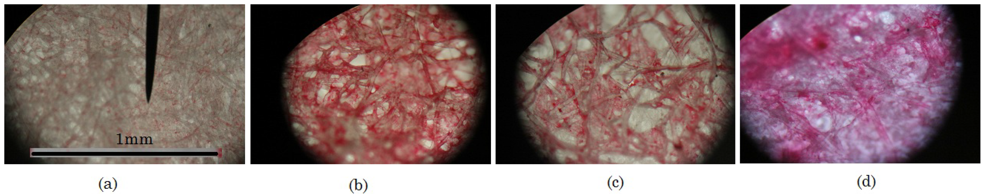
Our estimations of the porosity of the three different canvas types reveal that the void fractions for 90lb, 140lb and 140 lb cold pressed are 0.489, 0.319 and 0.29, respectively, suggesting 30% to nearly 50% of the canvas being empty space. Figure 3a–c show the canvas under a microscope with the last one, Figure 3d showing regular uncoated printer paper under the same magnification for comparison. All the surfaces have been stained with water color paint to highlight surface features. The images reveal substantial coarseness of the surfaces, especially in cases (a)–(c), when compared to plain paper and the porous nature of the canvas, even at such relatively low levels of magnification.
3. Results
The effective diameter of each splash was measured in centimeters, approximated by the largest width of the splash. The effective radius for each droplet was repeatedly measured continuously over time intervals of the order of a minute from the time of impact to the equilibrium state when the paint eventually dried on the paper (see Figure 4). Figure 5 depicts the evolution of the effective radius of the splash as a function of time. In particular, the figure shows a representative image of the impact of: height of droplet, temperature of the canvas, surface roughness of the canvas and viscosity of the paints upon this saturating curve. One can clearly see the impact of some these parameters more strongly than others from the figures. The effective radius of the paint is most affected by the paint type and nature of canvas (Figure 5c,d) which can be attributed to the varying frictional forces caused by the different pigment concentration of the paints and surface roughness of the canvas, respectively. The temperature of the canvas (Figure 5b) also shows interesting trends in the initial phase when surface characteristics are different. However, the true impact of all the parameters can be procured only by means of some more rigorous statistical means. Statistical analyses were conducted for the 46 different cases that were studied and correlations between the size of splash and the various control parameters are best determined using these tools. The statistical correlations are discussed below in Section 5, but, in the rest of this section, we discuss some other specific quantitative features, drawing upon similar work in the literature on slightly different systems.
As also noted in [24], we only observe two broad categories of splashing, namely deposition and prompt splashing due to the rapid absorption of much of the paint into the canvas upon contact. Within these categories, we identified distinct patterns in our experiments, which are classified into four sub-categories: (i) symmetric or circular patterns; (ii) splash pattern with a visible inner stamp; (iii) splash with strong radial fingering patterns; and (iv) satellite droplets. In Table 2 below, we explain the qualitative impact of the experimental parameters upon the appearance and strength of these splash patterns which are also shown in Figure 6. This is also further investigated in our statistical analysis section. In the table, the symbol ↑ indicates that the control parameter has an increasing effect upon the strength/magnitude/existence of that particular pattern while the symbol ↓ indicates the reverse.
Rioboo et al. [25] break down the deposition of paint on a dry surface into two phases: kinetic and actual, with the former displaying a radial growth , where r is the effective radius of the splash and t, is time. Such a profile is also observed in other studies concerning droplet splashes on liquid surfaces [26]. However, the value of the exponent is seen to vary in some other studies between – [27,28] which is attributed to the interaction of adjacent splashes. In our experiments, we also fit a power law function , to verify the radial growth rate of the splashes (see Figure 7). On average, over all the experiments performed, the average values of the fit parameters are and , with an average fit correlation . However, if the data is analyzed in terms of the freezing period of the canvas, we observe a distinctly different value of ; (i) in the case when the canvas is not frozen, , (ii) when the canvas is frozen for 5 min and (iii) when the canvas is frozen for 30 min, . In the current study, we therefore hypothesize the existence of three phases: (i) initial absorption, (ii) kinetic and (iii) actual. The initial absorption phase, which does not exist in the previous experiments, could potentially leave a relatively smaller volume of the droplet to spread. This would suggest a short kinetic phase which is dominated by capillary forces resulting in a slower growth rate. The relatively low value of our own exponent can be attributed to such an initial absorption phase.
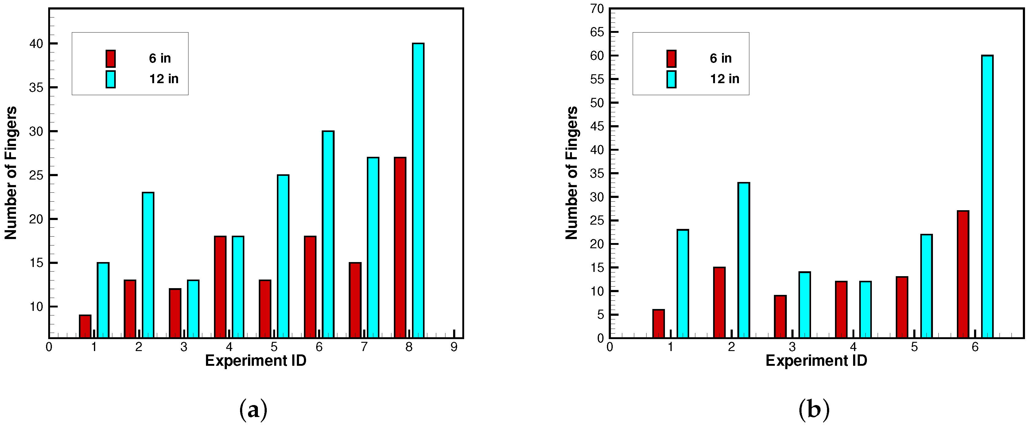
Following the work of Marmanis and Thoroddsen [24], we estimate the “number of fingers” as a function of height for various cases that show clear fingering patterns. As in [24], “...everything that resembles a finger, no matter how short...” is regarded a finger. The exact number of fingers however, is difficult to determine and the numbers reported must be realized to be approximate. Figure 8 depicts some sample cases of our analysis, which shows the count for the two different heights considered in this study ( and ) and two different paints (Permanent Rose and Prussian Blue). Clearly, in both cases, the height, or impact velocity is directly related to the number of fingers (also noted in [24]). In addition, the viscosity of the paint is inversely related to the number of fingers seen from comparing the two graphs Figure 8a,b. Other potential factors are more difficult to identify directly from the count and are dealt with in the following Section 5.
4. Fractal Dimension
The fractal analysis of drip paintings has become a research area of widespread interest in the past two decades [2,3,29]. The “organic” paintings of Jackson Pollock, in particular, have been identified as having a unique fractal signature. As a result, Taylor et al. [29] have claimed that the fractal dimension can be used as a means to identify artists and expose fakes, a claim which is contested by some [30]. However, this controversial issue aside, the fractal dimensional analysis of art is an interesting issue in itself. Furthermore, fractal patterns have also found unique and interesting applications such as in the field of environmental psychology, for therapeutic purposes (see [31] and references therein).
The method of box counting was implemented to approximate the fractal dimension of each painting. To estimate a two-dimensional fractal, a grid of boxes, each with a horizontal and vertical dimension of , , is superimposed over an image and the total number of boxes, , that are needed to cover the image are counted. At any given value of m, the fractal dimension, or Hausdorff dimension, is then approximated by . This procedure is repeated as , thus , the dimension of the figure. A Matlab based code was used to perform this computation. Consequently, a limit must be imposed on m to prevent from becoming infinitesimally small and infinitely large so as to yield a value equal to zero, and thus an indeterminate logarithmic ratio. Test images with known fractal dimension were used to determine the accuracy of the Matlab code. A numerical analysis of fractal dimension versus number of boxes graphically demonstrates an ideal box-count number around 200. At box-count numbers greater than about 400, the fractal dimension diverges from the target value because the number of boxes covering the image, , becomes negligible in comparison to the total number of boxes, , just as an object under a microscope might become blurry even though the lens gets closer and closer to a slide.
The photographs were saved in ‘JPG’ format, loaded into Matlab which converted a color image into a binary data array to produce a black and white figure (see Figure 9) which could then be analyzed with the box count method. Benchmark tests for the fractal dimension were performed (see Table 3) on several well known patterns such as Sierpinski triangle, Koch snowflake and Golden dragon [32]. Convergence studies were also conducted for box counts ranging from 25–500. Maximum error in our fractal dimension computation was about 0.09% when compared with their known dimensions.
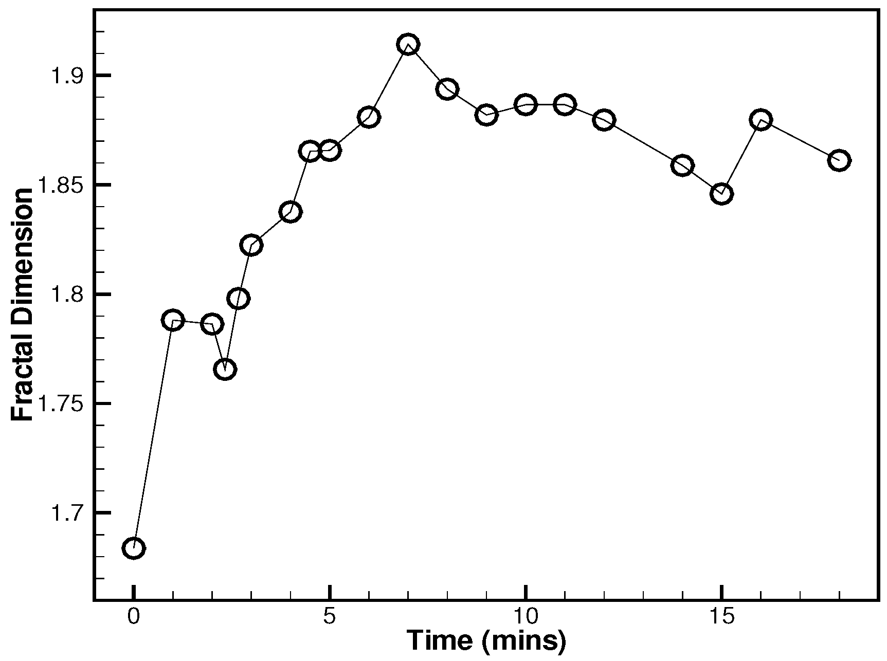
The time evolution of the fractal dimension was also computed and shows a similar overall profile to the effective radius. Figure 10 shows a sample curve corresponding to the images in Figure 4. However, this curve does not display a power-law correlation. The factors affecting the fractal dimension are discussed in the following section.
5. Statistical Analysis
We first modeled the relationship between scaled radius and the predictor variables: temperature (1 = unfrozen, 2 = frozen 5 min, 3 = frozen 30 min), height (1 = 6" and 2 = 12"), time, viscosity (1 = Permanent Rose, 2 = Prussian Blue and 3 = Sepia), type of paper (1 = canson 90 lb, 2 = arches 140 lb rough, 3 = arches 140 lb cold press) and the volume (1 = medicine dropper and 2 = straw), where time is the only continuous variable and all the others are treated as categorical variables. The fitted model result is given in Table A1 in the appendix. Further ANOVA analysis showed that all the predictors are significant predictors to the scaled radius. Based on Table A1, we can see that frozen 30 min significantly decreases the scaled radius compared to unfrozen temperature (p-value = 0), but frozen 5 min is not significantly different from unfrozen temperature. Height at 12" significantly increases the scaled radius compared to height at 6". With time increasing, it significantly increases the scaled radius. The normality and constant assumption of this multiple regression are met through residual plot check.
We then modeled how the same set of covariates affect certain specific patterns (termed hole pattern 1 and hole pattern 2). We create a binary variable for hole pattern 1 which corresponds to a prominent initial droplet stamp where paint has landed and dispersed, such as in Figure 6 (B2). We fit a logistic regression model using the covariates to explain the binary response variable hole pattern 1. The fitted model is given in Table A2 in the appendix. Height, time, paper type and volume are significant predictors to the binary response hole pattern 1. Specifically, height at 12" increases the odds of hole pattern 1; longer time increases the odds of hole pattern 1; Using paper type 2 has higher odds of hole pattern 1 than using paper type 1; and volume 2 has lower odds of hole pattern 1 than volume 1.
We fit a similar logistic model with response variable hole pattern 2 (rheological settling paint pattern within boundary of initial droplet with no interior stamp, for example Figure 6 (A2)). The fitted model is given in Table A3 in the appendix. The result indicates that all predictors are significant except for height. Frozen at 30 min has higher odds of hole pattern 2 than unfrozen. However, frozen 5 min has no significant difference from unfrozen. Longer time increases the odds of hole pattern 2. Prussian Blue and Sepia both have significant higher odds of hole pattern 2 than Permanent Rose, Sepia has the highest odds of hole pattern 2 compared to the other two viscosity levels. Canson 90 LB has the higher odds of hole pattern 2 than arches 140 LB rough and arches 140 LB cold press. Volume 2 (Straw) has higher odds of hole pattern 2 than volume 1 (medicine dropper).
We then fit the fractal dimension with all the predictors. For each experiment, we recorded the last fractal dimension value. In total, there are 46 observed fractal dimension values. We fit a multiple regression model but find two outliers from the residual plot and normal Q-Q plot. We removed two outliers and refit the model. The final result is given in Table A4 in the appendix. The result indicates temperature frozen at 30 min significantly reduces the fractal dimension value compared to unfrozen. Prussian Blue and Sepia significantly reduce the fractal dimension value compared to Permanent Rose. The residual against the fitted plot (see Figure 11a) and the normal Q-Q plot (see Figure 11b) indicate that the model assumptions are met and the inference obtained from this model are valid.
6. Conclusions
In summary, our experimental investigation of drop patterns of watercolors on canvas held at different temperatures, reveals patterns which depend upon material properties of the paint, canvas and also on the impact velocity and the temperature and wetting properties of the canvas. The radial growth pattern of the splash from the time of impact to equilibrium, achieved upon evaporation and settling, is qualitatively similar to that seen in previous studies, but the growth rate can vary between 0.1–0.47, depending upon the level of freezing of the canvas. The range of and puts this study in a well studied part of the experimental phase, which has been looked at before; however, there have been no previous studies on the effects of temperature and wetting on canvas in quite the same physical context.
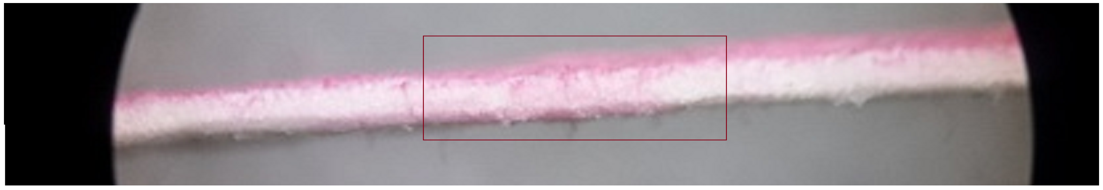
Figure 12 gives a qualitative idea of paint absorption which appears to be the greatest at the impact point and caused by the penetration of paint into depths of the wet canvas during first impact (referred to here as “initial absorption”). Details of the absorption process were not pursued in this study which has focused on the long term pattern evolution. However, we do recognize this to be an important aspect of the fluid dynamics involved here which will be investigated in our follow-up work. We also recognize that the absorption of paint into the canvas might also continue to occur post impact when the surface is in liquid state. Therefore, in principle, the overall dynamics could be characterized by the competition of not only and , but also perhaps by something additional such the Blake number, , which characterizes flows through porous media. Here, U is the flow speed, D is the characteristic length, ρ is the density, μ refers to dynamic viscosity and ϵ is the void fraction. In addition, non-Newtonian effects arising from the pigment concentration could also play an important role especially during the impact phase when shear stresses on the droplet are a maximum, making this a truly complex problem. Based on the material and flow parameters of this study, the overall values of B range from 394–2155 and shows sensitivity to the canvas, paint type and release height of droplet.
To qualitatively understand the effect of canvas porosity, we took a few images of the cross sectional slice of a droplet splash stain done about 5 min after the experiment, when the paint had not had a chance to evaporate. The image was obtained with a confocal microscope set at a magnification of about 300. The Figure 12 reveals some penetration, inferred from the pinkish hue of the paint at the center, i.e., the impact point, with not much absorption (at least not at this scale) elsewhere in the observed time. We therefore believe that while absorption might play some role at the early stages of the spread and paint penetration might continue to play a small role at later times as well. Therefore, the phenomenon still maintains the same overall properties as in the case of non-porous surface. In the case of 30 min canvas freezing, the surface is frozen and stays as such for several minutes past impact reducing the absorption time. Therefore, in this case, viscous and capillary regimes could dominate the absorption phase. Absorption dynamics appears to occur in two extremes of time scales: (a) the very short time impact scale where the maximum penetration is likely to occur and (b) the very long time scales where slow diffusion into the canvas occurs in the liquid-post-molten state of the canvas. Both these phases need further investigation.
We identify specific properties/patterns emerging in our experiments and a rigorous statistical analysis validates the qualitative observations, discussed in Table 2. A box count analysis of the images reveals that the splashes display fractal structure. The fractal dimension of the observed patterns are analyzed and contrasted with each other, revealing significant correlations to the environmental and material factors in this study. The fingering patterns observed in some of the experiments are seen to strongly correlate to the impact speed of the droplets and also the freezing temperature and the wetting of the canvas.
Overall, a thorough analysis of the physics of water color image on canvas can be extremely beneficial to watercolor artists to help render more controlled artistic works. Paint droplets on a substrate frozen for 30 min often produce a branch structure similar to microscopic blood vessels, after thawing for two to five minutes. Refreezing a painting at this moment may then permit the pigment to settle into the paper in this formation and allow for the emergence of new paint patterns not only for creative exploration but also for further scientific analysis. The beauty of watercolor painting lies in the complex flow of water along with the physical processes and the chemical reactions that occur within a singular pigment and between different paints. The nature of water allows pigment to open up and become translucent. The technique of wet-on-wet paint-canvas interaction is certainly not the only way to approach watercolor painting; wet-on-dry, dry-on-dry are equally valid methods, but wet paper makes for more vibrant colors. By freezing the paper, however, new and different patterns, e.g., fingering, branching, and confined sedimentation, became possible, which would otherwise quickly disperse and be a fleeting moment in the lifespan of the painting process.
The current study is only the first step in our understanding the physics of watercolor painting. Several interesting key questions remain including the effect of brush (shear stresses) on canvas and surface tension of paints. A more rigorous analysis of impact velocity is also desired. In addition, while a very complicated task, a theoretical/numerical analysis of the problem is also necessary for us to really appreciate the underlying physics. There have been some attempts at providing analytical explanations for the drop impact and spreading of liquids on solid surfaces [11,33,34]. These previous studies have incorporated Newtonian and non-Newtonian aspects of the liquids and also considered the effect of drying of the liquid. In the future, with the inclusion of absorption, these models could be considered towards application to our problem. Several of these ideas are either currently being pursued or will be taken up in our future, ongoing work on this subject.
Acknowledgments
We thank the editor for this invitation to the special issue. Our sincere thanks also to the reviewers for their very helpful comments and for raising interesting questions. The authors also thank Dirk Vanderklein for his help with obtaining the microscope images.
Author Contributions
Authors David Baron and Ashwin Vaidya designed and conducted the study. Haiyan Su performed the statistical analysis of the data.
Conflicts of Interest
The authors declare no conflict of interest.
Appendix A. Tables of Statistical Data

| Estimate | Std. Error | t Value | Pr(>|t|) | |
|---|---|---|---|---|
| (Intercept) | 5.5634 | 0.2156 | 25.81 | 0.0000 |
| factor(Temp)2 | 0.1926 | 0.1931 | 1.00 | 0.3188 |
| factor(Temp)3 | –1.8528 | 0.1841 | –10.06 | 0.0000 |
| factor(Height)2 | 0.2908 | 0.1398 | 2.08 | 0.0378 |
| Time | 0.1579 | 0.0088 | 17.89 | 0.0000 |
| factor(Viscosity)2 | –2.3478 | 0.1580 | –14.86 | 0.0000 |
| factor(Viscosity)3 | 0.7302 | 0.2721 | 2.68 | 0.0074 |
| factor(Paper)2 | 0.8153 | 0.1941 | 4.20 | 0.0000 |
| factor(Paper)3 | –0.4384 | 0.2769 | –1.58 | 0.1138 |
| factor(Volume)2 | 0.5852 | 0.1895 | 3.09 | 0.0021 |
| Estimate | Std. Error | z Value | Pr(>|z|) | |
|---|---|---|---|---|
| (Intercept) | –26.6447 | 1457.5012 | –0.02 | 0.9854 |
| factor(Temp)2 | 20.1488 | 1457.5009 | 0.01 | 0.9890 |
| factor(Temp)3 | 24.0557 | 1457.5010 | 0.02 | 0.9868 |
| factor(Height)2 | 1.0877 | 0.3406 | 3.19 | 0.0014 |
| Time | 0.3074 | 0.0365 | 8.42 | 0.0000 |
| factor(Viscosity)2 | –28.0664 | 1122.4010 | –0.03 | 0.9801 |
| factor(Viscosity)3 | –20.9046 | 2602.5289 | –0.01 | 0.9936 |
| factor(Paper)2 | 2.2046 | 0.4948 | 4.46 | 0.0000 |
| factor(Paper)3 | 0.5124 | 0.4571 | 1.12 | 0.2623 |
| factor(Volume)2 | –2.8894 | 0.5487 | –5.27 | 0.0000 |
| Estimate | Std. Error | z Value | Pr(>|z|) | |
|---|---|---|---|---|
| (Intercept) | –0.8532 | 0.2482 | –3.44 | 0.0006 |
| factor(Temp)2 | 0.0944 | 0.2309 | 0.41 | 0.6827 |
| factor(Temp)3 | 1.3492 | 0.2220 | 6.08 | 0.0000 |
| factor(Height)2 | –0.2046 | 0.1654 | –1.24 | 0.2161 |
| Time | 0.0035 | 0.0101 | 0.35 | 0.7289 |
| factor(Viscosity)2 | 1.3398 | 0.1847 | 7.25 | 0.0000 |
| factor(Viscosity)3 | 3.6557 | 0.5041 | 7.25 | 0.0000 |
| factor(Paper)2 | –1.2459 | 0.2277 | –5.47 | 0.0000 |
| factor(Paper)3 | –1.2640 | 0.3389 | –3.73 | 0.0002 |
| factor(Volume)2 | 0.8644 | 0.2167 | 3.99 | 0.0001 |
| Estimate | Std. Error | t Value | Pr(>|t|) | |
|---|---|---|---|---|
| (Intercept) | 1.8432 | 0.0537 | 34.35 | 0.0000 |
| factor(Temp)2 | –0.0329 | 0.0297 | –1.11 | 0.2762 |
| factor(Temp)3 | –0.0720 | 0.0303 | –2.38 | 0.0232 |
| factor(Height)2 | –0.0126 | 0.0240 | –0.53 | 0.6027 |
| Time | 0.0004 | 0.0021 | 0.18 | 0.8553 |
| factor(Viscosity)2 | –0.0582 | 0.0269 | –2.16 | 0.0377 |
| factor(Viscosity)3 | –0.1247 | 0.0483 | –2.58 | 0.0144 |
| factor(Paper)2 | 0.0035 | 0.0414 | 0.08 | 0.9338 |
| factor(Paper)3 | 0.0774 | 0.0476 | 1.63 | 0.1134 |
| factor(Volume)2 | 0.0359 | 0.0337 | 1.06 | 0.2947 |
References
- Lane, R. Images from the Floating World, The Japanese Print; Oxford University Press: Oxford, UK, 1978. [Google Scholar]
- Taylor, R.; Micolich, A.P.; Jonas, D. The construction of Jackson Pollock’s fractal drip paintings. Leonardo 2002, 203–207. [Google Scholar] [CrossRef]
- Taylor, R.P.; Micolich, A.P.; Jonas, D. Fractal Analysis of Pollock Drip Paintings. Nature 1999, 399, 422. [Google Scholar] [CrossRef]
- Hercynzki, A.; Cernuschi, C.; Mahadevan, L. Painting with drops, jets and sheets. Phys. Today 2011, 2011, 31–36. [Google Scholar]
- Worthington, A.M. A Study of Splashes; Longmans: London, UK, 1908; p. 129. [Google Scholar]
- Josserand, C.; Thoroddsen, S.T. Drop Impact on a Solid Surface. Annu. Rev. Fluid Mech. 2016, 48, 365–391. [Google Scholar] [CrossRef]
- Sefiane, K. Patterns from drying drops. Adv. Colloid Interface Sci. 2014, 206, 372–381. [Google Scholar] [CrossRef] [PubMed]
- Yarin, A.L. Drop Impact Dynamics: Splashing, Spreading, Receding, Bouncing. Ann. Rev. Fluid Mech. 2006, 38, 159–192. [Google Scholar] [CrossRef]
- Rioboo, R.; Tropea, C.; Marengo, M. Outcomes from a drop impact on solid surfaces. At. Sprays 2001, 11, 155–165. [Google Scholar]
- Bartolo, D.; Narcy, G.; Boudaoud, A.; Bonn, D. Dynamics of Non-Newtonian Droplets. Phys. Rev. Lett. 2007, 99, 174502. [Google Scholar] [CrossRef] [PubMed]
- Li-Hua, L.; Forterre, Y. Drop impact of yield-stress fluids. J. Fluid Mech. 2009, 632, 301–327. [Google Scholar]
- Marston, J.O.; Mansoor, M.M.; Thoroddsen, S.T. Impact of granular drops. Phys. Rev. E 2013, 88, 010201. [Google Scholar] [CrossRef] [PubMed]
- Nicolas, M. Spreading of a drop of neutrally buoyant suspension. J. Fluid Mech. 2005, 545, 271–280. [Google Scholar] [CrossRef]
- Peters, I.R.; Xu, Q.; Jaeger, H.M. Splashing onset in dense suspensions. Phys. Rev. Lett. 2013, 111, 028301. [Google Scholar] [CrossRef] [PubMed]
- Guemas, M.; Marin, A.G.; Lohse, D. Drop impact experiments of non-Newtonian liquids on micro-structured surfaces. Soft Matter 2012, 8, 10725–10731. [Google Scholar] [CrossRef]
- Mysels, K.J. Visual Art: The role of capillarity and rheological properties in painting. Leonardo 1981, 13, 22–27. [Google Scholar] [CrossRef]
- Lagubeau, G.; Fontelos, M.A.; Josserand, C.; Maurel, A.; Pagneux, V.; Petitjeans, P. Spreading dynamics of drop impacts. J. Fluid Mech. 2012, 713, 50–60. [Google Scholar] [CrossRef]
- How Watercolor Paints Are Made. Available online: http://www.handprint.com/HP/WCL/pigmt1.html (accessed on 15 December 2015).
- Blair, G.W.S. Rheology and Painting. Leonardo 1969, 2, 51–53. [Google Scholar] [CrossRef]
- Li, X.; Zhang, H.; Fang, Y.; Al-Assaf, S.; Phillips, G.O.; Nishinari, K. Rheological Properties of Gum Arabic Solution: The Effect of Arabinogalactan Protein Complex (AGP). In Gum Arabic; Kennedy, J.F., Phillips, G.O., Williams, P.A., Eds.; Royal Society of Chemistry: London, UK, 2011. [Google Scholar]
- Vernon-Carter, E.J.; Sherman, P. Rheological properties and applications of mesquite tree (Prosopis juliflora) gum. 1. Rheological properties of aqueous mesquite gum solutions. J. Text. Stud. 1980, 11, 339–349. [Google Scholar] [CrossRef]
- Lopez-Franco, Y.L.; Gooycolea, F.M.; Lizardi-Mendoza, J. Gum of Prosopis/Acacia Species; Ramawat, K.G., Merillon, J.-M., Eds.; Springer International Publishing: Cham, Switzerland, 2015. [Google Scholar]
- De Marsily, G. Quantitative Hydrogeology; Academic Press Inc.: Orlando, FL, USA, 1986. [Google Scholar]
- Marmanis, H.; Thoroddsen, S.T. Scaling of the fingering pattern of an impacting drop. Phys. Fluids 1996, 8, 1344–1346. [Google Scholar] [CrossRef]
- Rioboo, R.; Marengo, M.; Tropea, C. Time evolution of a liquid drop impact onto solid, dry surfaces. Expts Fluids 2002, 33, 112–124. [Google Scholar]
- Yarin, A.L.; Weiss, D.A. Impact of drops on solid surfaces: self-similar capillary waves, and splashing as a new type of kinematic discontinuity. J. Fluid Mech. 1995, 283, 141–173. [Google Scholar] [CrossRef]
- Cossali, G.E.; Coghe, A.; Marengo, M. The impact of a single drop on a wetted solid surface. Exp. Fluids 1997, 22, 463–472. [Google Scholar] [CrossRef]
- Sivakumar, D.; Tropea, C. Splashing impact of a spray onto a liquid film. Phys. Fluids 2002, 14, L85–L88. [Google Scholar] [CrossRef]
- Taylor, R.P.; Guzmana, R.; Martina, T.P.; Halla, G.D.R.; Micolichb, A.P.; Jonasb, D.; Scannella, B.C.; Fairbanksa, M.S.; Marlowa, C.A. Authenticating Pollock Paintings Using Fractal Geometry. Pattern Recognit. Lett. 2007, 28, 695. [Google Scholar] [CrossRef]
- Jones-Smith, K.; Mathur, H.; Krauss, L.M. Drip paintings and fractal analysis. Phys. Rev. E 2009, 79. [Google Scholar] [CrossRef] [PubMed]
- Joye, Y. Some reflections on the relevance of fractals for art therapy. Arts Psychother. 2006, 33, 143–147. [Google Scholar] [CrossRef]
- Lesmior-Gordon, N. Introducing Fractal Geometry; Icon Books Ltd.: Duxford, UK, 2006; p. 176. [Google Scholar]
- Howison, S.D.; Moriarty, J.A.; Terrill, E.L.; Wilson, S.K. A mathematical model for drying paint layers. J. Eng. Math. 1997, 32, 377–394. [Google Scholar] [CrossRef]
- Kim, H.Y.; Chun, J.H. The recoiling of liquid droplets upon collision with solid surfaces. Phys. Fluids 2001, 13, 643–659. [Google Scholar] [CrossRef]
Figure 1.
Experimental setup.

Figure 2.
Temperature of the canvas as a function of time for all three cases. The dashed lines point to the times when the canvas surface appears to be in molten liquid state.
Figure 2.
Temperature of the canvas as a function of time for all three cases. The dashed lines point to the times when the canvas surface appears to be in molten liquid state.
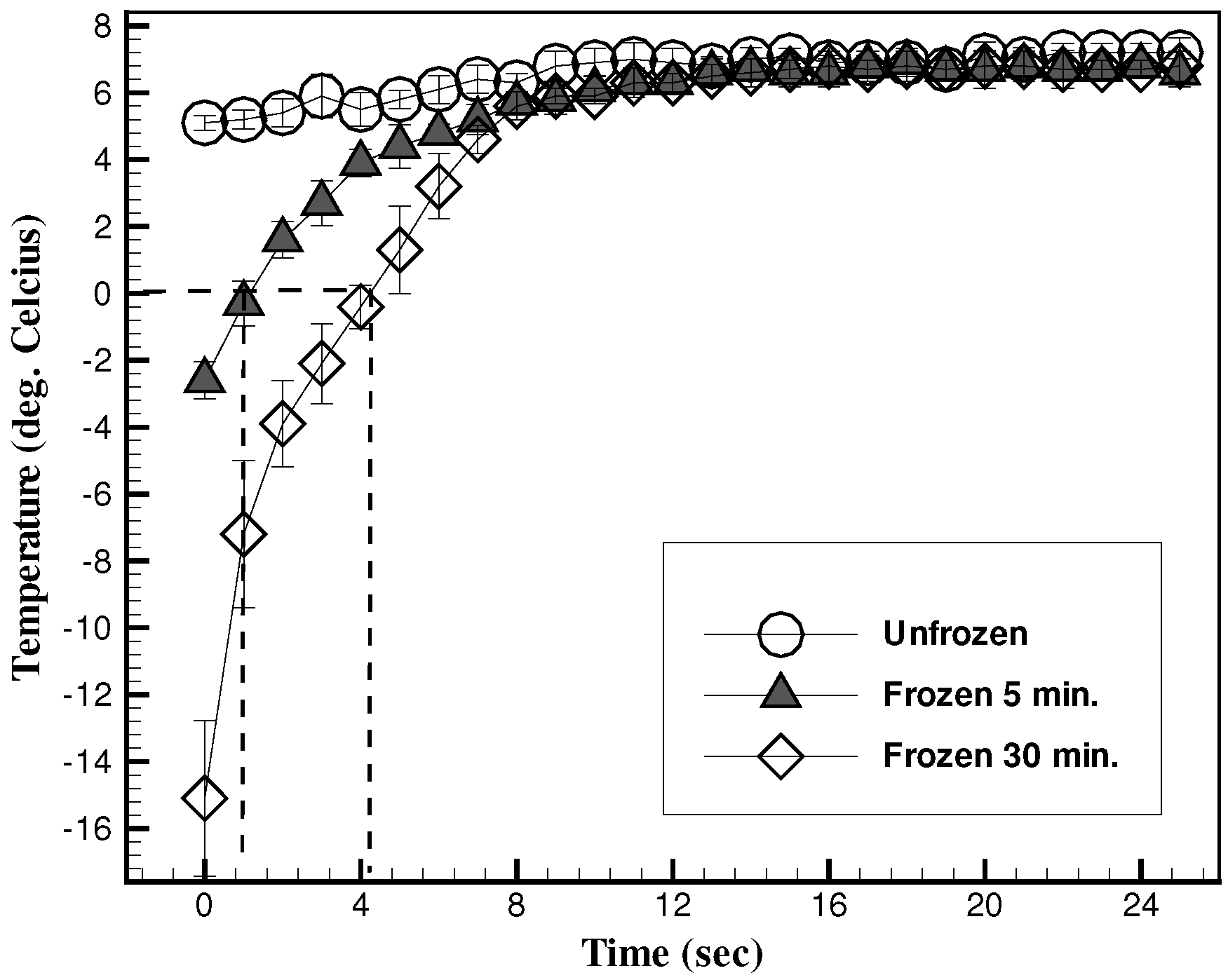
Figure 3.
Closeup view of the three canvases used in this study showing their surface features and porous nature. The pictures were taken with a Leica CME microscope (Meyer Instruments, Houston, TX, USA) at magnification of 100×. Images (a)–(c) correspond to 90 lb, 140 lb and 140 lb cold pressed canvas, respectively. The image (d) is of stained, uncoated printing paper at the same magnification.

Figure 4.
A time sequence of the splash of Permanent Rose on canvas.
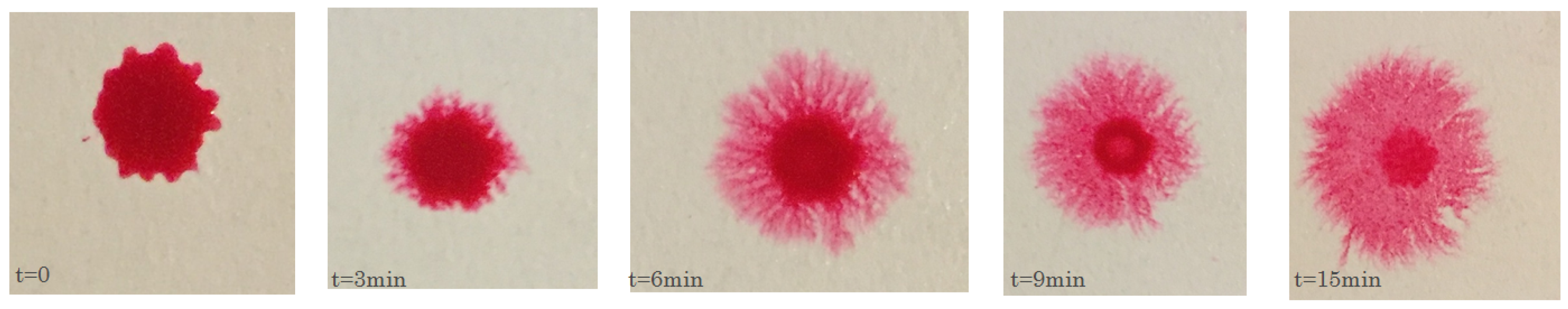
Figure 5.
The effective radius of the splash as a function of time showing the effect of (a) height of droplet; (b) the temperature of the canvas; (c) the viscosity of paint; and (d) the type of canvas used.
Figure 5.
The effective radius of the splash as a function of time showing the effect of (a) height of droplet; (b) the temperature of the canvas; (c) the viscosity of paint; and (d) the type of canvas used.
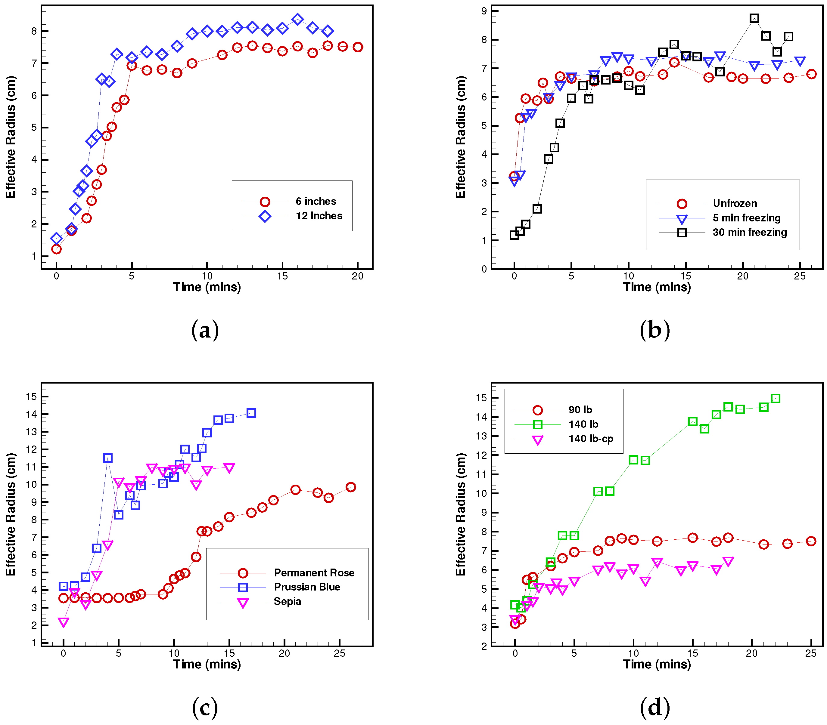
Figure 6.
Examples of the four distinct splash patterns seen in our experiments. A single splash can contain one or more of these patterns. The images are organized in pairs, with the first image (X1, where ), immediately upon impact and the final image (X2) are the images at the final times, at equilibrium.
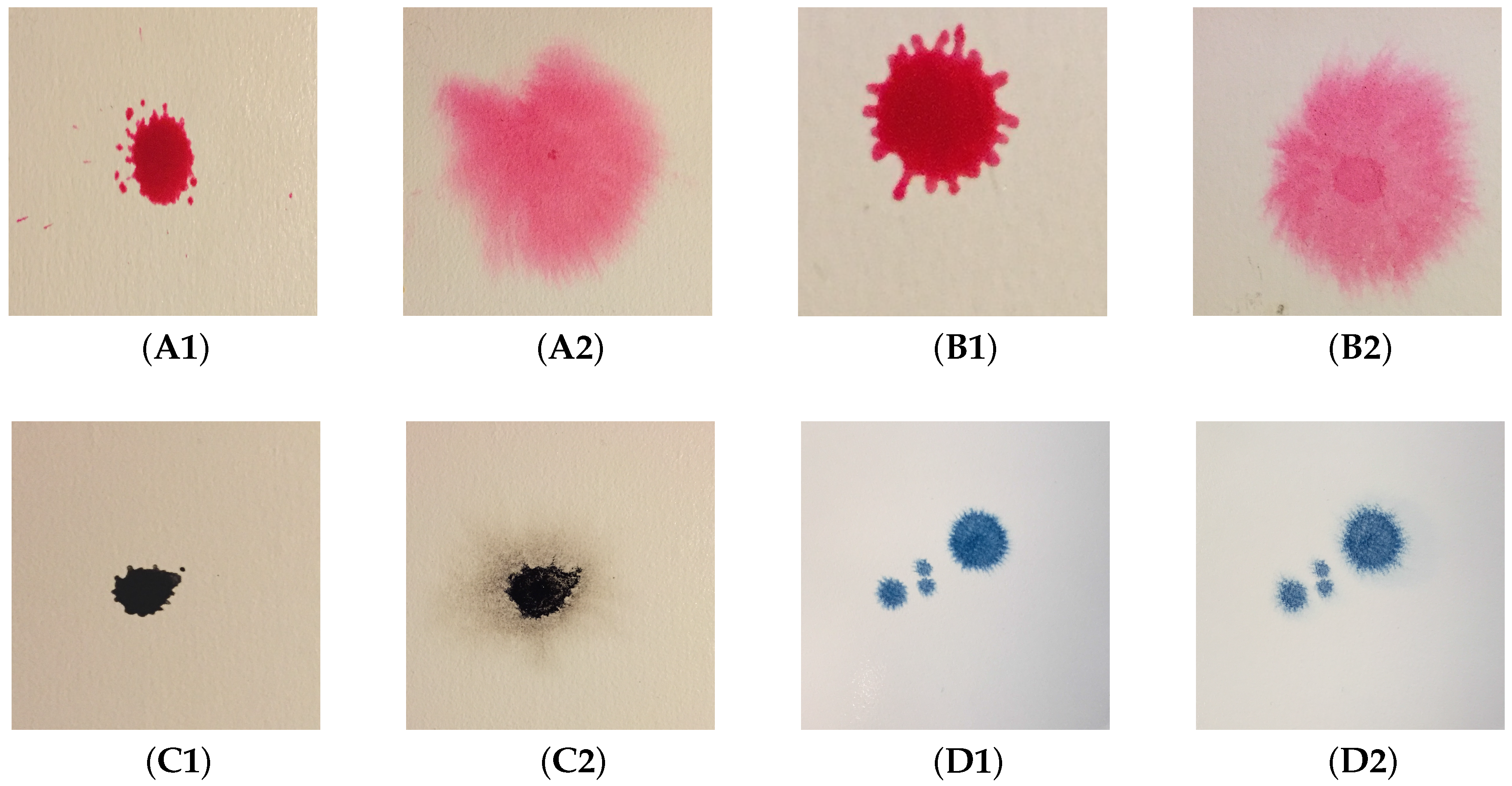
Figure 7.
The graph shows the evolution of the effective radius of the splash with time. A power law fit to the data is also shown, with an exponent value of 0.13, which is much smaller than those seen in other kinds of splashes.
Figure 7.
The graph shows the evolution of the effective radius of the splash with time. A power law fit to the data is also shown, with an exponent value of 0.13, which is much smaller than those seen in other kinds of splashes.
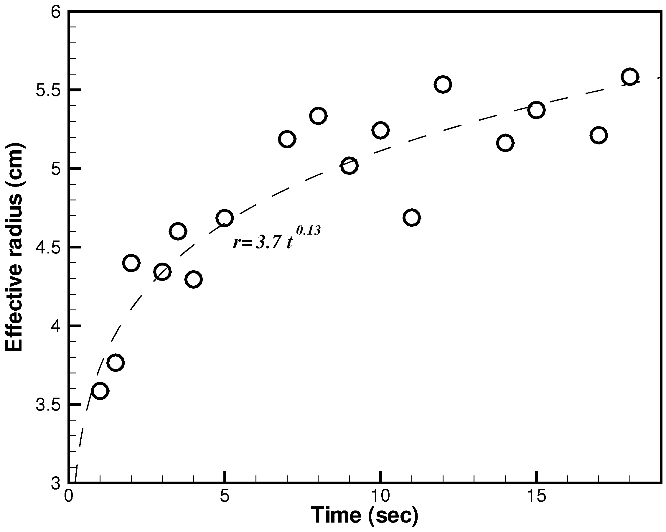
Figure 8.
Number of fingers as a function of height of release or impact velocity. Figure (a) shows the results for Permanent Rose and figure (b) shows the count for Prussian Blue. The x-axis represents different experimental cases where fingering was observed.
Figure 8.
Number of fingers as a function of height of release or impact velocity. Figure (a) shows the results for Permanent Rose and figure (b) shows the count for Prussian Blue. The x-axis represents different experimental cases where fingering was observed.

Figure 9.
A black and white image of a splash.
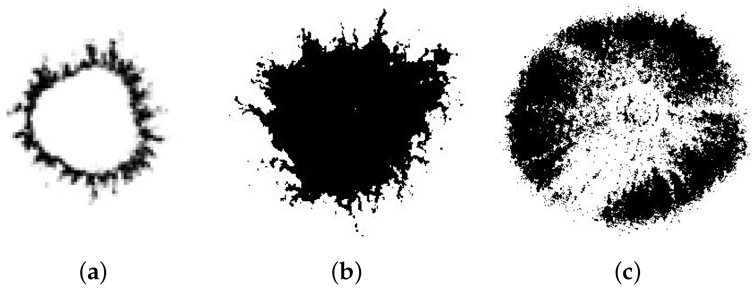
Figure 10.
Evolution of fractal dimension of a splash.

Figure 11.
Residual against fitted value plot for multiple regression model of fractal dimension. Normal Q-Q plot for multiple regression model of fractal dimension.
Figure 11.
Residual against fitted value plot for multiple regression model of fractal dimension. Normal Q-Q plot for multiple regression model of fractal dimension.
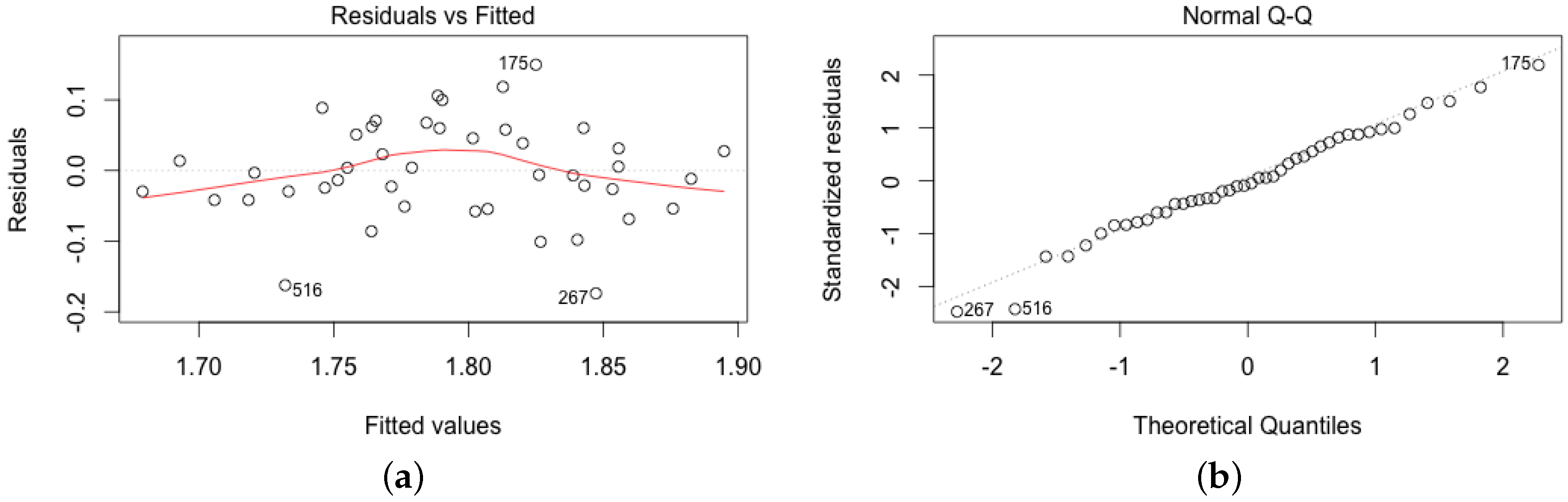
Figure 12.
Cross sectional image of canvas showing absorption and penetration of paint through canvas around the droplet impact point.
Figure 12.
Cross sectional image of canvas showing absorption and penetration of paint through canvas around the droplet impact point.

| Viscosity | Permanent Rose | Prussian Blue | Sepia |
|---|---|---|---|
| Average Viscosity (dPa-s) | 0.0257 | 0.0132 | 0.0098 |
| Std. Dev. | 0.0085 | 0.008 | 0.0071 |
Table 2.
Repeated patterns observed in our experiments are analyzed for their qualitative dependence upon canvas roughness, paint viscosity, height(or impact speed) and temperature of canvas.
| Property | Symmetric/Circular | Visible Inner Stamp | Radial Fingering | Satellites |
|---|---|---|---|---|
| Increase in... | ||||
| Height | ↓ | - | ↑ | ↑ |
| Paper Roughness | ↓ | ↓ | ↓ | |
| Paint Viscosity | - | ↑ | ↓ | - |
| Freezing | ↑ | ↑ | - | - |
| Temperature | Permanent Rose | Prussian Blue | Sepia |
|---|---|---|---|
| Unfrozen (6in) | 1.637 | 1.832 | 1.826 |
| Frozen 30 min (6in) | 1.975 | 1.570 | 1.707 |
| Unfrozen (12in) | 1.822 | 1.820 | 1.738 |
| Frozen 30 min (12in) | 1.931 | 1.722 | 1.650 |
© 2016 by the authors; licensee MDPI, Basel, Switzerland. This article is an open access article distributed under the terms and conditions of the Creative Commons Attribution license ( http://creativecommons.org/licenses/by/4.0/).
Share and Cite
MDPI and ACS Style
Baron, D.; Su, H.; Vaidya, A. Splash Dynamics of Paint on Dry, Wet, and Cooled Surfaces. Fluids 2016, 1, 12. https://doi.org/10.3390/fluids1020012
AMA Style
Baron D, Su H, Vaidya A. Splash Dynamics of Paint on Dry, Wet, and Cooled Surfaces. Fluids. 2016; 1(2):12. https://doi.org/10.3390/fluids1020012
Chicago/Turabian StyleBaron, David, Haiyan Su, and Ashwin Vaidya. 2016. "Splash Dynamics of Paint on Dry, Wet, and Cooled Surfaces" Fluids 1, no. 2: 12. https://doi.org/10.3390/fluids1020012