A Simple Stochastic Parameterization for Reduced Models of Multiscale Dynamics

Abstract

Multiscale dynamics are frequently present in real-world processes, such as the atmosphere-ocean and climate science. Because of time scale separation between a small set of slowly evolving variables and much larger set of rapidly changing variables, direct numerical simulations of such systems are difficult to carry out due to many dynamical variables and the need for an extremely small time discretization step to resolve fast dynamics. One of the common remedies for that is to approximate a multiscale dynamical systems by a closed approximate model for slow variables alone, which reduces the total effective dimension of the phase space of dynamics, as well as allows for a longer time discretization step. Recently, we developed a new method for constructing a deterministic reduced model of multiscale dynamics where coupling terms were parameterized via the Fluctuation-Dissipation theorem. In this work we further improve this previously developed method for deterministic reduced models of multiscale dynamics by introducing a new method for parameterizing slow-fast interactions through additive stochastic noise in a systematic fashion. For the two-scale Lorenz 96 system with linear coupling, we demonstrate that the new method is able to recover additional features of multiscale dynamics in a stochastically forced reduced model, which the previously developed deterministic method could not reproduce.

1. Introduction

Multiscale dynamics are common in applications of contemporary science, such as geophysical science and climate change prediction [1,2,3,4,5,6,7]. Multiscale dynamics are typically characterized by the time and space scale separation of patterns of motion, with fewer slowly evolving variables and much larger set of faster evolving variables. This time-space scale separation often made direct numerical computation of the dynamics on the slow time scale quite difficult in real-world applications, which led to the development of multiscale computational methods [8,9]. These methods make use of the averaging formalism [10,11,12] to allow for large time discretization steps for the computation of the slow part of the dynamics. However, in very large systems with many fast variables even these methods are computationally expensive.

As a different alternative to direct numerical simulation of the complete multiscale model with all variables, it has long been recognized that, if a closed simplified model for the slow variables alone was available, one could use this closed slow-variable model instead to simulate the statistics of the slow variables. In order to derive such a reduced model, one usually represents the process as a general two-scale dynamical system of the form

$$\frac{\mathrm{d}x}{\mathrm{d}t}=F(x,y)\frac{\mathrm{d}y}{\mathrm{d}t}=\frac{1}{\epsilon }G(x,y)$$

(1)

where $x\in {\mathbb{R}}^{N_x}$ and $y\in {\mathbb{R}}^{N_y}$ are the state vectors, and F and G are nonlinear differentiable functions. The scaling parameter $\epsilon \ll 1$ is used to separate the time scales in Equation (1) into slow (that is, x), and fast (that is, y). The scale separation parameter ε above is introduced for convenience of presentation, because, as shown below, the method developed here does not require its explicit presence to function. Besides, often real-world processes do not have any distinct time-scale separation parameters, and the fast and slow variables are known empirically from observations.

Under the assumption of “infinitely fast” y-variables, one writes the reduced averaged system for slow variables alone as

$$\frac{\mathrm{d}\overline{x}}{\mathrm{d}t}=\overline{F}(\overline{x})\overline{F}(\overline{x})={\int }_{{\mathbb{R}}^{N_y}}F(\overline{x},y)\mathrm{d}{\mu }_{\overline{x}}(y)$$

(2)

where ${\mu }_{\overline{x}}$ is the invariant distribution measure of the uncoupled fast dynamics where $\overline{x}$ is a fixed parameter:

$$\frac{\mathrm{d}z}{\mathrm{d}t}=G(\overline{x},z)$$

(3)

Under the assumption of ergodic ${\mu }_{\overline{x}}$, the measure integral in Equation (2) can be replaced with the time average along a single trajectory $z_{\overline{x}}(t)$ of Equation (3) for specified parameter $\overline{x}$:

$$\overline{F}(\overline{x})=\underset{T\to \infty }{lim}\frac{1}{T}{\int }_0^{T}F(\overline{x},z_{\overline{x}}(t))\mathrm{d}t$$

(4)

From Equations (2)–(4), it is clear that the computation of the averaged function $\overline{F}(\overline{x})$ is not a simple task; in fact, it is rarely available explicitly (except for some special cases where either the invariant distribution measure ${\mu }_{\overline{x}}$ or the solution $z_{\overline{x}}(t)$ are known as explicit formulas). A good example of the system where the invariant distribution measure is known explicitly is the Ornstein-Uhlenbeck process [13]; the invariant distribution measure of the Ornstein-Uhlenbeck process is a Gaussian distribution with explicitly known mean state and covariance matrix. Because of this convenient property, the Ornstein-Uhlenbeck process is popular in the area of stochastic modeling of geophysical and other real-world processes.

The “upgrade” from the deterministic reduced model in Equation (2) is a stochastic model of the form

$$\mathrm{d}\overline{x}=\overline{F}(\overline{x})\mathrm{d}t+\sigma (\overline{x})\mathrm{d}{W}_t$$

(5)

where $W_t$ is a Wiener process, and $\sigma (\overline{x})$ is a matrix. This model was suggested in [2], and is referred to as the “nonlinear diffusion approximation” in [14]. It is the correct homogenization approximation in the case where the vector field G of the fast y-dynamics in Equation (1) does not depend on x [15,16,17], whereas in the case of a fully coupled multiscale dynamics an additional deterministic term of order ε appears in Equation (5) [14,18]. Here we choose to omit this extra term due to, first, difficulty in its numerical computation, and, second, its relatively small contribution.

The stochastic reduced model in Equation (5) is generally considered to be more advantageous to the deterministic reduced model in Equation (2), because the random noise can be used to parameterize “noise-like” influence from fast variables onto slow dynamics, which is entirely lacking in the deterministic reduced model in Equation (2). Sometimes, deterministic reduced models of atmospheric processes fail to adequately represent atmospheric variability; it is thought that a significant portion of atmospheric variability is essentially noise-like, and fitting it with deterministic forcing terms does not seem to be a good way to produce an adequate approximation. Additionally, the deterministic slow dynamics in Equation (2) tend to produce the attractor of the slow dynamics with significantly lower dimension than that for the full two-scale dynamics in Equation (1), especially for weakly chaotic slow variables. At the same time, if the stochastic forcing in Equation (5) is strong enough, it should “diffuse” the invariant manifolds of Equation (2), thus inflating the dimension of the set containing limiting dynamics.

Nonetheless, in many applications, the reduced dynamics of the deterministic type in Equation (2) or stochastic type in Equation (5) are not available explicitly. As a result, numerous approximate closure schemes were developed for multiscale dynamical systems [9,19,20,21,22,23], which are all based on the averaging/homogenization principle over the fast variables [10,11,12]. Some of the methods (such as those in [20,21,22,23]) replace the fast nonlinear dynamics with suitable stochastic processes [24], discontinuous Markov jump processes [25], or conditional Markov chains [19], while others [9] provide direct closure by suitable tabulation and curve fitting. Reduced stochastic dynamics were used to model global circulation patterns [26,27,28,29,30], and large-scale features of tropical convection [31,32]. However, it seems that all these approaches require either extensive computations to produce a closed model (for example,[9,19] require multiple simulations of fast variables alone with different fixed states of slow variables), or somewhat ad hoc determination of closure coefficients by matching areas under the time correlation functions [20,21,22,23]. Another interesting method was recently developed in [33], however, again, somewhat ad hoc approach was used to compute the closure (namely, slow variables of a multiscale system were treated as if their dynamics were generated by a running average of an Ornstein-Uhlenbeck process). Recently, a stochastic parameterization of a reduced dynamics was used in [34] for a low-order coupled atmosphere-ocean model.

In two recent works [35,36] the author developed a relatively simple and straightforward method of constructing the deterministic reduced model for slow variables of a multiscale model with nonlinear and multiplicative coupling, which required only a single computation of certain statistics of the fast dynamics with a fixed state of the slow variables, located in the region where the slow dynamics usually evolve. The method was based on the first-order Taylor expansion of the averaged coupling term with respect to the slow variables, which was computed using the Fluctuation-Dissipation theorem [37,38,39,40,41,42,43,44]. It was demonstrated through the computations with the appropriately rescaled two-scale Lorenz 96 model [45,46] that, with nonlinear and multiplicative coupling in both slow and fast variables, the developed reduced model produced good approximation to the statistics of the full two-scale Lorenz 96 model. Among the advantages of the developed method were its simplicity and explicit formulation. Additionally, existing zero-order models of this kind for the Earth’s atmosphere (such as the T21 barotropic model [42,47,48]) can be retrofitted with the new deterministic correction term emerging from the theory in [35].

In the current work, we introduce a method for computing a consistent approximation of the form in Equation (5) to the multiscale dynamics in Equation (1). The method is aimed at stochastic parameterization of general complex nonlinear multiscale dynamics with many variables, and has essentially the same implementation restrictions as the method for deterministic reduced models we developed previously in [35,36]. We test the new method on the two-scale Lorenz 96 model, where only the linear part of the coupling is enabled for the simplicity of presentation. We demonstrate through direct numerical simulations that the new method generally improves properties of statistics of the reduced model, and, in particular, the injection of random noise into a deterministic reduced model can make it both more or less chaotic and mixing, depending on the difference between the dynamical regimes of the reduced and full two-scale models.

We must mention, however, that a formally more accurate stochastic reduced model can be obtained from Equation (5) by adding a small deterministic correction term [14,18]. However, this additional deterministic correction term is given as a statistical correlation of the slow vector field with its own Jacobian, which is difficult to implement and expensive to compute numerically. The main motivation for the current work, however, is to test a relatively simple and inexpensive stochastic extension to the already available deterministic reduced model [35,36], which can be used to simplify a general nonlinear multiscale dynamics. Due to this reason, we chose to omit the small deterministic correction term from [14,18].

The manuscript is organized as follows. In Section 2 we present the general description of the new method, following the homogenization theory of [49]. In Section 3 we lay out the step-by-step computational implementation of the new method for a general two-scale dynamical system with linear coupling between the slow and fast variables, which does not contain any explicit time-scale separation parameters. In Section 4 we test the new method on the two-scale Lorenz 96 model in a range of dynamical regimes with varying chaos, mixing, and time scale separation between the slow and fast variables. Section 5 summarizes the results of this work.

2. General Description of the Method

Here we introduce a new method for the stochastic correction of the form in Equation (5) for the deterministic reduced model in Equation (2). To derive the method, we use the theoretical framework similar to that applied to homogenization problems in [49]. To simplify presentation, we assume that the deterministic averaged function $\overline{F}(\overline{x})$ from Equation (2) is already available, either as an explicit formula, or as an approximation we developed previously in [35,36]. Below, x is used to denote the state of the slow variables from the multiscale system in Equation (1), while $\overline{x}$ denotes the state of the slow variables from the deterministic reduced model in Equation (2). The difference between x and $\overline{x}$ is denoted as $q=x-\overline{x}$. Then, one can rewrite the multiscale system in Equation (1) in the new variables as

$$\frac{\mathrm{d}\overline{x}}{\mathrm{d}t}=\overline{F}(\overline{x})$$

(6a)

$$\frac{\mathrm{d}q}{\mathrm{d}t}=F(\overline{x}+q,y)-\overline{F}(\overline{x})$$

(6b)

$$\frac{\mathrm{d}y}{\mathrm{d}t}=\frac{1}{\epsilon }G(\overline{x}+q,y)$$

(6c)

What we see above is that the first equation is already a closed system from Equation (2), and given a suitable approximation for $\overline{F}$ from [35,36], it can be solved on its own. Thus, $\overline{x}(t)$ can be treated as a given function of time. This, in effect, leaves q and y as the unknown variables, and Equation (6a) can be dropped. Now, the idea is to apply the homogenization formalism to q, obtaining $\overline{q}$ as the next order correction to $\overline{x}$. In this situation, the reduced model for $\overline{q}$ should be derived as the Itô diffusion process of the corresponding backward Kolmogorov equation restricted to slow time scale (see [49] for details), under the condition that q (and, therefore, $\mathrm{d}q/\mathrm{d}t$) in Equations (6b)–(6c) is $O(\epsilon )$. To do that, first we bring the time scale of q in Equations (6b)–(6c) to $O(1)$ by rescaling the time t as $\tau =\epsilon t$. For the rescaled time τ, from Equations (6b)–(6c) we obtain

$$\frac{\mathrm{d}q}{\mathrm{d}\tau }=\frac{1}{\epsilon }\left[F(\overline{x}+q,y)-\overline{F}(\overline{x})\right]$$

(7a)

$$\frac{\mathrm{d}y}{\mathrm{d}\tau }=\frac{1}{{\epsilon }^2}G(\overline{x}+q,y)$$

(7b)

Above, the evolution equation for $\overline{x}$ is no longer needed, as $\overline{x}(\tau )$ is a given function of rescaled time τ. Now we write the backward Kolmogorov equation for Equations (7a)–(7b). For that, let $v(\tau ,{\tau }^{\prime },\overline{x},q,y)$, ${\tau }^{\prime }\ge \tau$, be the value of a test function $h(q({\tau }^{\prime }),y({\tau }^{\prime }))$, given $q(\tau )=q$, and $y(\tau )=y$. Then, $v(\tau ,{\tau }^{\prime },\overline{x},q,y)$ obeys the following backward Kolmogorov equation (for reference, see, for example, [50]):

$$\frac{\partial v(\tau ,{\tau }^{\prime },\overline{x},q,y)}{\partial \tau }=\left[\frac{1}{{\epsilon }^2}G(\overline{x}+q,y)·{\nabla }_y+\frac{1}{\epsilon }\left[F(\overline{x}+q,y)-\overline{F}(\overline{x})\right]·{\nabla }_q\right]v(\tau ,{\tau }^{\prime },\overline{x},q,y)$$

(8)

Below, we drop the ${\tau }^{\prime }$-dependence from v as it is of no consequence to what is presented. Observe that the terms in the backward Kolmogorov equation above are multiplied by different powers of ε, which leads to the perturbation expansion of the solution $v(\tau ,\overline{x},q,y)$ in powers of ε, and derivation of the backward Kolmogorov equation for the term which has the lowest power of ε in the closed form. Then, its corresponding Itô diffusion process will be the evolution equation for $\mathrm{d}\overline{q}/\mathrm{d}t$, as long as $\overline{q}$ is small enough.

The expansion of $v(\tau ,\overline{x},q,y)$ in powers of ε is

$$v=v_0+\epsilon v_1+{\epsilon }^2{v}_2+\dots$$

(9)

Plugging the expansion above back into the Kolmogorov equation in Equation (8) and collecting the terms with matching powers of ε, we obtain the following relations for each power of ε:

$$G(\overline{x}+q,y)·{\nabla }_y{v}_0=0\text{for}{\epsilon }^{-2}$$

(10a)

$$G(\overline{x}+q,y)·{\nabla }_y{v}_1=-\left[F(\overline{x}+q,y)-\overline{F}(\overline{x})\right]·{\nabla }_q{v}_0\text{for}{\epsilon }^{-1}$$

(10b)

$$\frac{\partial v_0}{\partial \tau }=G(\overline{x}+q,y)·{\nabla }_y{v}_2+\left[F(\overline{x}+q,y)-\overline{F}(\overline{x})\right]·{\nabla }_q{v}_1\text{for}{\epsilon }^0$$

(10c)

Below we consider each of the relations above separately.

• Order ${\epsilon }^{-2}$. From the relation in Equation (10a) we determine that $v_0(\tau ,\overline{x},q,y)=v_0(\tau ,\overline{x},q)$, that is, $v_0$ does not depend on y.
• Order ${\epsilon }^{-1}$. Here we use the relation in Equation (10b) to express $v_1$ in terms of $v_0$. We denote the flow, generated by Equation (3), by ${\varphi }_{\overline{x}}^s$, so that ${\varphi }_{\overline{x}}^{s}y$ is the solution of Equation (3) forward in time s with the initial condition y, with the obvious identity

  $$\frac{\partial }{\partial s}{\varphi }_{\overline{x}+q}^{s}y=G(\overline{x}+q,{\varphi }_{\overline{x}+q}^{s}y)$$

  (11)

  Now, consider the integral

  $$\begin{array}{c}\hfill u(s,\overline{x},q,y)={\int }_s^{\infty }\left[F(\overline{x}+q,{\varphi }_{\overline{x}+q}^{r}y)-\overline{F}(\overline{x})\right]\mathrm{d}r·{\nabla }_q{v}_0=\\ \hfill ={\int }_0^{\infty }\left[F(\overline{x}+q,{\varphi }_{\overline{x}+q}^r({\varphi }_{\overline{x}+q}^{s}y))-\overline{F}(\overline{x})\right]\mathrm{d}r·{\nabla }_q{v}_0\end{array}$$

  (12)

  where the group property of ${\varphi }_{\overline{x}}^s$ is used in the second equality. Then, from the first identity in Equation (12), it follows that

  $${\left.\frac{\partial }{\partial s}u(s,\overline{x},q,y)\right|}_{s=0}=-\left[F(\overline{x}+q,y)-\overline{F}(\overline{x})\right]·{\nabla }_q{v}_0$$

  (13)

  and from the second identity in Equation (12) it follows that $u(s,\overline{x},q,y)$ is in fact an explicit function of ${\varphi }_{\overline{x}+q}^{s}y$, that is, $u(s,\overline{x},q,y)\equiv U(\overline{x},q,{\varphi }_{\overline{x}+q}^{s}y)$. However, any $U(\overline{x},q,{\varphi }_{\overline{x}+q}^{s}y)$ must obey the transport equation

  $$\begin{array}{c}\hfill \frac{\partial }{\partial s}U(\overline{x},q,{\varphi }_{\overline{x}+q}^{s}y)=\nabla U(\overline{x},q,{\varphi }_{\overline{x}+q}^{s}y)·\frac{\partial }{\partial s}{\varphi }_{\overline{x}+q}^{s}y=\\ \hfill =G(\overline{x}+q,{\varphi }_{\overline{x}+q}^{s}y)·\nabla U(\overline{x},q,{\varphi }_{\overline{x}+q}^{s}y)\end{array}$$

  (14)

  where the second identity is due to Equation (11), and which holds for any s including $s=0$. Combining Equations (13) and (14) at $s=0$, we obtain

  $$G(\overline{x}+q,y)·{\nabla }_{y}u(0,\overline{x},q,y)=-\left[F(\overline{x}+q,y)-\overline{F}(\overline{x})\right]·{\nabla }_q{v}_0$$

  (15)

  From the comparison with Equation (10b) it follows that $v_1=u(0,\overline{x},q,y)$, that is,

  $$v_1={\int }_0^{\infty }\left[F(\overline{x}+q,{\varphi }_{\overline{x}+q}^{s}y)-\overline{F}(\overline{x})\right]\mathrm{d}s·{\nabla }_q{v}_0.$$

  (16)
• Order ${\epsilon }^0$. Here observe that $v_0$ does not depend on y, as pointed out above. This means that the average of $v_0$ with respect to the invariant distribution measure ${\mu }_{\overline{x}+q}$ of Equation (3) is the identity operation, and the same holds for its τ-derivative. Then, averaging out Equation (10c) with respect to ${\mu }_{\overline{x}+q}$ yields,

  $$\begin{array}{cc}\hfill \frac{\partial v_0}{\partial \tau }& ={\int }_{{\mathbb{R}}^{N_y}}G(\overline{x}+q,y)·{\nabla }_y{v}_2\mathrm{d}{\mu }_{\overline{x}+q}(y)+\hfill \\ & +{\int }_{{\mathbb{R}}^{N_y}}\left[F(\overline{x}+q,y)-\overline{F}(\overline{x})\right]·{\nabla }_q{v}_1\mathrm{d}{\mu }_{\overline{x}+q}(y)\hfill \end{array}$$

  (17)

  For the first integral above we express the gradient term as a time derivative of the function along the flow (in the same way as above for $v_1$):

  $$G(\overline{x}+q,y)·{\nabla }_y{v}_2(\tau ,\overline{x},q,y)={\left.\frac{\partial }{\partial s}{v}_2(\tau ,\overline{x},q,{\varphi }_{\overline{x}+q}^{s}y)\right|}_{s=0}$$

  (18)

  The invariant distribution measure ${\mu }_{\overline{x}+q}$ preserves the averages of functions of ${\varphi }_{\overline{x}+q}^{s}y$:

  $${\int }_{{\mathbb{R}}^{N_y}}{v}_2(\tau ,q,{\varphi }_{\overline{x}+q}^{s}y)\mathrm{d}{\mu }_{\overline{x}+q}(y)=\text{constant, for all }s$$

  (19)

  This, in turn, results in

  $$\frac{\partial }{\partial s}{\int }_{{\mathbb{R}}^{N_y}}{v}_2(\tau ,\overline{x},q,{\varphi }_{\overline{x}+q}^{s}y)\mathrm{d}{\mu }_{\overline{x}+q}(y)=0,\text{for all }s,\text{ including }s=0$$

  (20)

  and, therefore,

  $$\frac{\partial v_0}{\partial \tau }={\int }_{{\mathbb{R}}^{N_y}}\left[F(\overline{x}+q,y)-\overline{F}(\overline{x})\right]·{\nabla }_q{v}_1\mathrm{d}{\mu }_{\overline{x}+q}(y)$$

  (21)

At this point, substituting the expression for $v_1$ from Equation (16), and rescaling time τ back to t yields

$$\frac{\partial v_0}{\partial t}=\left[Q(\overline{x}+q,\overline{x})·{\nabla }_q+\frac{1}{2}S(\overline{x}+q,\overline{x}):\left({\nabla }_q\otimes {\nabla }_q\right)\right]v_0$$

(22a)

$$Q(a,b)=\epsilon {\int }_0^{\infty }{\int }_{{\mathbb{R}}^{N_y}}\left(\frac{\partial }{\partial a}F(a,{\varphi }_a^{s}y)\right)\left[F(a,y)-\overline{F}(b)\right]\mathrm{d}{\mu }_a(y)\mathrm{d}s$$

(22b)

$$S(a,b)=2\epsilon \mathrm{Sym}{\int }_0^{\infty }{\int }_{{\mathbb{R}}^{N_y}}\left[F(a,{\varphi }_a^{s}y)-\overline{F}(b)\right]\otimes \left[F(a,y)-\overline{F}(b)\right]\mathrm{d}{\mu }_a(y)\mathrm{d}s$$

(22c)

where “:” denotes the Frobenius product of two matrices, and “$\mathrm{Sym}$” denotes the symmetric part of a matrix (the skew-symmetric part is canceled out by the Frobenius product with a symmetric matrix).

As a result, the next-order correction $\overline{q}$ to the averaged dynamics in Equation (2), generated by the backward Kolmogorov equation above, is given by the Itô diffusion process

$$\frac{\mathrm{d}\overline{x}}{\mathrm{d}t}=\overline{F}(\overline{x})$$

(23a)

$$\mathrm{d}\overline{q}=Q(\overline{x}+\overline{q},\overline{x})\mathrm{d}t+\sigma (\overline{x}+\overline{q},\overline{x})\mathrm{d}{W}_t$$

(23b)

as long as $\overline{q}$ is small enough. Above, $W_t$ is a K-dimensional Wiener process for some positive integer K, $Q(\overline{x}+\overline{q},\overline{x})$ is the $O(\epsilon )$ $N_y$-vector drift term, and $\sigma (\overline{x}+\overline{q},\overline{x})$ is the $O(\sqrt{\epsilon })$$N_y\times K$ stochastic diffusion matrix, given (non-uniquely) by

$$\sigma {\sigma }^T=S$$

(24)

Thus far, in Equations (23a)–(23b) we obtained the equations for two sets of variables, $\overline{x}$ and $\overline{q}$, while the evolution of the stochastic reduced dynamics for Equation (1) is given by the sum $(\overline{x}+\overline{q})$. However, what we actually need is an approximate reduced model for $(\overline{x}+\overline{q})$ directly. For that, we add Equations (23a) and (23b) to obtain

$$\begin{array}{cc}\hfill \mathrm{d}(\overline{x}+\overline{q})& =\overline{F}(\overline{x}+\overline{q})\mathrm{d}t+\sigma (\overline{x}+\overline{q},\overline{x}+\overline{q})\mathrm{d}{W}_t+\hfill \\ \hfill +& \left[\overline{F}(\overline{x})-\overline{F}(\overline{x}+\overline{q})+Q(\overline{x}+\overline{q},\overline{x})\right]\mathrm{d}t+\hfill \\ & +[\sigma (\overline{x}+\overline{q},\overline{x})-\sigma (\overline{x}+\overline{q},\overline{x}+\overline{q})]\mathrm{d}{W}_t\hfill \end{array}$$

(25)

Above, observe that the first term in the right-hand side is $O(1)$, the second term is $O(\sqrt{\epsilon })$, and the rest of the terms are $O(\epsilon )$ or higher (taking into account that $\overline{q}$ is $O(\epsilon )$). Additionally, the terms in the second and third line of Equation (25) are very difficult to compute in practice for complex nonlinear dynamics. Therefore, we delete the terms in the second and third lines from Equation (25), thus completely decoupling Equation (25) from Equations (23a)–(23b). Then, after replacing $(\overline{x}+\overline{q})\to \overline{x}$, we obtain the stochastic reduced model in Equation (5), where the diffusion matrix σ is computed according to Equations (22c) and (24) with $a=b=\overline{x}$ (further we denote $S(\overline{x})\equiv S(\overline{x},\overline{x})$).

Remark: $\sigma (\overline{x})$ Does not Depend on ε.

It is important to note that $S(\overline{x})$, and, therefore, $\sigma (\overline{x})$, do not in fact depend on ε. Indeed, observe that

$$\begin{array}{c}\hfill S(\overline{x})=2\epsilon \mathrm{Sym}{\int }_0^{\infty }{\int }_{{\mathbb{R}}^{N_y}}\left[F(\overline{x},{\varphi }_{\overline{x}}^{s}y)-\overline{F}(\overline{x})\right]\otimes \left[F(\overline{x},y)-\overline{F}(\overline{x})\right]\mathrm{d}{\mu }_{\overline{x}}(y)\mathrm{d}s=\\ \hfill =2\mathrm{Sym}{\int }_0^{\infty }{\int }_{{\mathbb{R}}^{N_y}}\left[F(\overline{x},{\varphi }_{\overline{x}}^{s/\epsilon }y)-\overline{F}(\overline{x})\right]\otimes \left[F(\overline{x},y)-\overline{F}(\overline{x})\right]\mathrm{d}{\mu }_{\overline{x}}(y)\mathrm{d}s\end{array}$$

(26)

where ${\varphi }_{\overline{x}}^{s/\epsilon }y$ is the solution of the fast dynamics from Equation (1) (with ${\epsilon }^{-1}$ still in front of $G(x,y)$) with $x=\overline{x}$ fixed as a constant parameter. Thus, there is no need to know what ε is to compute $S(\overline{x})$, and, in fact, ε does not have to be an explicit scaling parameter in the multiscale dynamics in Equation (1). This makes the new method practical in realistic applications, where time-scale difference might not be explicitly available in the form of a parameter.

3. Practical Implementation of the Reduced Stochastic Model For a General Multiscale Process With Linear Coupling

As formulated above in Section 2, the new method is applicable for a broad range of dynamical systems with general forms of coupling. However, for the clarity of presentation, we dedicate a separate section to the implementation of the developed method for a multiscale process with linear coupling. The linear coupling is the most basic form of coupling in physical processes, however, because of that it is also probably the most common form of coupling. Below we describe the complete step-by-step assembly of the reduced model, with both the deterministic and stochastic terms which parameterize coupling.

Here we consider the special setting of Equation (1) with linear coupling between x and y:

$$\frac{\mathrm{d}x}{\mathrm{d}t}=f(x)+L_{y}y\frac{\mathrm{d}y}{\mathrm{d}t}=g(y)+L_{x}x$$

(27)

where f and g are nonlinear vector functions of x and y, respectively, and $L_x$ and $L_y$ are constant matrices of suitable sizes. As before, x and y denote the slow and fast variables, respectively. However, one important distinction between Equation (27) and Equation (1) is that we no longer make use of the time scale separation parameter ε; here the assumption is that it is somehow known that x-variables are slow, and y-variables are fast, but no further information about time scale separation is available beyond that, and, in particular, no explicit time scale separation parameter is known. As before, we introduce the corresponding fast limiting system

$$\frac{\mathrm{d}z}{\mathrm{d}t}=g(z)+L_{x}x$$

(28)

with x specified as a constant parameter. It is easy to see that for the multiscale system with linear coupling in Equation (27), the matrix $S(\overline{x})$ from Equation (22c) is computed as the time-lag correlation matrix

$$S(\overline{x})=2L_y\mathrm{Sym}\left[{\int }_0^{\infty }{\int }_{{\mathbb{R}}^{N_y}}\left({\varphi }_{\overline{x}}^{s}y-\overline{z}(\overline{x})\right){\left(y-\overline{z}(\overline{x})\right)}^T\mathrm{d}{\mu }_{\overline{x}}(y)\mathrm{d}s\right]L_y^T$$

(29)

where ${\varphi }_{\overline{z}}^s$ is the solution of Equation (28), with x fixed at constant parameter $\overline{x}$, forward in time s from an initial condition y, and $\overline{z}(\overline{x})$ is the mean state of Equation (28). Before constructing the reduced model, we need realistic assumptions on what we can compute in the multiscale system in Equation (27), which we take directly from [35,36]:

• First, we are going to presume that the multiscale dynamical system in Equation (27) is not necessarily computable at will for arbitrarily long time intervals. The reason is that if it is possible, then the need for a reduced model becomes somewhat difficult to justify.
• Even if the full multiscale model is not computable at will, we still need some statistical information about it to formulate the reduced model. Here, we presume that some typical state $x^{*}$ of the slow variables x is available, such that the dynamics evolve in the proximity of $x^{*}$. For example, a rough estimate of the mean state of the slow variables of the full multiscale system can be taken as $x^{*}$, or a nearby state.
• We presume that the limiting fast dynamics in Equation (28) is computable beyond the mixing time scale, so that time averages of Equation (28) can be computed, at least for a single given value $x=x^{*}$.
• The assumptions above are the same as in [35,36], in order to ensure compatibility of the proposed stochastic reduced model method with what we have already developed in [35,36] for deterministic reduced models of multiscale dynamics with nonlinear and multiplicative coupling.

Under the above assumptions and the ergodicity hypothesis, we compute the mean state $\langle z\rangle$ and the time covariance matrix $C(\tau )$ from the long-term time series of the solution $z(t)$ of Equation (28) with fixed parameter $x=x^{*}$:

$$\langle z\rangle =\underset{T\to \infty }{lim}\frac{1}{T}{\int }_0^{T}z(t)\mathrm{d}t$$

(30a)

$$C(\tau )=\underset{T\to \infty }{lim}\frac{1}{T}{\int }_0^T\left(z(t+\tau )-\langle z\rangle \right){\left(z(t)-\langle z\rangle \right)}^T\mathrm{d}t$$

(30b)

$$\overline{C}={\int }_0^{\infty }C(\tau )\mathrm{d}\tau$$

(30c)

Then, we assemble the reduced stochastic model for Equation (27) in the explicit form as

$$\mathrm{d}\overline{x}=\left[f(\overline{x})+L_y\langle z\rangle +L_{y}R{L}_x(\overline{x}-x^{*})\right]\mathrm{d}t+\sigma \mathrm{d}{W}_t$$

(31)

where the constant terms R and σ are computed as

$$R=\overline{C}{C}^{-1}(0)$$

(32a)

$$\sigma {\sigma }^T=S=L_y\left(\overline{C}+{\overline{C}}^T\right)L_y^T$$

(32b)

Above, the deterministic part in Equation (31) is computed as described in [35] using the quasi-Gaussian linear response approximation [43], while the stochastic part is computed according to Equation (29) (where the measure average is replaced with the time average) with $\overline{x}=x^{*}$. Observe that the matrix σ will be computed only once, for the particular value $x^{*}$. That, in effect, makes it a constant matrix approximation to the exact $\sigma (\overline{x})$ from Equation (24), provided that the trajectory $\overline{x}(t)$ of the reduced model in Equation (31) is in the vicinity of $x^{*}$. This type of stochastic parameterization with a constant diffusion matrix is called the additive noise parameterization (as opposed to the multiplicative noise parameterization, where σ is a function of $\overline{x}$). In the future work, we plan to extend the method described here onto the multiplicative noise parameterization.

The Choice of σ.

Observe that σ is not determined uniquely by Equation (32b), as multiple decompositions of S into $\sigma {\sigma }^T$ are available (the Cholesky decomposition into the product of a lower-triangular matrix with its own transpose being one of the examples). Here we use the following algorithm to compute σ: first, solve the eigenvalue problem

$$SX=X\Lambda$$

(33)

where X is the matrix of eigenvectors, and Λ is the diagonal matrix of eigenvalues. Since S is symmetric and nonnegative-definite [49], then all eigenvalues in Λ are guaranteed to be positive, and all eigenvectors in X are guaranteed to be orthonormal (so that $X^{-1}=X^T$). Then, we compute σ as

$$\sigma =X{\Lambda }^{1/2}{X}^T$$

(34)

This method uniquely determines σ as a square, symmetric, and positive-definite diffusion matrix for the Wiener process $W_t$.

4. Computational Study: The Two-Scale Lorenz 96 Model With Linear Coupling

The test multiscale system used to study the new method of stochastic parameterization here is the rescaled two-scale Lorenz 96 system with linear coupling, previously used in [35] to study the deterministic reduced model parameterization. The Lorenz 96 system is given by

$${\dot{x}}_i=x_{i-1}(x_{i+1}-x_{i-2})+\frac{1}{{\beta }_x}(\overline{x}(x_{i+1}-x_{i-2})-x_i)+\frac{F_x-\overline{x}}{{\beta }_x^2}-\frac{{\lambda }_y}{J}\sum _{j=1}^J{y}_{i,j}$$

(35a)

$${\dot{y}}_{i,j}=\frac{1}{\epsilon }\left[y_{i,j+1}(y_{i,j-1}-y_{i,j+2})+\frac{1}{{\beta }_y}(\overline{y}(y_{i,j-1}-y_{i,j+2})-y_{i,j})+\frac{F_y-\overline{y}}{{\beta }_y^2}\right]+\frac{{\lambda }_x}{\epsilon }{x}_i$$

(35b)

with $1\le i\le N_x$ and $1\le j\le J$, such that $N_y=N_{x}J$. The model has periodic boundary conditions: $x_{i+N_x}=x_i$, $y_{i,j+J}=y_{i+1,j}$, and $y_{i+N_x,j}=y_{i,j}$. The parameter $\epsilon \ll 1$ sets the time scale separation between the slow variables $x_i$, and the fast variables $y_{i,j}$. The parameters $(\overline{x},{\beta }_x)$ and $(\overline{y},{\beta }_y)$ are the (mean, standard deviation) pairs for the corresponding uncoupled and unrescaled Lorenz models

$${\dot{x}}_i=x_{i-1}(x_{i+1}-x_{i-2})-x_i+F_x$$

(36a)

$${\dot{y}}_{i,j}=y_{i,j+1}(y_{i,j-1}-y_{i,j+2})-y_{i,j}+F_y$$

(36b)

with the same periodic boundary conditions. The rescaling above ensures that the Lorenz 96 model in Equations (35a)–(35b) has zero mean state and unit standard deviation for both slow and fast variables in the absence of coupling (${\lambda }_x={\lambda }_y=0$), and remain near these values when ${\lambda }_x$ and ${\lambda }_y$ are nonzero. The linear coupling above preserves the energy of the form

$$E=\frac{{\lambda }_x}{2}\sum _{i=1}^{N_x}{x}_i^2+\frac{\epsilon {\lambda }_y}{2J}\sum _{i=1}^{N_x}\sum _{j=1}^J{y}_{i,j}^2$$

(37)

Below we display the results of a numerical study of the stochastic reduced model for slow variables of multiscale dynamics, using the rescaled Lorenz system in Equations (35a)–(35b) as the test model. We compare the statistical properties of the slow variables for the four following systems:

• The complete rescaled Lorenz system from Equations (35a)–(35b);
• The stochastic reduced model from Equation (31);
• The deterministic reduced model obtained from Equation (31) by removing the stochastic forcing (this model was previously developed in [35]);
• The poor man’s version of Equation (31) with no stochastic forcing and the first-order linear deterministic correction term R set to zero (further referred to as the “zero-order” system, same as in [35]). This zero-order system represents the simplest reduced model with constant parameterization of coupling terms.

The fixed parameter $x^{*}$ for the computation of $\langle z\rangle$, R and σ was set to the long-term mean state $\langle x\rangle$ of the full multiscale model in Equations (35a)–(35b) (in computationally expensive models, a rough estimate could be used). Like in [35,36], for all computational statistical results presented below, the averaging time window $T_{av}$ equals 10000 time units.

Due to translational invariance of the studied models, the statistics are invariant with respect to the index shift for the variables $x_i$. For diagnostics, we monitor the following long-term statistical quantities of $x_i$:

• The distribution density functions, computed by bin-counting. A distribution density function gives the best information about the one-point statistics of $x_i$, as it shows the statistical distribution of $x_i$ in the phase space.
• The time auto-correlation functions $\langle x_i(t)x_i(t+s)\rangle$, where the time average is over t, normalized by the variance $\langle x_i^2\rangle$ (so that it always starts with 1).
• The time cross-correlation functions $\langle x_i(t)x_{i+1}(t+s)\rangle$, also normalized by the variance $\langle x_i^2\rangle$.
• The energy auto-correlation function

  $$K(s)=\frac{\langle x_i^2(t)x_i^2(t+s)\rangle }{{\langle x_i^2\rangle }^2+2{\langle x_i(t)x_i(t+s)\rangle }^2}$$

  This energy auto-correlation function measures the non-Gaussianity of the process (it is identically 1 for all s if the process is Gaussian, such as the Ornstein-Uhlenbeck process). For details, see [23].

The following dynamical regimes are studied:

• $N_x=20$, $J=4$ (so that $N_y=80$). Thus, the number of the fast variables is four times greater than the number of the slow variables.
• $\epsilon =0.01,0.1$. The time scale separation of two orders of magnitude ($\epsilon =0.01$) is consistent with typical real-world geophysical processes (for example, the annual and diurnal cycles of the Earth’s atmosphere). Also, in large-scale atmospheric processes the time scale separation between slow and fast variables can be weaker than that (for example, typical time scale of equatorial Kelvin waves is about 70 days, and that of Yanai waves is about 30 days, which is well in between the annual and diurnal cycles), so we additionally test the dynamical regimes with weak time scale separation $\epsilon =0.1$.
• ${\lambda }_x={\lambda }_y=0.3,0.35$. These values of coupling are chosen so that they are neither too weak, nor too strong (although 0.3 is weaker, and 0.35 is stronger). However, this small variation in coupling changes the dynamical regime in the slow variables between moderately ($\epsilon =0.3$) and weakly ($\epsilon =0.35$) chaotic and mixing, due to the suppression of chaos effect previously studied in [51].
• $F_x=6$. The slow forcing $F_x$ adjusts the chaos and mixing properties of the slow variables, and in this work it is set to a weak-to-moderate chaotic regime $F_x=6$. The reason for that is that it was found previously in [35] that in strongly chaotic and mixing regimes at slow variables there is not much of a difference between the multiscale dynamics and reduced models.
• $F_y=16$. The fast forcing adjusts the chaos and mixing properties of the fast variables. Here the value of $F_y$ is chosen so that the fast variables are strongly chaotic and mixing for $F_y=16$.

4.1. Moderate Mixing at Slow Variables With Weak Time Scale Separation

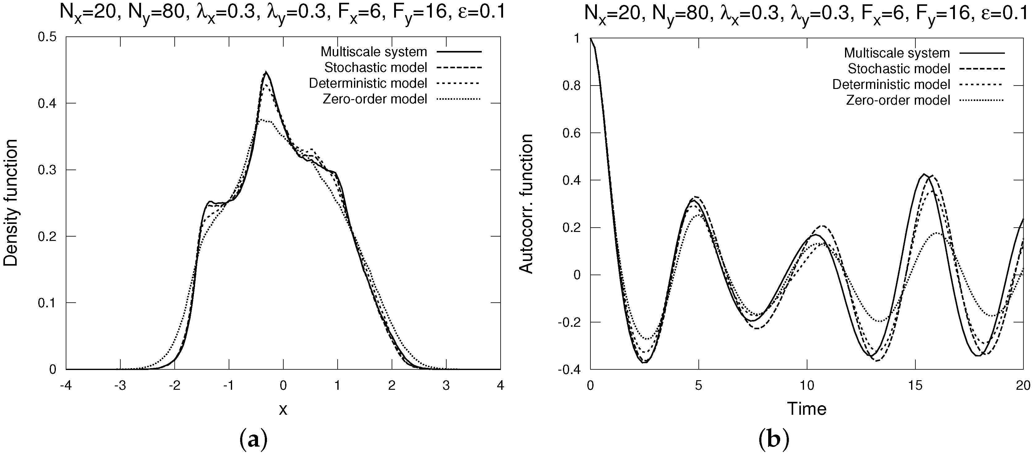
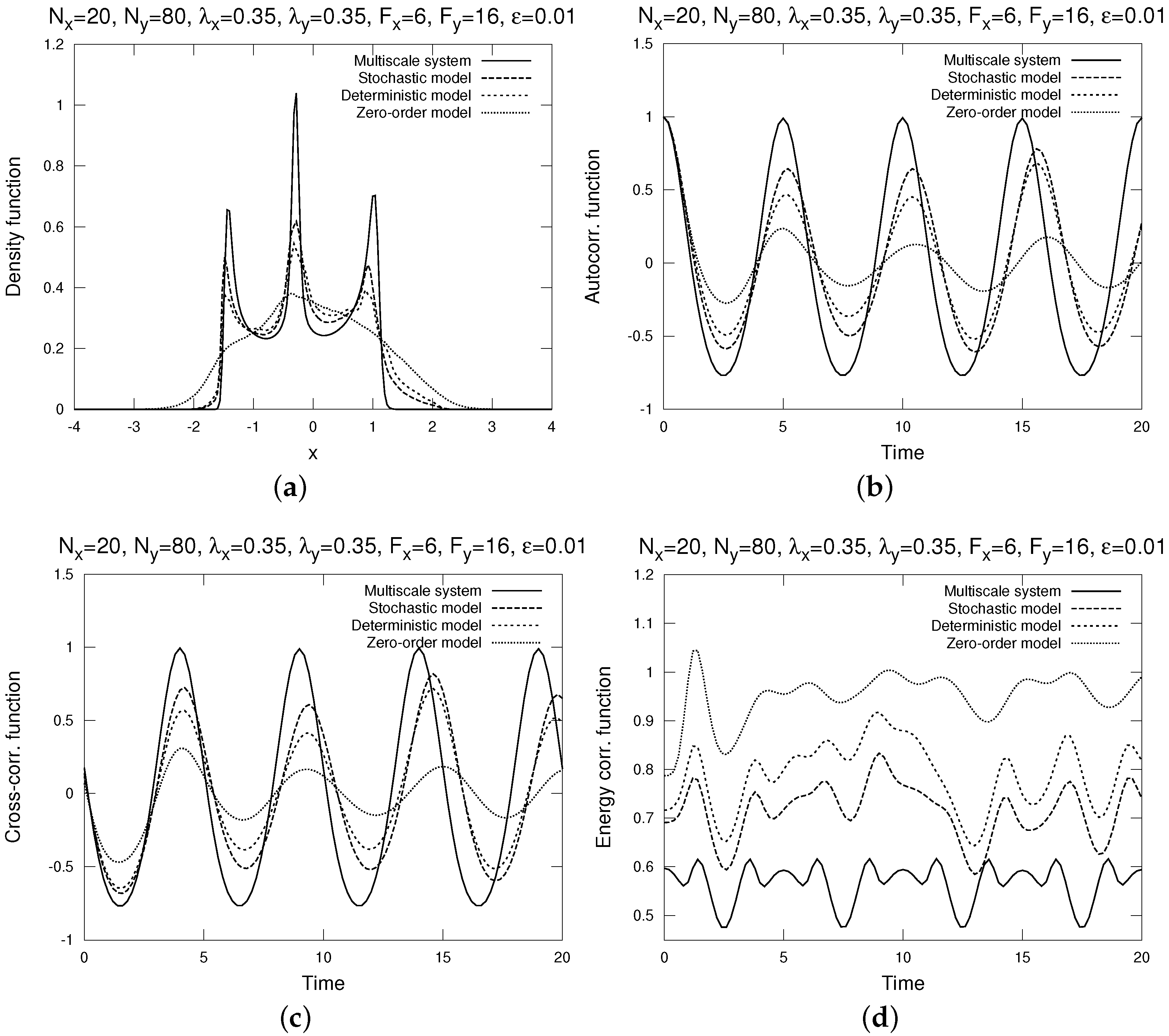
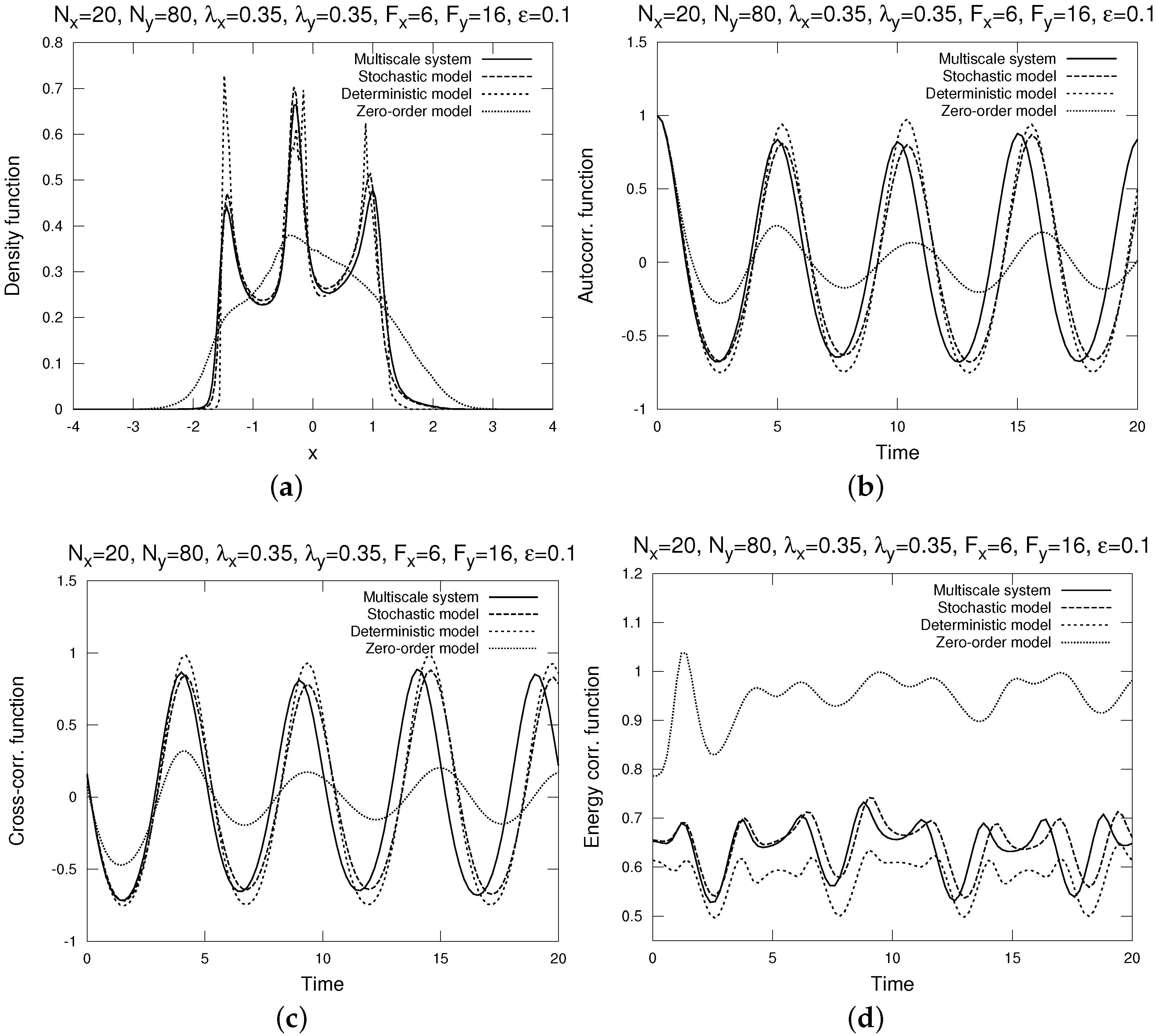
Here we present the comparison of different statistics for the dynamical regime with moderate chaos and mixing at slow variables (achieved by setting ${\lambda }_x={\lambda }_y=0.3$) and weak time scale separation (achieved by setting $\epsilon =0.1$). In Figure 1 we show the distribution density functions, time auto-correlation functions, time cross-correlation functions, and energy auto-correlation functions for the multiscale dynamics in Equations (35a)–(35b), and three different kinds of the reduced models: the new stochastic reduced model, the deterministic reduced model from [35], and the zero-order reduced model with constant parameterization of coupling terms (which is given for reference as a simplest/poorest form of parameterization). Observe that the difference between the new stochastic and deterministic models here are rather small, however, it does look like the additional stochastic term improves the statistics. In particular, the stochastic terms makes the distribution density more spiky towards the multiscale density, and appears to produce better fits for correlation functions. The probable reason why there is not much of a difference between the deterministic and stochastic reduced models is that the slow dynamics are not sufficiently weakly chaotic for the stochastic term to make a significant difference. Table 1 confirms that there is some improvement error-wise in the distribution density and energy auto-correlation, but no improvement in auto- and cross-correlations (probably due to oscillations getting out of sync with increased lag time).

Figure 1. (a) Distribution density function; (b) time auto-correlation function; (c) time cross-correlation function; (d) energy auto-correlation function. $F_x=6$, $F_y=16$, ${\lambda }_x={\lambda }_y=0.3$, $\epsilon =0.1$.

Figure 1. (a) Distribution density function; (b) time auto-correlation function; (c) time cross-correlation function; (d) energy auto-correlation function. $F_x=6$, $F_y=16$, ${\lambda }_x={\lambda }_y=0.3$, $\epsilon =0.1$.

Table 1. Relative errors between the slow variables of the full multiscale system, and different reduced models, computed for the plots in Figure 1. $F_x=6$, $F_y=16$, ${\lambda }_x={\lambda }_y=0.3$, $\epsilon =0.1$.

Rel. Error	Stochastic	Deterministic	Zero-Order
Density	$3.803\times {10}^{-3}$	$7.424\times {10}^{-3}$	$2.093\times {10}^{-2}$
Corr.	$0.1218$	$0.1152$	$0.1935$
Cross-corr.	$0.1297$	$0.1222$	$0.2118$
Energy corr.	$1.312\times {10}^{-2}$	$1.436\times {10}^{-2}$	$3.473\times {10}^{-2}$

Table 1. Relative errors between the slow variables of the full multiscale system, and different reduced models, computed for the plots in Figure 1. $F_x=6$, $F_y=16$, ${\lambda }_x={\lambda }_y=0.3$, $\epsilon =0.1$.

Rel. Error	Stochastic	Deterministic	Zero-Order
Density	$3.803\times {10}^{-3}$	$7.424\times {10}^{-3}$	$2.093\times {10}^{-2}$
Corr.	$0.1218$	$0.1152$	$0.1935$
Cross-corr.	$0.1297$	$0.1222$	$0.2118$
Energy corr.	$1.312\times {10}^{-2}$	$1.436\times {10}^{-2}$	$3.473\times {10}^{-2}$

4.2. Moderate Mixing at Slow Variables With Strong Time Scale Separation

Here we present the comparison of different statistics for the dynamical regime with moderate chaos and mixing at slow variables (achieved by setting ${\lambda }_x={\lambda }_y=0.3$) and strong time scale separation (achieved by setting $\epsilon =0.01$). In Figure 2 we show the distribution density functions, time auto-correlation functions, time cross-correlation functions, and energy auto-correlation functions for the multiscale dynamics in Equations (35a)–(35b), and three different kinds of the reduced models: the new stochastic reduced model, the deterministic reduced model from [35], and the zero-order reduced model with constant parameterization of coupling terms. Observe that the difference between the new stochastic and deterministic models here are even smaller than for the regime with weak time-scale separation, probably due to the fact that the contribution of the stochastic term scales as $\sqrt{\epsilon }$. However, again, it looks like the additional stochastic term improves the statistics somewhat. Table 2 show that there is some improvement error-wise in all presented statistics, but not enough to be discernible visually in Figure 2.

Table 2. Relative errors between the slow variables of the full multiscale system, and different reduced models, computed for the plots in Figure 2. $F_x=6$, $F_y=16$, ${\lambda }_x={\lambda }_y=0.3$, $\epsilon =0.01$.

Rel. Error	Stochastic	Deterministic	Zero-Order
Density	$8.105\times {10}^{-3}$	$1.048\times {10}^{-2}$	$2.233\times {10}^{-2}$
Corr.	$9.309\times {10}^{-2}$	$9.627\times {10}^{-2}$	$0.1923$
Cross-corr.	$9.57\times {10}^{-2}$	$9.99\times {10}^{-2}$	$0.2129$
Energy corr.	$9.042\times {10}^{-3}$	$1.209\times {10}^{-2}$	$2.776\times {10}^{-2}$

Table 2. Relative errors between the slow variables of the full multiscale system, and different reduced models, computed for the plots in Figure 2. $F_x=6$, $F_y=16$, ${\lambda }_x={\lambda }_y=0.3$, $\epsilon =0.01$.

Rel. Error	Stochastic	Deterministic	Zero-Order
Density	$8.105\times {10}^{-3}$	$1.048\times {10}^{-2}$	$2.233\times {10}^{-2}$
Corr.	$9.309\times {10}^{-2}$	$9.627\times {10}^{-2}$	$0.1923$
Cross-corr.	$9.57\times {10}^{-2}$	$9.99\times {10}^{-2}$	$0.2129$
Energy corr.	$9.042\times {10}^{-3}$	$1.209\times {10}^{-2}$	$2.776\times {10}^{-2}$

Figure 2. (a) Distribution density function; (b) time auto-correlation function; (c) time cross-correlation function; (d) energy auto-correlation function. $F_x=6$, $F_y=16$, ${\lambda }_x={\lambda }_y=0.3$, $\epsilon =0.01$.

Figure 2. (a) Distribution density function; (b) time auto-correlation function; (c) time cross-correlation function; (d) energy auto-correlation function. $F_x=6$, $F_y=16$, ${\lambda }_x={\lambda }_y=0.3$, $\epsilon =0.01$.

4.3. Weak Mixing at Slow Variables With Weak Time Scale Separation

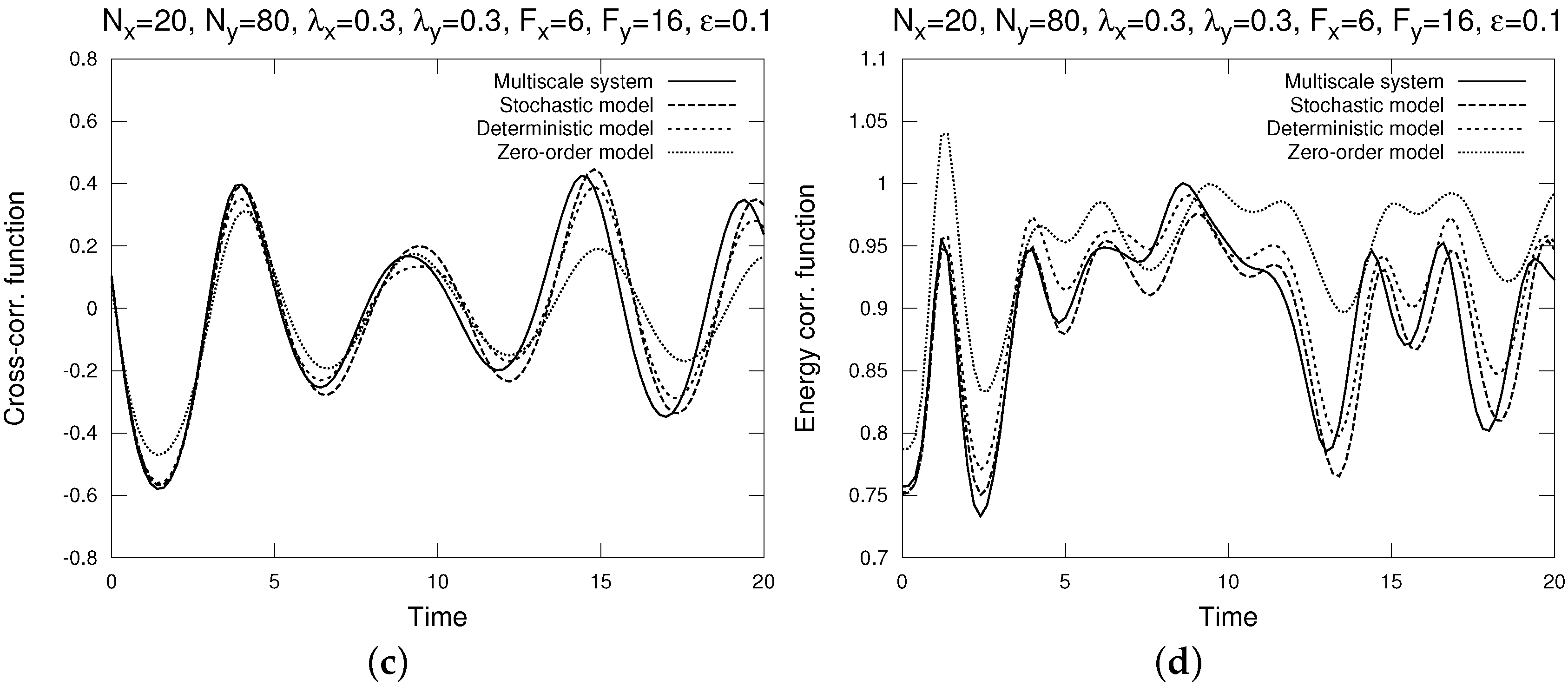
Here we present the comparison of different statistics for the dynamical regime with weak chaos and mixing at slow variables (achieved by setting ${\lambda }_x={\lambda }_y=0.35$) and weak time scale separation (achieved by setting $\epsilon =0.1$). In Figure 3 we show the distribution density functions, time auto-correlation functions, time cross-correlation functions, and energy auto-correlation functions for the multiscale dynamics in Equations (35a)–(35b), and three different kinds of the reduced models: the new stochastic reduced model, the deterministic reduced model from [35], and the zero-order reduced model with constant parameterization of coupling terms. Here we can see a significant improvement between the deterministic reduced model from [35] and the new stochastic reduced model. In particular, what apparently happens here is that the deterministic reduced model from [35] turns out to be less chaotic and mixing than the original multiscale dynamics at slow variables (observe that the distribution density is very spiky for the deterministic reduced model, while the time auto- and cross-correlation functions are less mixing, and the energy auto-correlation function is more sub-Gaussian than those for the multiscale dynamics). Then, the introduction of the stochastic term results in improvement of mixing and sub-Gaussianity, and also smoothes out the spikes on the distribution density, resulting in better approximation of the multiscale dynamics. Table 3 confirms that there is improvement of statistics error-wise with the introduction of the stochastic term in the new reduced model.

Table 3. Relative errors between the slow variables of the full multiscale system, and different reduced models, computed for the plots in Figure 3. $F_x=6$, $F_y=16$, ${\lambda }_x={\lambda }_y=0.35$, $\epsilon =0.1$.

Rel. Error	Stochastic	Deterministic	Zero-Order
Density	$2.166\times {10}^{-2}$	$4.83\times {10}^{-2}$	$7.516\times {10}^{-2}$
Corr.	$0.2322$	$0.2335$	$0.3584$
Cross-corr.	$0.2277$	$0.2346$	$0.3557$
Energy corr.	$2.858\times {10}^{-2}$	$5.031\times {10}^{-2}$	$0.2163$

Table 3. Relative errors between the slow variables of the full multiscale system, and different reduced models, computed for the plots in Figure 3. $F_x=6$, $F_y=16$, ${\lambda }_x={\lambda }_y=0.35$, $\epsilon =0.1$.

Rel. Error	Stochastic	Deterministic	Zero-Order
Density	$2.166\times {10}^{-2}$	$4.83\times {10}^{-2}$	$7.516\times {10}^{-2}$
Corr.	$0.2322$	$0.2335$	$0.3584$
Cross-corr.	$0.2277$	$0.2346$	$0.3557$
Energy corr.	$2.858\times {10}^{-2}$	$5.031\times {10}^{-2}$	$0.2163$

Figure 3. (a) Distribution density function; (b) time auto-correlation function; (c) time cross-correlation function; (d) energy auto-correlation function. $F_x=6$, $F_y=16$, ${\lambda }_x={\lambda }_y=0.35$, $\epsilon =0.1$.

Figure 3. (a) Distribution density function; (b) time auto-correlation function; (c) time cross-correlation function; (d) energy auto-correlation function. $F_x=6$, $F_y=16$, ${\lambda }_x={\lambda }_y=0.35$, $\epsilon =0.1$.

4.4. Weak Mixing at Slow Variables With Strong Time Scale Separation

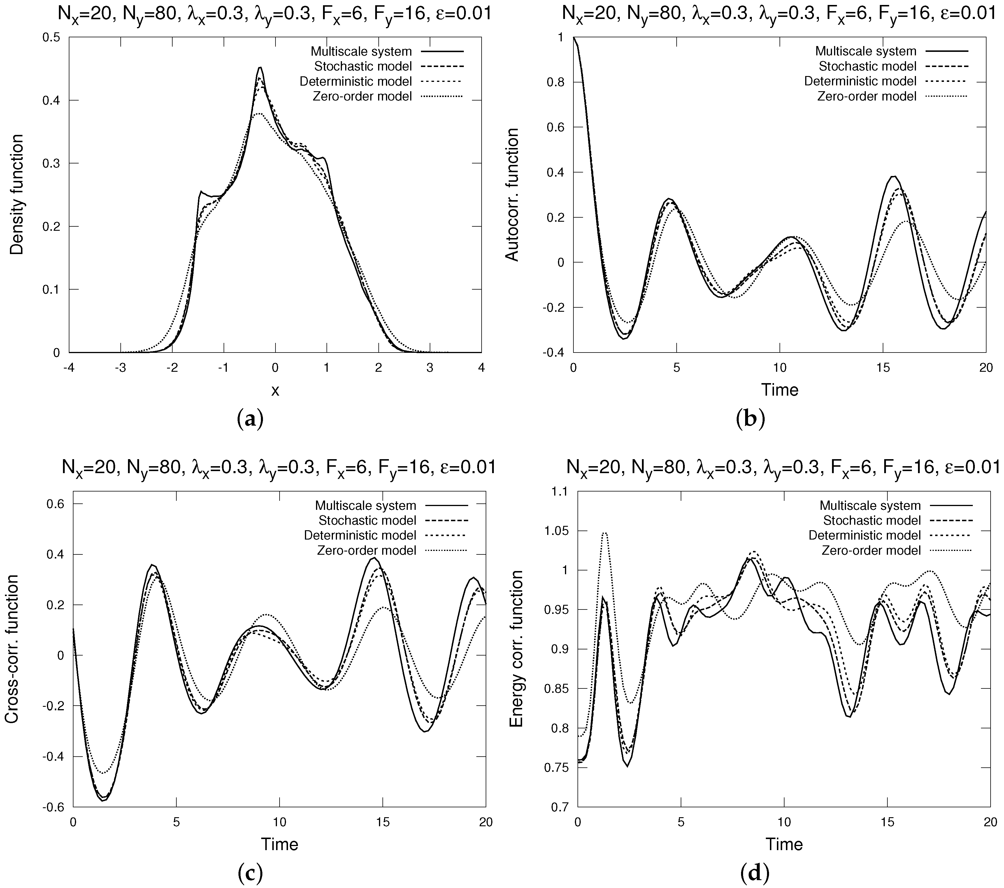
Here we present the comparison of different statistics for the dynamical regime with weak chaos and mixing at slow variables (achieved by setting ${\lambda }_x={\lambda }_y=0.35$) and strong time scale separation (achieved by setting $\epsilon =0.01$). In Figure 4 we show the distribution density functions, time auto-correlation functions, time cross-correlation functions, and energy auto-correlation functions for the multiscale dynamics in Equations (35a)–(35b), and three different kinds of the reduced models: the new stochastic reduced model, the deterministic reduced model from [35], and the zero-order reduced model with constant parameterization of coupling terms. Here, again, we can see a significant improvement between the deterministic reduced model from [35] and the new stochastic reduced model, however, in a somewhat reverse way if compared to the previous set-up with weak time scale separation. Here observe that the deterministic reduced model is more chaotic and mixing than the slow variables of the multiscale dynamics, and the stochastic term makes the new model less chaotic and mixing to better match the multiscale dynamics. While at first seeming counter-intuitive, this effect can happen due to the stochastic noise pushing the solution off the unstable manifold of the deterministic system (where the chaotic and mixing motion occurs) into the dissipative absorbing region surrounding the system’s attractor while not having enough strength to compensate for the lack of chaos and mixing with its own random forcing. In fact, the same (but somewhat weaker) effect can also be observed in Figure 1 and Figure 2 for weaker coupling and stronger chaos and mixing, so one can presume that it should be generally common in stochastic reduced models, especially if the time scale separation is strong and, because of that, the stochastic noise is weak enough to produce its own mixing. Table 4 confirms that there is some improvement of statistics error-wise with the introduction of the stochastic term in the new reduced model.

Table 4. Relative errors between the slow variables of the full multiscale system, and different reduced models, computed for the plots in Figure 4. $F_x=6$, $F_y=16$, ${\lambda }_x={\lambda }_y=0.35$, $\epsilon =0.01$.

Rel. Error	Stochastic	Deterministic	Zero-Order
Density	$6.237\times {10}^{-2}$	$7.716\times {10}^{-2}$	$0.1088$
Corr.	$0.2629$	$0.2752$	$0.3769$
Cross-corr.	$0.2556$	$0.2684$	$0.3726$
Energy corr.	$0.1254$	$0.1846$	$0.3059$

Table 4. Relative errors between the slow variables of the full multiscale system, and different reduced models, computed for the plots in Figure 4. $F_x=6$, $F_y=16$, ${\lambda }_x={\lambda }_y=0.35$, $\epsilon =0.01$.

Rel. Error	Stochastic	Deterministic	Zero-Order
Density	$6.237\times {10}^{-2}$	$7.716\times {10}^{-2}$	$0.1088$
Corr.	$0.2629$	$0.2752$	$0.3769$
Cross-corr.	$0.2556$	$0.2684$	$0.3726$
Energy corr.	$0.1254$	$0.1846$	$0.3059$

Figure 4. (a) Distribution density function; (b) time auto-correlation function; (c) time cross-correlation function; (d) energy auto-correlation function. $F_x=6$, $F_y=16$, ${\lambda }_x={\lambda }_y=0.35$, $\epsilon =0.01$.

Figure 4. (a) Distribution density function; (b) time auto-correlation function; (c) time cross-correlation function; (d) energy auto-correlation function. $F_x=6$, $F_y=16$, ${\lambda }_x={\lambda }_y=0.35$, $\epsilon =0.01$.

5. Conclusions

In the current work we improve the recently developed method [35,36] for deterministic reduced models of multiscale dynamics with the higher-order additive stochastic term which parameterizes the slow-fast interactions with random noise. The method is based on the homogenization techniques for multiscale systems [49] and offers a practical way of creating stochastic reduced models for a broad range of general multiscale processes. As demonstrated above in Section 3, the stochastic term upgrade comes at no additional computational cost for systems with linear coupling between slow and fast variables, as it uses the same time correlation matrix of the fast variables for a fixed state of the slow variables as the response term in the deterministic part of coupling parameterization. Another practical advantage of the new method is that it does not require an explicit time-scale separation parameter between the slow and fast variables of multiscale dynamics. We tested the new method numerically using the two-scale Lorenz 96 model with linear coupling between the slow and fast variables in a range of dynamical regimes with weak/strong time-scale separation, chaos and mixing at the slow variables. The new stochastic reduced model consistently improved the results of the previously developed deterministic approach [35,36] in the two different dynamical regimes:

• In the situation where the deterministic reduced model was less chaotic and weaker mixing than the slow variables of the full multiscale dynamics, the stochastic model was more chaotic and stronger mixing, due to stochastic forcing smoothing out spikes in distribution density and introducing random decorrelation in time auto- and cross-correlation functions.
• In the situation where the deterministic reduced model was more chaotic and stronger mixing than the slow variables of the full multiscale dynamics, the stochastic model suppressed chaos and mixing in the reduced dynamics. While this effect seems somewhat counter-intuitive, it can be explained by the stochastic noise pushing the solution off the unstable manifold of the deterministic system (where the chaotic and mixing motion occurs) into the dissipative region around the system’s attractor, while not having enough random force to increase chaos and mixing on its own.

In the future work, we plan to extend the new method of stochastic parameterization of reduced slow dynamics onto multiplicative stochastic forcing parameterization. Observe that the additive stochastic forcing parameterization in the current work emerges from the constant diffusion matrix approximation above in Section 3. However, if the constant diffusion matrix approximation is improved by including its higher order Taylor expansion terms (as was done to the deterministic coupling parameterization in [35,36]), the inclusion of the higher-order terms will result in the multiplicative coupling with the diffusion matrix of the reduced model being a function of the slow variables. For the multiplicative diffusion matrix approximation, we plan to use an approach similar to that in [35,36].

References

- Franzke, C.; Majda, A.; Vanden-Eijnden, E. Low-order stochastic model reduction for a realistic barotropic model climate. J. Atmos. Sci. 2005, 62, 1722–1745. [Google Scholar] [CrossRef]
- Hasselmann, K. Stochastic Climate Models: Part I. Theory. Tellus 1976, 28, 473–485. [Google Scholar] [CrossRef]
- Buizza, R.; Miller, M.; Palmer, T. Stochastic representation of model uncertainty in the ECMWF Ensemble Prediction System. Q. J. R. Meteor. Soc. 1999, 125, 2887–2908. [Google Scholar] [CrossRef]
- Palmer, T. A nonlinear dynamical perspective on model error: A proposal for nonlocal stochastic-dynamic parameterization in weather and climate prediction models. Q. J. R. Meteor. Soc. 2001, 127, 279–304. [Google Scholar] [CrossRef]
- Branstator, G.; Berner, J. Linear and nonlinear signatures in planetary wave dynamics of an AGCM: Phase space tendencies. J. Atmos. Sci. 2005, 62, 1792–1811. [Google Scholar] [CrossRef]
- Majda, A.; Franzke, C.; Crommelin, D. Normal forms for reduced stochastic climate models. Proc. Natl. Acad. Sci. USA 2009, 97, 12413–12417. [Google Scholar] [CrossRef] [PubMed]
- Kravtsov, S.; Kondrashov, D.; Ghil, M. Multilevel regression modeling of nonlinear processes: Derivation and applications to climatic variability. J. Clim. 2005, 18, 4404–4424. [Google Scholar] [CrossRef]
- Liu, D.; Vanden-Eijnden, E. Analysis of multiscale methods for stochastic differential equations. Commun. Pure Appl. Math. 2005, 58, 1544–1585. [Google Scholar]
- Fatkullin, I.; Vanden-Eijnden, E. A computational strategy for multiscale systems with applications to Lorenz 96 model. J. Comp. Phys. 2004, 200, 605–638. [Google Scholar] [CrossRef]
- Papanicolaou, G. Introduction to the Asymptotic Analysis of Stochastic Equations. Modern Modeling of Continuum Phenomena; Di Prima, R., Ed.; American Mathematical Society: Providence, RI, USA, 1977; Volume 16. [Google Scholar]
- Vanden-Eijnden, E. Numerical Techniques for multiscale dynamical systems with stochastic effects. Commun. Math. Sci. 2003, 1, 385–391. [Google Scholar] [CrossRef]
- Volosov, V. Averaging in systems of ordinary differential equations. Russ. Math. Surv. 1962, 17, 1–126. [Google Scholar] [CrossRef]
- Uhlenbeck, G.; Ornstein, L. On the theory of the Brownian motion. Phys. Rev. 1930, 36, 823–841. [Google Scholar] [CrossRef]
- Arnold, L.; Imkeller, P.; Wu, Y. Reduction of Deterministic Coupled Atmosphere-Ocean Models to Stochastic Ocean Models: A Numerical Case Study of the Lorenz-Maas System. Dyn. Syst. 2003, 18, 295–350. [Google Scholar] [CrossRef]
- Melbourne, I.; Stuart, A. A note on diffusion limits of chaotic skew product flows. Nonlinearity 2011, 24, 1361–1367. [Google Scholar] [CrossRef]
- Gottwald, G.; Melbourne, I. Homogenization for deterministic maps and multiplicative noise. Proc. R. Soc. 2013, A469, 20130201. [Google Scholar] [CrossRef]
- Kelly, D.; Melbourne, I. Deterministic Homogenization for Fast-Slow Systems with Chaotic Noise. Available online: http://xxx.lanl.gov/abs/1409.5748 (accessed on 18 December 2015).
- Kifer, Y. L2 Diffusion Approximation for Slow Motion in Averaging. Stoch. Dyn. 2003, 3, 213–246. [Google Scholar] [CrossRef]
- Crommelin, D.; Vanden-Eijnden, E. Subgrid scale parameterization with conditional Markov chains. J. Atmos. Sci. 2008, 65, 2661–2675. [Google Scholar] [CrossRef]
- Majda, A.; Timofeyev, I.; Vanden-Eijnden, E. Models for stochastic climate prediction. Proc. Natl. Acad. Sci. USA 1999, 96, 14687–14691. [Google Scholar] [CrossRef] [PubMed]
- Majda, A.; Timofeyev, I.; Vanden-Eijnden, E. Systematic strategies for stochastic mode reduction in climate. J. Atmos. Sci. 2003, 60, 1705–1722. [Google Scholar] [CrossRef]
- Majda, A.; Timofeyev, I.; Vanden-Eijnden, E. A Mathematical Framework for Stochastic Climate Models. Commun. Pure Appl. Math. 2001, 54, 891–974. [Google Scholar] [CrossRef]
- Majda, A.; Timofeyev, I.; Vanden-Eijnden, E. A priori Tests of a Stochastic Mode Reduction Strategy. Phys. D 2002, 170, 206–252. [Google Scholar] [CrossRef]
- Wilks, D. Effects of stochastic parameterizations in the Lorenz ’96 system. Q. J. R. Meteorol. Soc. 2005, 131, 389–407. [Google Scholar] [CrossRef]
- Katsoulakis, M.; Vlachos, G. Hierarchical kinetic Monte Carlo simulations for diffusion of interacting molecules. J. Chem. Phys. 2003, 112, 9412–9427. [Google Scholar] [CrossRef]
- Franzke, C.; Majda, A. Low-order stochastic mode reduction for a prototype atmospheric GCM. J. Atmos. Sci. 2006, 63, 457–479. [Google Scholar] [CrossRef]
- Branstator, G. Low-frequency patterns induced by stationary waves. J. Atmos. Sci. 1990, 47, 629–648. [Google Scholar] [CrossRef]
- Newman, M.; Sardeshmukh, P.; Penland, C. Stochastic forcing of the wintertime extratropical flow. J. Atmos. Sci. 1997, 54, 435–455. [Google Scholar] [CrossRef]
- Whitaker, J.; Sardeshmukh, P. A linear theory of extratropical synoptic eddy statistics. J. Atmos. Sci. 1998, 55, 237–258. [Google Scholar] [CrossRef]
- Zhang, Y.; Held, I. A linear stochastic model of a GCM’s midlatitude storm tracks. J. Atmos. Sci. 1999, 56, 3416–3435. [Google Scholar] [CrossRef]
- Majda, A.; Khouider, B. Stochastic and mesoscopic models for tropical convection. Proc. Natl. Acad. Sci. USA 2002, 99, 1123–1128. [Google Scholar] [CrossRef] [PubMed]
- Khouider, B.; Majda, A.; Katsoulakis, M. Coarse grained stochastic models for tropical convection. Proc. Natl. Acad. Sci. USA 2003, 100, 11941–11946. [Google Scholar] [CrossRef] [PubMed]
- Azencott, R.; Beri, A.; Timofeyev, I. Sub-sampling and Parametric Estimation for Multiscale Dynamics. Commun. Math. Sci. 2013, 11, 939–970. [Google Scholar] [CrossRef]
- Vannitsem, S. Stochastic Modelling and Predictability: Analysis of a Low-Order Coupled Ocean-Atmosphere Model. Phil. Trans. R. Soc. 2014, 372. [Google Scholar] [CrossRef] [PubMed]
- Abramov, R. A simple linear response closure approximation for slow dynamics of a multiscale system with linear coupling. Multiscale Model. Simul. 2012, 10, 28–47. [Google Scholar] [CrossRef]
- Abramov, R. A simple closure approximation for slow dynamics of a multiscale system: Nonlinear and multiplicative coupling. Multiscale Model. Simul. 2013, 11, 134–151. [Google Scholar] [CrossRef]
- Abramov, R. Short-time linear response with reduced-rank tangent map. Chin. Ann. Math. 2009, 30, 447–462. [Google Scholar] [CrossRef]
- Abramov, R. Approximate linear response for slow variables of deterministic or stochastic dynamics with time scale separation. J. Comput. Phys. 2010, 229, 7739–7746. [Google Scholar] [CrossRef]
- Abramov, R. Improved linear response for stochastically driven systems. Front. Math. China 2012, 7, 199–216. [Google Scholar] [CrossRef]
- Abramov, R.; Majda, A. New Approximations and Tests of Linear Fluctuation-Response for Chaotic Nonlinear Forced-Dissipative Dynamical Systems. J. Nonl. Sci. 2008, 18, 303–341. [Google Scholar] [CrossRef]
- Abramov, R.; Majda, A. Blended Response Algorithms for Linear Fluctuation-Dissipation for Complex Nonlinear Dynamical Systems. Nonlinearity 2007, 20, 2793–2821. [Google Scholar] [CrossRef]
- Abramov, R.; Majda, A. New algorithms for low frequency climate response. J. Atmos. Sci. 2009, 66, 286–309. [Google Scholar] [CrossRef]
- Majda, A.; Abramov, R.; Grote, M. Information Theory and Stochastics for Multiscale Nonlinear Systems. In CRM Monograph Series of Centre de Recherches Mathématiques, Université de Montréal; American Mathematical Society: Providence, RI, USA, 2005; Volume 25. [Google Scholar]
- Risken, H. The Fokker-Planck Equation, 2nd ed.; Springer-Verlag: New York, NY, USA, 1989. [Google Scholar]
- Lorenz, E. Predictability: A Problem Partly Solved. In Predictability of Weather and Climate; Palmer, T., Hagedom, R., Eds.; Cambridge University Press: England, UK, 1996. [Google Scholar]
- Lorenz, E.; Emanuel, K. Optimal Sites for Supplementary Weather Observations. J. Atmos. Sci. 1998, 55, 399–414. [Google Scholar] [CrossRef]
- Franzke, C. Dynamics of low-frequency variability: Barotropic mode. J. Atmos. Sci. 2002, 59, 2909–2897. [Google Scholar] [CrossRef]
- Selten, F. An efficient description of the dynamics of barotropic flow. J. Atmos. Sci. 1995, 52, 915–936. [Google Scholar] [CrossRef]
- Pavliotis, G.; Stuart, A. Multiscale Methods: Averaging and Homogenization; Springer: Berlin, Germany, 2008. [Google Scholar]
- Gikhman, I.; Skorokhod, A. Introduction to the Theory of Random Processes; Courier Dover Publications: Mineola, NY, USA, 1969. [Google Scholar]
- Abramov, R. Suppression of chaos at slow variables by rapidly mixing fast dynamics through linear energy-preserving coupling. Commun. Math. Sci. 2012, 10, 595–624. [Google Scholar] [CrossRef]
© 2015 by the authors; licensee MDPI, Basel, Switzerland. This article is an open access article distributed under the terms and conditions of the Creative Commons Attribution license ( http://creativecommons.org/licenses/by/4.0/).
Share and Cite
MDPI and ACS Style
Abramov, R. A Simple Stochastic Parameterization for Reduced Models of Multiscale Dynamics. Fluids 2016, 1, 2. https://doi.org/10.3390/fluids1010002
AMA Style
Abramov R. A Simple Stochastic Parameterization for Reduced Models of Multiscale Dynamics. Fluids. 2016; 1(1):2. https://doi.org/10.3390/fluids1010002
Chicago/Turabian StyleAbramov, Rafail. 2016. "A Simple Stochastic Parameterization for Reduced Models of Multiscale Dynamics" Fluids 1, no. 1: 2. https://doi.org/10.3390/fluids1010002