

Automatic Estimation of the Interference Subspace Dimension Threshold in the Subspace Projection Algorithms of Magnetoencephalography Based on Evoked State Data

Abstract
:1. Introduction
2. Materials and Methods
2.1. Subspace Projection Algorithm
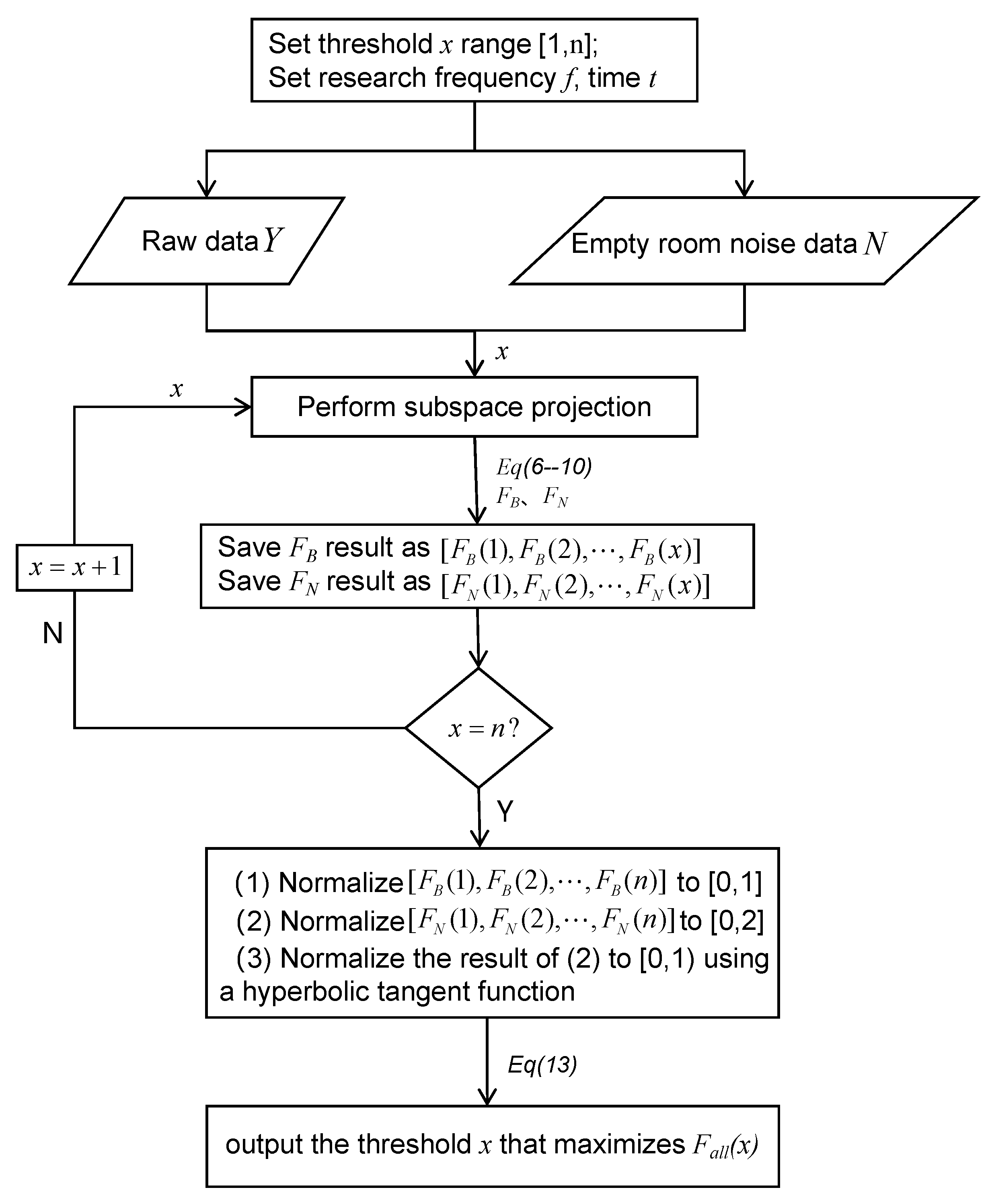
2.2. Threshold Estimation Algorithm
2.3. Experiments
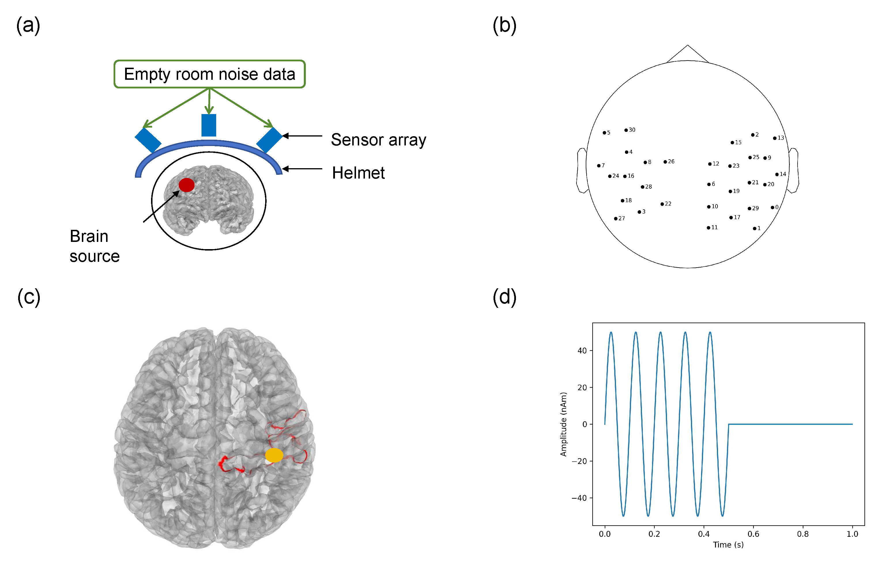
2.3.1. Simulation Experiment
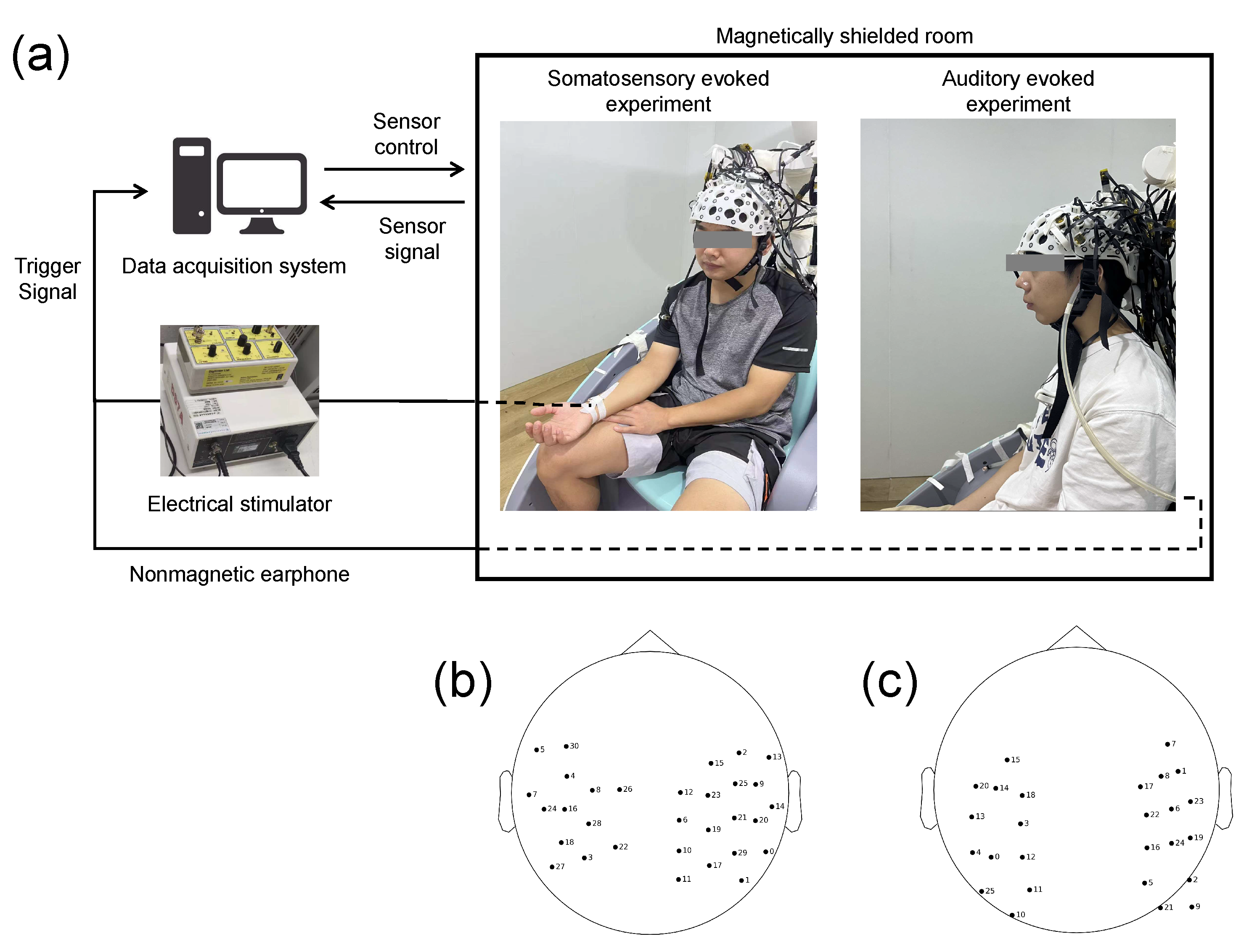
2.3.2. Stimulus-Evoked Experiments
2.3.3. Data Processing
2.3.4. Evaluation Metrics
3. Results
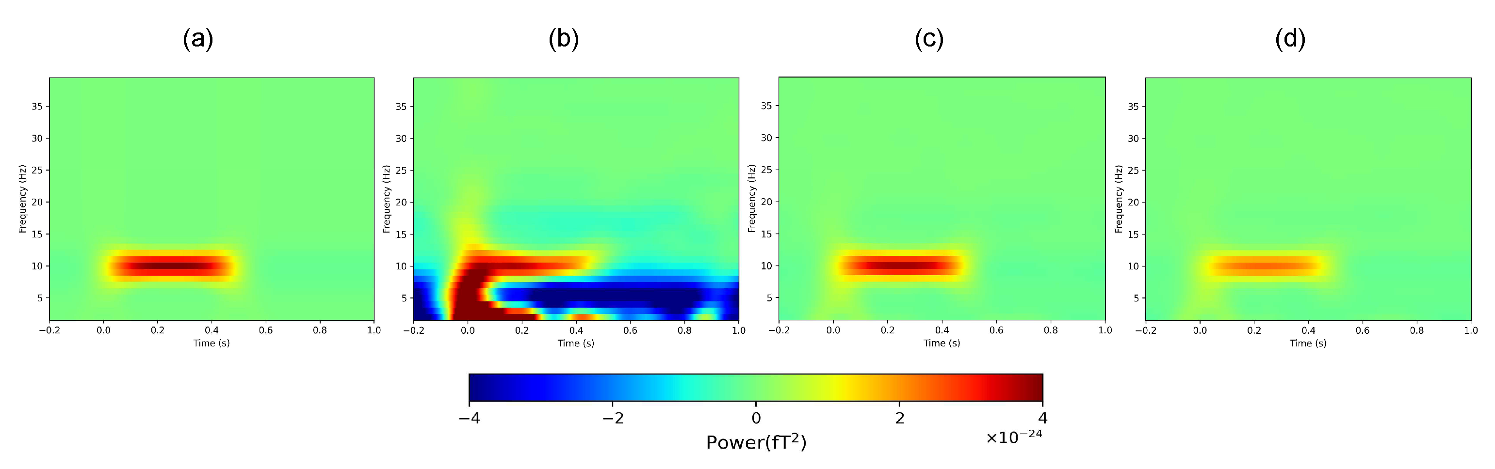
3.1. Simulation Experiment
3.2. Somatosensory-Evoked Experiment
3.3. Auditory-Evoked Experiment
4. Discussion
5. Conclusions
Author Contributions
Funding
Institutional Review Board Statement
Informed Consent Statement
Data Availability Statement
Conflicts of Interest
References
- Fred, A.L.; Kumar, S.N.; Kumar Haridhas, A.; Ghosh, S.; Purushothaman Bhuvana, H.; Sim, W.K.J.; Vimalan, V.; Givo, F.A.S.; Jousmäki, V.; Padmanabhan, P.; et al. A brief introduction to magnetoencephalography (MEG) and its clinical applications. Brain Sci. 2022, 12, 788. [Google Scholar] [CrossRef]
- Geller, A.S.; Teale, P.; Kronberg, E.; Ebersole, J.S. Magnetoencephalography for Epilepsy Presurgical Evaluation. Curr. Neurol. Neurosci. Rep. 2024, 24, 35–46. [Google Scholar] [CrossRef]
- Marco, E.J.; Khatibi, K.; Hill, S.S.; Siegel, B.; Arroyo, M.S.; Dowling, A.F.; Neuhaus, J.M.; Sherr, E.H.; Hinkley, L.N.; Nagarajan, S.S. Children with autism show reduced somatosensory response: An MEG study. Autism Res. 2012, 5, 340–351. [Google Scholar] [CrossRef]
- Boto, E.; Holmes, N.; Leggett, J.; Roberts, G.; Shah, V.; Meyer, S.S.; Muñoz, L.D.; Mullinger, K.J.; Tierney, T.M.; Bestmann, S.; et al. Moving magnetoencephalography towards real-world applications with a wearable system. Nature 2018, 555, 657–661. [Google Scholar] [CrossRef] [PubMed]
- Tierney, T.M.; Holmes, N.; Mellor, S.; López, J.D.; Roberts, G.; Hill, R.M.; Boto, E.; Leggett, J.; Shah, V.; Brookes, M.J.; et al. Optically pumped magnetometers: From quantum origins to multi-channel magnetoencephalography. NeuroImage 2019, 199, 598–608. [Google Scholar] [CrossRef] [PubMed]
- Gross, J. Magnetoencephalography in cognitive neuroscience: A primer. Neuron 2019, 104, 189–204. [Google Scholar] [CrossRef] [PubMed]
- Iivanainen, J.; Stenroos, M.; Parkkonen, L. Measuring MEG closer to the brain: Performance of on-scalp sensor arrays. NeuroImage 2017, 147, 542–553. [Google Scholar] [CrossRef]
- Brookes, M.J.; Leggett, J.; Rea, M.; Hill, R.M.; Holmes, N.; Boto, E.; Bowtell, R. Magnetoencephalography with optically pumped magnetometers (OPM-MEG): The next generation of functional neuroimaging. Trends Neurosci. 2022, 45, 621–634. [Google Scholar] [CrossRef] [PubMed]
- Bruña, R.; Vaghari, D.; Greve, A.; Cooper, E.; Mada, M.O.; Henson, R.N. Modified MRI anonymization (de-facing) for improved MEG coregistration. Bioengineering 2022, 9, 591. [Google Scholar] [CrossRef]
- Iivanainen, J.; Zetter, R.; Grön, M.; Hakkarainen, K.; Parkkonen, L. On-scalp MEG system utilizing an actively shielded array of optically-pumped magnetometers. Neuroimage 2019, 194, 244–258. [Google Scholar] [CrossRef]
- Holmes, N.; Tierney, T.M.; Leggett, J.; Boto, E.; Mellor, S.; Roberts, G.; Hill, R.M.; Shah, V.; Barnes, G.R.; Brookes, M.J.; et al. Balanced, bi-planar magnetic field and field gradient coils for field compensation in wearable magnetoencephalography. Sci. Rep. 2019, 9, 14196. [Google Scholar] [CrossRef]
- Burgess, R.C. Recognizing and correcting MEG artifacts. J. Clin. Neurophysiol. 2020, 37, 508–517. [Google Scholar] [CrossRef]
- Seymour, R.A.; Alexander, N.; Mellor, S.; O’Neill, G.C.; Tierney, T.M.; Barnes, G.R.; Maguire, E.A. Interference suppression techniques for OPM-based MEG: Opportunities and challenges. NeuroImage 2022, 247, 118834. [Google Scholar] [CrossRef]
- Hanna, J.; Kim, C.; Müller-Voggel, N. External noise removed from magnetoencephalographic signal using independent component analyses of reference channels. J. Neurosci. Methods 2020, 335, 108592. [Google Scholar] [CrossRef]
- Boto, E.; Meyer, S.S.; Shah, V.; Alem, O.; Knappe, S.; Kruger, P.; Fromhold, T.M.; Lim, M.; Glover, P.M.; Morris, P.G.; et al. A new generation of magnetoencephalography: Room temperature measurements using optically-pumped magnetometers. NeuroImage 2017, 149, 404–414. [Google Scholar] [CrossRef]
- Sekihara, K.; Nagarajan, S.S. Subspace-based interference removal methods for a multichannel biomagnetic sensor array. J. Neural Eng. 2017, 14, 051001. [Google Scholar] [CrossRef] [PubMed]
- Uusitalo, M.A.; Ilmoniemi, R.J. Signal-space projection method for separating MEG or EEG into components. Med. Biol. Eng. Comput. 1997, 35, 135–140. [Google Scholar] [CrossRef] [PubMed]
- Taulu, S.; Simola, J.; Kajola, M. Applications of the signal space separation method. IEEE Trans. Signal Process. 2005, 53, 3359–3372. [Google Scholar] [CrossRef]
- Watanabe, T.; Kawabata, Y.; Ukegawa, D.; Kawabata, S.; Adachi, Y.; Sekihara, K. Removal of stimulus-induced artifacts in functional spinal cord imaging. In Proceedings of the 2013 35th Annual International Conference of the IEEE Engineering in Medicine and Biology Society (EMBC), Osaka, Japan, 3–7 July 2013; pp. 3391–3394. [Google Scholar] [CrossRef]
- Taulu, S.; Simola, J. Spatiotemporal signal space separation method for rejecting nearby interference in MEG measurements. Phys. Med. Biol. 2006, 51, 1759. [Google Scholar] [CrossRef] [PubMed]
- Sekihara, K.; Kawabata, Y.; Ushio, S.; Sumiya, S.; Kawabata, S.; Adachi, Y.; Nagarajan, S.S. Dual signal subspace projection (DSSP): A novel algorithm for removing large interference in biomagnetic measurements. J. Neural Eng. 2016, 13, 036007. [Google Scholar] [CrossRef]
- Ramírez, R.R.; Kopell, B.H.; Butson, C.R.; Hiner, B.C.; Baillet, S. Spectral signal space projection algorithm for frequency domain MEG and EEG denoising, whitening, and source imaging. NeuroImage 2011, 56, 78–92. [Google Scholar] [CrossRef] [PubMed]
- Wang, R.; Wu, H.; Liang, X.; Cao, F.; Xiang, M.; Gao, Y.; Ning, X. Optimization of Signal Space Separation for Optically Pumped Magnetometer in Magnetoencephalography. Brain Topogr. 2023, 36, 350–370. [Google Scholar] [CrossRef]
- Holmes, N.; Bowtell, R.; Brookes, M.J.; Taulu, S. An Iterative Implementation of the Signal Space Separation Method for Magnetoencephalography Systems with Low Channel Counts. Sensors 2023, 23, 6537. [Google Scholar] [CrossRef]
- Medvedovsky, M.; Taulu, S.; Bikmullina, R.; Ahonen, A.; Paetau, R. Fine tuning the correlation limit of spatio-temporal signal space separation for magnetoencephalography. J. Neurosci. Methods 2009, 177, 203–211. [Google Scholar] [CrossRef] [PubMed]
- Vieira, D.A.; Travassos, L.; Saldanha, R.R.; Palade, V. Signal denoising in engineering problems through the minimum gradient method. Neurocomputing 2009, 72, 2270–2275. [Google Scholar] [CrossRef]
- Hu, L.; Xiao, P.; Zhang, Z.; Mouraux, A.; Iannetti, G.D. Single-trial time–frequency analysis of electrocortical signals: Baseline correction and beyond. Neuroimage 2014, 84, 876–887. [Google Scholar] [CrossRef] [PubMed]
- Schaefferkoetter, J.; Nai, Y.H.; Reilhac, A.; Townsend, D.W.; Eriksson, L.; Conti, M. Low dose positron emission tomography emulation from decimated high statistics: A clinical validation study. Med. Phys. 2019, 46, 2638–2645. [Google Scholar] [CrossRef] [PubMed]
- Marler, R.T.; Arora, J.S. Survey of multi-objective optimization methods for engineering. Struct. Multidiscip. Optim. 2004, 26, 369–395. [Google Scholar] [CrossRef]
- Yong, P.C.; Nordholm, S.; Dam, H.H. Optimization and evaluation of sigmoid function with a priori SNR estimate for real-time speech enhancement. Speech Commun. 2013, 55, 358–376. [Google Scholar] [CrossRef]
- An, N.; Cao, F.; Li, W.; Wang, W.; Xu, W.; Wang, C.; Gao, Y.; Xiang, M.; Ning, X. Multiple source detection based on spatial clustering and its applications on wearable OPM-MEG. IEEE Trans. Biomed. Eng. 2022, 69, 3131–3141. [Google Scholar] [CrossRef]
- Cao, F.; An, N.; Xu, W.; Wang, W.; Li, W.; Wang, C.; Yang, Y.; Xiang, M.; Gao, Y.; Ning, X. OMMR: Co-registration toolbox of OPM-MEG and MRI. Front. Neurosci. 2022, 16, 984036. [Google Scholar] [CrossRef]
- Del Gratta, C.; Della Penna, S.; Ferretti, A.; Franciotti, R.; Pizzella, V.; Tartaro, A.; Torquati, K.; Bonomo, L.; Romani, G.L.; Rossini, P.M. Topographic organization of the human primary and secondary somatosensory cortices: Comparison of fMRI and MEG findings. Neuroimage 2002, 17, 1373–1383. [Google Scholar] [CrossRef]
- Gramfort, A.; Luessi, M.; Larson, E.; Engemann, D.A.; Strohmeier, D.; Brodbeck, C.; Goj, R.; Jas, M.; Brooks, T.; Parkkonen, L.; et al. MEG and EEG data analysis with MNE-Python. Front. Neurosci. 2013, 7, 267. [Google Scholar] [CrossRef]
- An, N.; Cao, F.; Li, W.; Wang, W.; Xu, W.; Wang, C.; Xiang, M.; Gao, Y.; Sui, B.; Liang, A.; et al. Imaging somatosensory cortex responses measured by OPM-MEG: Variational free energy-based spatial smoothing estimation approach. Iscience 2022, 25, 103752. [Google Scholar] [CrossRef]
- Cheng, C.H.; Liu, C.Y.; Hsu, S.C.; Tseng, Y.J. Reduced coupling of somatosensory gating and gamma oscillation in panic disorder. Psychiatry Res. Neuroimaging 2021, 307, 111227. [Google Scholar] [CrossRef]
- Falet, J.P.R.; Côté, J.; Tarka, V.; Martínez-Moreno, Z.E.; Voss, P.; de Villers-Sidani, E. Mapping the human auditory cortex using spectrotemporal receptive fields generated with magnetoencephalography. Neuroimage 2021, 238, 118222. [Google Scholar] [CrossRef]
- Hämäläinen, M.; Hari, R.; Ilmoniemi, R.J.; Knuutila, J.; Lounasmaa, O.V. Magnetoencephalography-theory, instrumentation, and applications to noninvasive studies of the working human brain. Rev. Mod. Phys. 1993, 65, 413. [Google Scholar] [CrossRef]
- Hämäläinen, M.S.; Ilmoniemi, R.J. Interpreting magnetic fields of the brain: Minimum norm estimates. Med. Biol. Eng. Comput. 1994, 32, 35–42. [Google Scholar] [CrossRef]
- Tierney, T.M.; Alexander, N.; Mellor, S.; Holmes, N.; Seymour, R.; O’Neill, G.C.; Maguire, E.A.; Barnes, G.R. Modelling optically pumped magnetometer interference in MEG as a spatially homogeneous magnetic field. NeuroImage 2021, 244, 118484. [Google Scholar] [CrossRef]
- Helle, L.; Nenonen, J.; Larson, E.; Simola, J.; Parkkonen, L.; Taulu, S. Extended signal-space separation method for improved interference suppression in MEG. IEEE Trans. Biomed. Eng. 2020, 68, 2211–2221. [Google Scholar] [CrossRef]
- Zhao, R.; Wang, R.; Gao, Y.; Ning, X. Spatiotemporal extended homogeneous field correction method for reducing complex interference in OPM-MEG. Biomed. Signal Process. Control 2024, 94, 106236. [Google Scholar] [CrossRef]


| Method | Threshold | PE (fT) | MAE (fT) | LE (mm) | |
|---|---|---|---|---|---|
| SSP | x = 4 | 1.369 | 137.03 | 47.25 | 2.80 |
| x = 5 | 1.365 | 138.54 | 49.56 | 3.57 | |
| x = 3 | 1.295 | 149.75 | 51.25 | 3.32 | |
| x = 6 | 1.264 | 155.05 | 52.11 | 4.93 | |
| x = 7 | 1.175 | 159.04 | 54.77 | 5.48 | |
| S3P | x = 4 | 1.403 | 152.15 | 55.11 | 2.93 |
| x = 3 | 1.380 | 177.29 | 56.00 | 4.47 | |
| x = 5 | 1.363 | 188.26 | 59.29 | 3.05 | |
| x = 2 | 1.337 | 212.77 | 59.20 | 5.15 | |
| x = 6 | 1.302 | 201.89 | 59.71 | 5.57 |
Disclaimer/Publisher’s Note: The statements, opinions and data contained in all publications are solely those of the individual author(s) and contributor(s) and not of MDPI and/or the editor(s). MDPI and/or the editor(s) disclaim responsibility for any injury to people or property resulting from any ideas, methods, instructions or products referred to in the content. |
© 2024 by the authors. Licensee MDPI, Basel, Switzerland. This article is an open access article distributed under the terms and conditions of the Creative Commons Attribution (CC BY) license (https://creativecommons.org/licenses/by/4.0/).
Share and Cite
Zhao, R.; Wang, R.; Gao, Y.; Ning, X. Automatic Estimation of the Interference Subspace Dimension Threshold in the Subspace Projection Algorithms of Magnetoencephalography Based on Evoked State Data. Bioengineering 2024, 11, 428. https://doi.org/10.3390/bioengineering11050428
Zhao R, Wang R, Gao Y, Ning X. Automatic Estimation of the Interference Subspace Dimension Threshold in the Subspace Projection Algorithms of Magnetoencephalography Based on Evoked State Data. Bioengineering. 2024; 11(5):428. https://doi.org/10.3390/bioengineering11050428
Chicago/Turabian StyleZhao, Ruochen, Ruonan Wang, Yang Gao, and Xiaolin Ning. 2024. "Automatic Estimation of the Interference Subspace Dimension Threshold in the Subspace Projection Algorithms of Magnetoencephalography Based on Evoked State Data" Bioengineering 11, no. 5: 428. https://doi.org/10.3390/bioengineering11050428