1. Introduction
Ventricular assist devices (VADs) are mechanical systems aimed at supporting the blood circulation in patients with severe heart failure. After five decades of intensive development, various devices have become increasingly applied, typically as a “bridge to transplantation”,
i.e., for patients with no other alternative left [
1]. In addition, by assisting and, thus, unloading the failing cardiac ventricle, VADs have also been shown to contribute to some degree to myocardial recovery [
2,
3]. Currently, second and third generation VADs are poised to replace the first generation volume displacement VADs. They have been found to be superior in terms of survival rate and reduced adverse events [
4].
Feedback control strategies to physiologically adapt the operation of turbo dynamic VADs (tVADs) to the oxygen demand and to optimize left-ventricular unloading have been subject to continuous research [
5,
6,
7,
8,
9,
10]. A number of approaches for realizing a speed modulation of tVADs has been analyzed earlier. A square-wave speed profile was applied by Bearnson
et al. [
11] and Bourque
et al. [
12] to increase arterial pulse pressure, where the speed profile was not synchronized to the cardiac cycle. Different types of speed profiles, synchronized to the natural cardiac cycle, have been applied
in silico and
in vitro to analyze their influence on perfusion, pulse pressure and ventricular unloading [
13,
14,
15,
16,
17,
18].
In vivo experiments have been conducted to validate this approach [
19,
20]. Common among all previous research on this topic was the preselection of a certain speed profile, such as a sine wave or a square wave. In these studies, the parameters of the selected profile were varied to analyze the effect on relevant physiological quantities. Naturally, the outcome depended on the preselected speed profile.
We present a methodology that circumvents the limitation of preselecting a certain speed profile by the application of model-based numerical optimization. A physiologically motivated objective function was constructed, and the speed profile that minimizes this objective function was found by solving an optimal-control problem (OCP). By defining an OCP, no assumptions about the speed profile needed to be made in advance. Instead, the tVAD is expected to optimally interact with the circulatory system. Due to this absence of restrictions, we hypothesize that the optimized speed trajectory performs better than strategies with either a constant speed or predefined speed profiles.
Optimal control was applied to VADs in previous work. The flow field in a pulsatile volume-displacement VAD was optimized in order to reduce hemolysis and thrombus formation in the device in [
21]. In two other studies [
22,
23], the power consumption of a pusher plate-type VAD was minimized using the optimal control of a linear and time-invariant model of the VAD and a part of the systemic circulation. The methodology described in the current paper differs from previous work as follows: the cardiovascular system, including the beating heart, was entirely integrated in the optimization procedure. Considering this coupled system as a whole entity allowed for the optimization of the interaction between the VAD and the circulation system, rather than of just the performance of the isolated VAD.
In the current paper, a state-space model of the human circulation [
24] was used in connection with a mathematical model of a turbo dynamic blood pump. This full model was used for simulations with a constant pump speed, as well as with various sinusoidal speed profiles. A reduced version of the model was used to formulate the OCP, which was solved numerically. The validation of the optimized speed profiles on a hybrid mock circulation [
25] indicated that they can potentially be evaluated in a real blood pump.
2. Methods
In this section, three different methods for obtaining a pump speed profile are presented. Either a constant speed, a sinusoidal speed profile synchronized to the cardiac cycle or a speed profile obtained from the numerical solution of an OCP was applied. The first two cases are detailed in
Section 2.1, and the formulation, as well as the numerical solution procedure of the OCP are described in
Section 2.2. The solutions resulting from these methods were compared using a physiologically motivated objective function in
Section 3. For the first two methods, this objective function must be evaluated
a posteriori, because the speed profile was predefined and an exhaustive parameter sweep was performed. In the third method, the objective function is a part of the OCP, and its value, as well as the corresponding speed profile result from the solution of this OCP. To ensure a fair comparison of the various pump-actuation strategies, one additional parameter was fixed, namely the total cardiac output. This parameter represents the total amount of blood pumped to the circulatory system by both the heart and the blood pump. The reason for fixing the total cardiac output is outlined in the following.
The autoregulatory mechanisms ensure that the supply of oxygenated blood to the body conforms to its current needs. In order to allow for a fair comparison between any two speed profiles, the total cardiac output has to be equal for both. In the lumped-parameter models used in the current study, there is a unique relation between the activity of the baroreflex mechanisms, defining the arterial resistance, and the mean arterial pressure. These two quantities, namely the arterial resistance and mean pressure, define the total cardiac output. It is therefore sufficient to prescribe the cardiac output to ensure the comparability of different solutions. A value of
was imposed, which represents a physiologically plausible value for an adult person at rest [
26]. In the model used, this value implied a mean systemic arterial pressure of
. The results presented could also be reproduced for other perfusion levels. The fixation of the total cardiac output to
is also justified by the fact that the current study did not investigate the effect of the VAD actuation on the perfusion, but was focused on the heart-VAD interaction.
The model of the cardiovascular system used here was originally published in [
24]. An implementation in MATLAB/S
imulink® (The Mathworks Inc., Natick, MA, USA) of this model was used earlier [
25]. The pathologic case defined in [
24] was used for all investigations. It is defined by a raised heart rate of
and a reduced ventricular contractility.
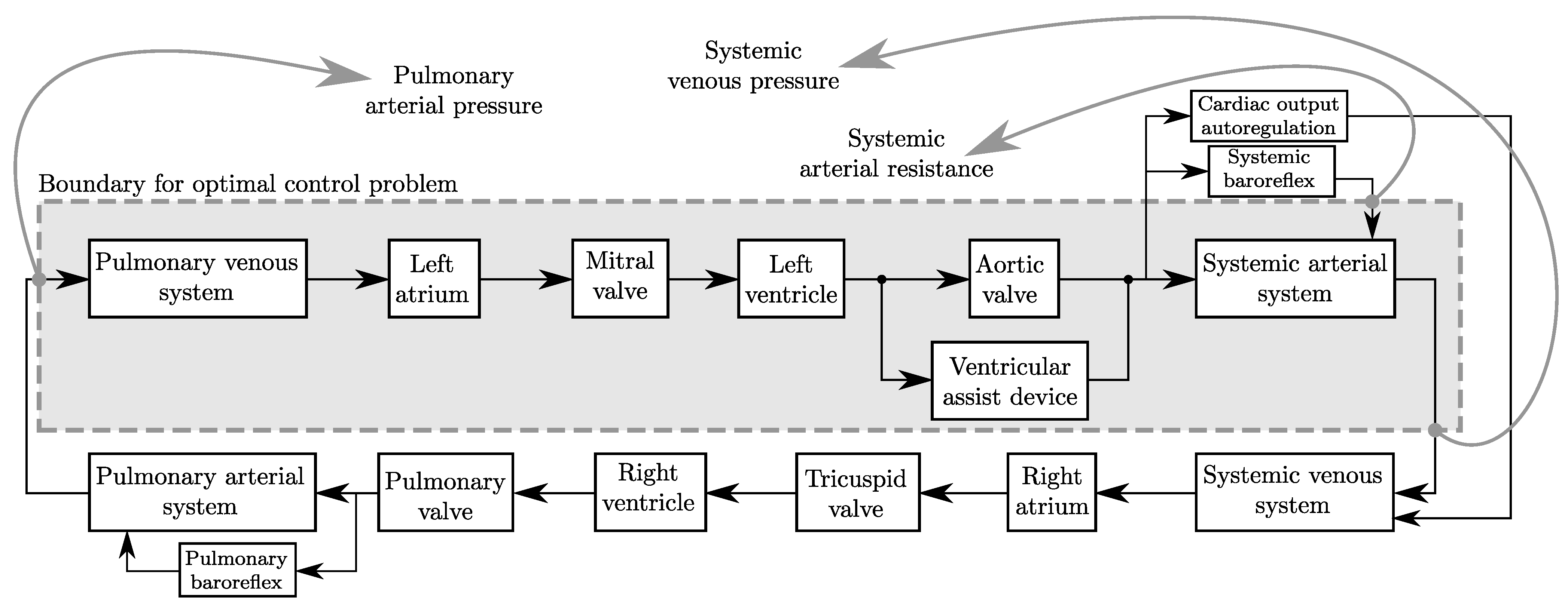
Figure 1 illustrates the structure of the model. The full model comprises the left and right atria and ventricles, the four heart valves and the systemic and the pulmonary circulation, each with an arterial and a venous section. The four contracting chambers of the heart are modeled based on the principle of time-varying elastance, which is the inverse of the compliance or the stiffness of the heart muscle wall. This stiffness varies during the cardiac cycle, thereby causing a contraction. The time-varying elastance is modeled by specific, empirically-derived curves that are described in the literature [
27]. Three independent autoregulatory mechanisms were modeled: the first mechanism adapts the flow resistance in the systemic arterial system based on the mean systemic arterial pressure; the second mechanism adapts the flow resistance in the pulmonary arterial system based on the mean pulmonary arterial pressure. Finally, the unstressed volume in the systemic veins is adapted based on the total cardiac output,
i.e., the venous tone is adapted. The simulated inflow cannula of the tVAD was connected with the left ventricle, and the simulated outflow cannula was attached to the aorta. This model was used to generate the constant speed and the sinusoidal speed profile solutions by forward simulation, as described in
Section 2.1.
Figure 1.
The subsystems of the numerical circulation model described in [
24,
25], including a ventricular assist device. The optimal-control problem (OCP) considered in the current paper is based on the reduced model indicated by the gray box. There are three boundary conditions that were computed by the full model: the pulmonary arterial pressure, the systemic venous pressure and the systemic arterial resistance. The latter is influenced by the baroreflex mechanism. These quantities do not change, as long as the total cardiac output and, thus, the mean arterial pressure are unchanged.
In order to reduce the size and the complexity of the OCP described in
Section 2.2, a reduced version of the model was used, as indicated by the gray box in
Figure 1. Different choices for the boundaries of the reduced model are possible. Since the cardiac output was fixed and only the left ventricle was supported, the influence of the pump control strategy on the right ventricle was negligible. The boundaries need to be chosen, such that the pump speed profile does not have an effect on the pressure waveform at the boundaries. Choosing the pulmonary arterial pressure and the systemic venous pressure has been shown to fulfill these requirements. For these boundary conditions, the trajectories resulting from the constant speed solution were applied. Furthermore, the systemic arterial resistance from the same solution was enforced during the optimization. This setup ensured that the demanded cardiac output of
led to the same mean systemic arterial pressure of
, as in the solutions obtained from the full model.
2.1. Simulation of the Reference Solutions
The solutions for the constant speed and the sinusoidal speed profile cases were generated by forward simulations of the full model. Thereby, the mean pump speed, , was regulated automatically, to yield the desired cardiac output of . In the constant speed case, there is one unique pump speed of that provides the desired cardiac output.
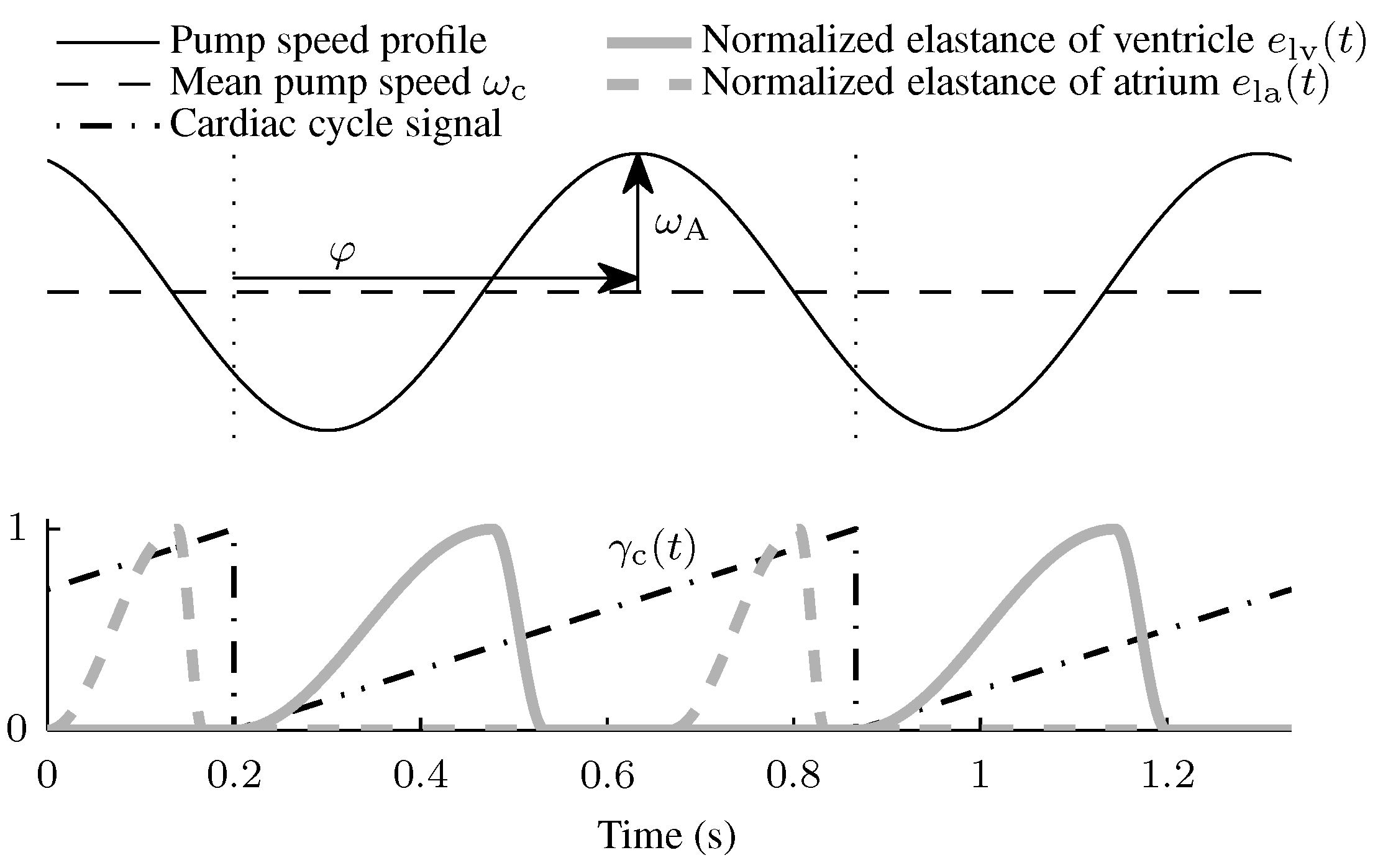
The sinusoidal speed profiles are illustrated in
Figure 2. They are defined as:
where
is the amplitude in
and
φ is the phase shift as a fraction of the duration of one cardiac cycle. The variable,
, is a periodic, sawtooth-shaped signal representing the progress through each cardiac cycle. The variables,
φ and
, range from 0 to 1, where
represents the onset of the ventricular systole. The phase offset of
was chosen, such that at a phase shift of
, the maximum tVAD speed occurs exactly at the onset of the ventricular systole.
Figure 2.
Timing of the sinusoidal speed profile with respect to the cardiac cycle. The start of a cardiac cycle was defined as the onset of the ventricular systole (dotted vertical lines). At these instants, the cardiac cycle signal, , which was used to generate the sinusoidal speed profile, is reset. For the sinusoidal speed profiles, the two parameters, φ (phase shift) and (amplitude), are defined.
A “brute-force” analysis was performed: The two parameters,
and
φ, were varied in small steps throughout their admissible range, and for each combination, a forward simulation was executed. The steps chosen were
and
. The data of the resulting 280 simulations were stored and can be used to evaluate any objective function, e.g., the one described by Equation (
6a) below.
2.2. Optimal-Control Problem
This section is divided into four parts.
Section 2.2.1 details the mathematical model of the reduced cardiovascular system.
Section 2.2.2 defines the mathematical model of the blood pump, and
Section 2.2.3 describes the formulation of the continuous-time OCP. Finally,
Section 2.2.4 describes the transformation of this OCP into a nonlinear program (NLP), as well as the method for solving it.
2.2.1. Reduced Model of the Cardiovascular System
The differential equations describing the cardiovascular system are:
where each state variable describes either a volume or a volume flow in the cardiovascular system; see
Table A1 in the
Appendix. The right-hand sides of most of these differential equations depend on pressures in the cardiovascular system that are static functions of the state variables. The pressures in the pulmonary vein and in the systemic arteries are calculated assuming constant compliance and a volume offset:
For the aortic pressure, visco-elasticity is taken into account, as well:
The pressures in the left atrium and the left ventricle are calculated using empirical time-varying elastance laws. For the left ventricle, a visco-elastic effect was included. Thus, the equations read:
The pressure-volume relations of the contracting chambers (left ventricle and left atrium) are defined as:
where the index,
i, represents either the left atrium or the left ventricle. Accordingly,
represents either the left atrial volume,
, or the left ventricular volume,
. The subscript,
, in Equation (
2n) denotes that the equation describes the passive pressure-volume relationship (relaxed muscle); the subscript,
, in Equation (
2o) denotes the active pressure-volume relationship (contracting muscle).
The model depends on several time-varying parameters: the pressures at the boundaries,
and
, the normalized elastance functions,
and
, and the internal resistance of the left ventricle,
.
Figure 2 shows the two normalized elastance functions:
The index,
i, denotes either the left ventricle (lv) or the left atrium (la). In the former case, the parameter,
, is equal to 0, and in the latter case the value of
accounts for the time delay between the contraction of the two chambers.
Table A2 in the
Appendix shows the parameter values used in Equation (2).
The slack variables,
and
, were used to model the heart valves, which impose a strictly non-negative flow. To achieve this non-smooth behavior, the following set of constraints needs to be satisfied [
28]:
2.2.2. Model of the Blood Pump
Two differential equations were used to describe the acceleration of the fluid in a mixed-flow blood pump (Deltastream DP2, Medos Medizintechnik AG, Stolberg, Germany) and the acceleration of the rotor shaft:
Here,
is the flow rate through the pump and
is the rotational speed of the pump. The variable,
, is the pump current. The “pressure head”,
H, and the “hydraulic torque”,
T, of the pump were stored in two-dimensional maps obtained from static measurements on the hybrid mock circulation. The parameter,
, relates the produced torque to the electric current and was supplied by the motor manufacturer. The fluid inertance,
, and the rotor inertia,
, were identified using dynamic measurements. The variables describing the pump model are summarized in
Table A3 in the
Appendix.
2.2.3. Formulation of the Optimal-Control Problem
The reduced model has
state variables. The first eight (
) describe the circulation Equation (2), whereas the two remaining ones (
) describe the mixed-flow blood pump Equation (4). The model has one control input, namely the pump current,
. The two slack variables,
and
, represent, from a structural point of view, two additional inputs. The control input and these two slack variables were gathered in the input vector,
, which, consequently, has the dimension
. All state variables were gathered in the state vector,
. The corresponding right-hand sides of the differential equations describing the model were stacked in the vector-valued “model function”,
f:
The mathematical representation of the optimization problem to be solved comprises an objective function Equation (
6a) and several constraints Equations (
6b)–(
6i):
The function,
L, in Equation (
6a) is an arbitrary function of the state variables and is described below. The time instances,
and
, denote the start of two consecutive cardiac cycles, where the heart rate is equal to
,
i.e.,
. The vector-valued continuity constraint Equation (
6b) ensures that, for a solution of the OCP, the model equations are satisfied. The constraint Equation (
6c) represents Equations (
3a) and (
3b), which model the heart valves. The constraint Equation (
6d) ensures the desired cardiac output of
,
A periodic solution was sought, defined by the constraints Equations (
6e) and (
6f). The constraints Equations (
6g) and (
6h) implement the upper and lower bounds on the state variables and the inputs, as specified in
Table A1 in the
Appendix. Different values were chosen for the lower bound on the pump flow,
. The standard value of 0 implies that no backflow occurs from the aorta to the left ventricle. The influence on the solution when a strictly positive flow was enforced is analyzed in
Section 3.4.
The objective function Equation (
6a) was chosen in accordance with physiological considerations. The application of a VAD can lead to a permanent closure of the aortic valve. Fusion of the aortic valvular cusps and a thrombus formation at the aortic valve may occur in this case [
29,
30,
31]. Including the flow through the aortic valve as the first component of the objective function allows solutions to be enforced where the flow through the aortic valve is maximized and, thus, opening of the valve is ensured. A further goal of the installation of a VAD is the unloading of the heart. Thus, a reduction of the hydraulic work the left ventricle needs to deliver was chosen as a second component of the objective function. The main task of a VAD is to maintain the perfusion of the patient, which was enforced by the perfusion constraint Equation (
6d).
The tradeoff between the two conflicting components of the objective function is adjusted by the weighting parameter,
. The objective function thus reads:
The parameter normalizes , such that the typical values of both components of the objective function are within the same numerical range. The parameter =133.3 × converts the units of from to J.
2.2.4. Numerical Solution of the Optimal-Control Problem
Direct transcription was applied to solve the OCP Equation (6), transforming the continuous-time problem into an NLP [
32,
33]. Despite its large size, the resulting NLP can be solved efficiently, due to its structure and the performance of current NLP solvers. Furthermore, this approach provides a straightforward handling of any type of constraints [
34].
The family of Radau collocation schemes was applied in this work [
35]. Collocation methods represent each state variable
as a polynomial and, thus, provide a continuous solution. When used in the context of direct transcription, their implicit nature is irrelevant. “Radau IIA” methods were chosen because to their advantageous stability properties [
36]. For the problem at hand, using a low-order method with a fine time discretization yielded the best results concerning the convergence of the NLP solver and the avoidance of local minima. In fact, the results shown below were obtained using the first-order representative of this collocation family, which is the well-known Euler-backward scheme.
All of the equations forming the OCP Equation (6) have to be discretized consistently. A grid of
N points was used, yielding
intervals of length
. The notation
was adopted. The continuity constraint Equation (
6b) was transformed to discrete defect constraints; all integrals became weighted sums, and the constraints on the inputs and on the state variables were imposed at the discretization points. Therefore, the continuous OCP Equation (6) is transformed to:
Equation (9) defines an NLP in
variables, namely
and
for
, which has
equality constraints. Its objective function Equation (
9a) is nonlinear in the NLP variables, and it has nonlinear constraints Equations (
9b) and (
9c), linear constraints Equations (
9d), (
9e) and (
9f), as well as simple bounds Equations (
9g) and (
9h). All state variables and inputs were scaled, such that the range between the lower and the upper bounds was mapped to the interval,
. This normalization ensures a similar magnitude of all NLP variables. The resulting improvement in numerical condition of the problem increased the reliability and the convergence speed of the NLP solver.
The equality-constrained NLP is commonly solved using a Newton-type iteration. Due to the required factorizations (or re-factorizations, respectively) of the large matrices involved, a typical runtime between
and
results [
37]. The second-order derivatives were approximated by an iterative update using first-order derivative information. Two factors are thus key for a fast solution of the OCP: (a) the reduction of the problem size and (b) the exploitation of the problem structure to reduce the number of evaluations of the objective and model functions. The following paragraphs outline the procedure to achieve both.
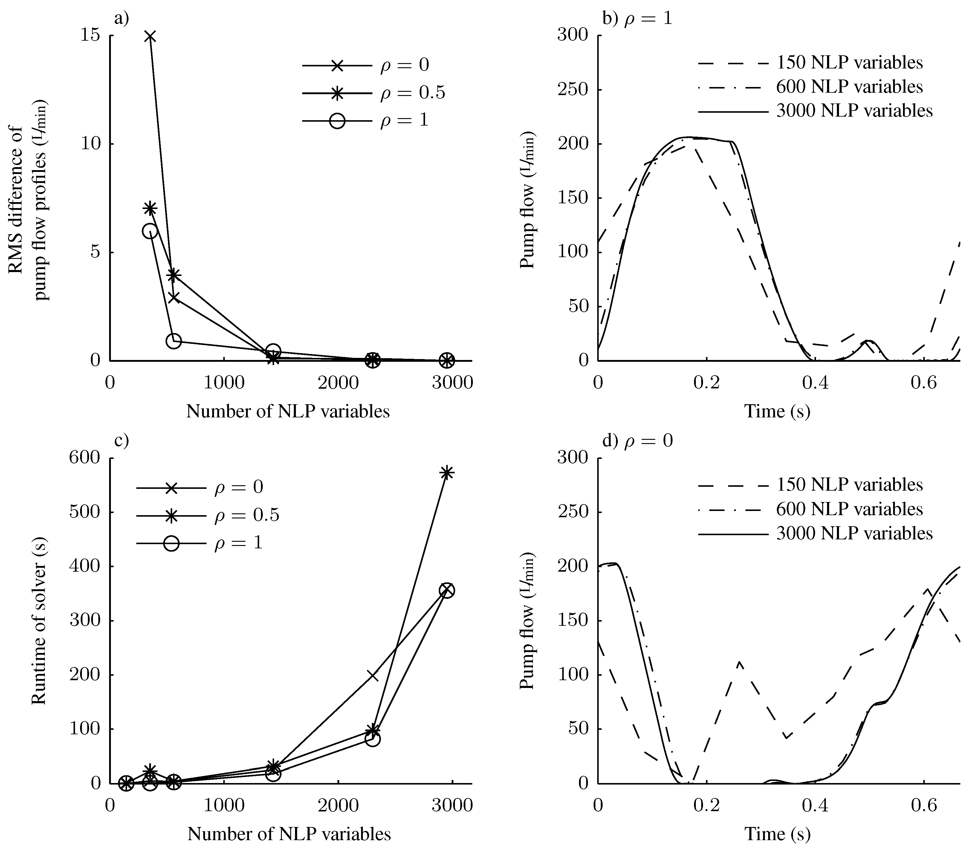
The problem size was kept small by first using a discretization with a constant step size of , resulting in discretization points. The resulting solution was then used to initialize a refined version of the problem. Namely, the step size was halved, which results in an NLP that is twice as large. However, since a close initial guess is available, only a few iterations are required to solve this NLP to the demanded tolerance. For all solutions presented below, two refinements were performed, which yielded a final step size of .
The Jacobian matrix contains the partial derivatives of the objective function Equation (
9a) and of all constraints Equations (
9b)–(
9f) with respect to the NLP variables. Since the objective function and each constraint depend on a few NLP variables only, most of its entries are zero. This fact is termed “sparsity”, and its exploitation is the key to an efficient numerical solution of directly transcribed OCPs [
38]. Most importantly, the objective function,
L, and the model function,
f, only occur in Equations (
9a) and (
9b), respectively. Furthermore, their arguments are the state variables and the inputs at the same discretization point. Therefore, all derivative information required for the construction of the Jacobian matrix is provided by the partial derivatives of the model function and of the objective function with respect to the state variables, as well as the inputs at each discretization node.
Any NLP solver can calculate the Jacobian matrix by numerical differentiation. However, depending on its algorithmic implementation, it is unable to fully exploit the problem sparsity. In order to always obtain the least possible number of evaluations of the objective and the model functions, the Jacobian matrix was constructed by custom code and was then passed to the NLP solver. Linear terms Equations (
9d)–(
9f) have constant derivatives, whereas simple bounds Equations (
9g)–(
9h) are handled directly by the NLP solver. The derivatives of objective function Equation (
9a) and of defect constraints Equation (
9b) were constructed from the derivatives of the objective and the model functions, which were calculated analytically.
As an NLP solver, SNOPT was used [
39]. Iteratively refining the problem discretization and providing the Jacobian matrix to the solver reduced the typical runtime for solving one OCP from about
to less than
. This reduction in computational time enabled large-scale parametric studies and a quick comparison of various problem formulations.
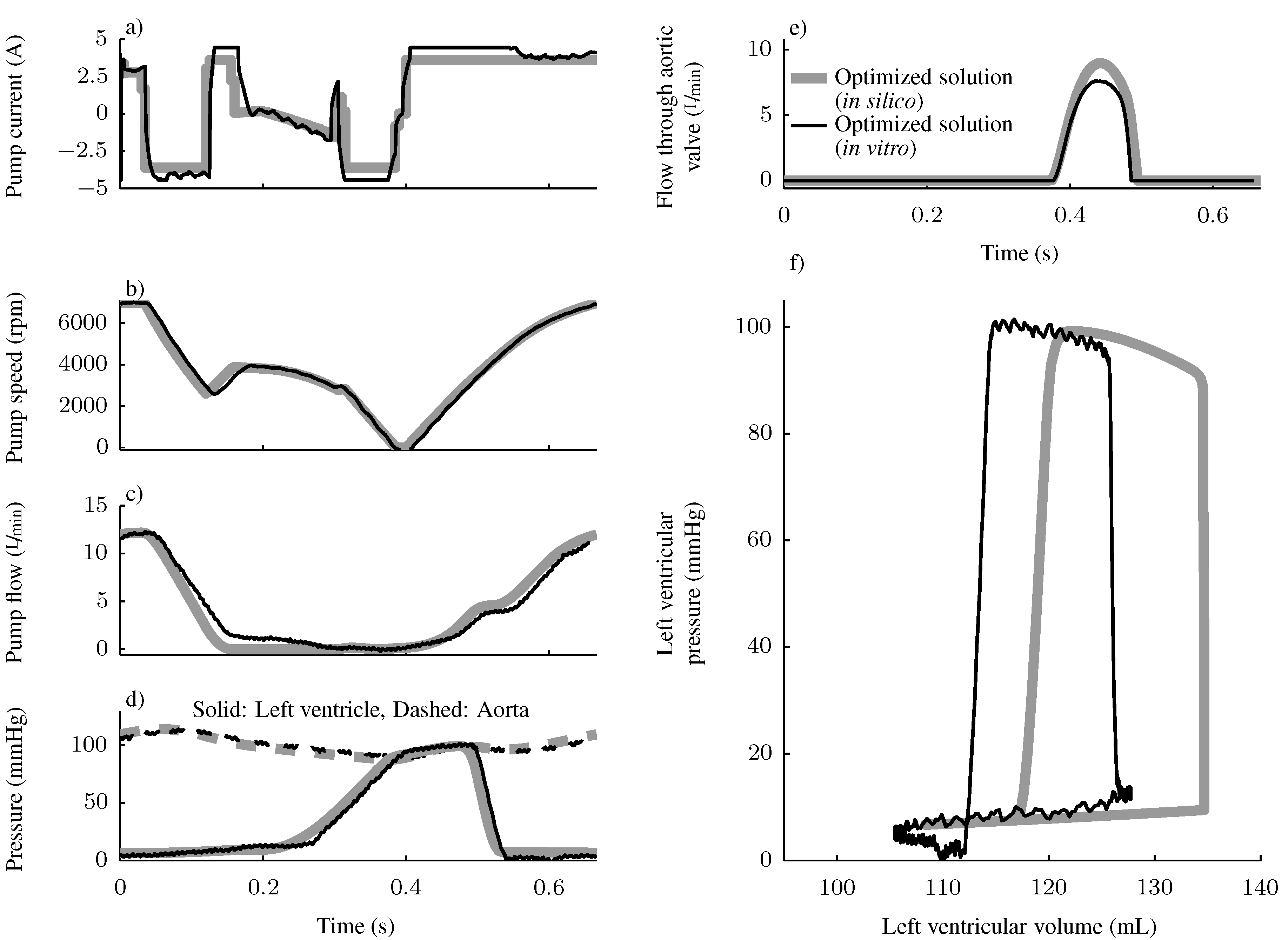
2.3. Validation on the Hybrid Mock Circulation
The hybrid mock circulation presented in [
25] was used to validate one solution resulting from the optimization procedure described in
Section 2.2.4. This test bench interfaces a hydraulic system with the full model that is used for the simulations. The model runs in real time on a PC. The calculated left ventricular and aortic pressures are reproduced by two pressure-controlled hydraulic reservoirs. The mixed-flow blood pump is connected to these reservoirs and, thus, perceives pressures that closely approximate an
in vivo environment. The flow rate through the blood pump is measured using an ultrasonic flow probe (11PXL, Transonic Systems Inc., Ithaca, NY, USA). It is fed back to the circulation model to allow a real-time interaction between the blood pump and the numerical circulation model.
An optimized speed trajectory was realized using a modified speed controller for the blood pump. After several cardiac cycles, stationary operation was reached, as imposed within the OCP by periodicity conditions Equations (
6e) and (
6f). Upon reaching steady state, the data from the last cardiac cycle was stored for further analysis. The pressures in the two reservoirs, representing the up- and down-stream pressures of the blood pump, as well as the pump speed and flow rate were measured. In addition, all relevant data from the numerical simulation were saved along the measured signals.
4. Discussion
In the current study, numerical optimal control was used to optimize the functional interaction between tVADs and the circulatory system. The performance of speed profiles was assessed by a physiologically motivated objective function. A mathematical model was used during the optimization, and the results were validated on a real blood pump in a hybrid mock circulation. This approach yields a better performance than constant-speed or sinusoidal profiles.
The necessity of taking into account multiple physiological constraints simultaneously has been pointed out in previous work [
14]. In that study, bounds were specified for the stroke volume of the left ventricle, for the mean left atrial and ventricular pressures, as well as for the arterial pulse pressure. All results from the optimal-control approach presented in the current paper stay within these bounds. The framework of numerical optimal control can handle any type of constraints imposed on the state variables and the inputs. Whenever certain physiologic measures appear to be out of range, additional constraints can be specified in the OCP. Such constraints would either force the measures in question to stay within the desired limits, or, if no feasible solution is found, an improper selection of these limits would be revealed. This feature highlights the benefits of the methodology presented, inasmuch as it represents a flexible framework where the objective function and the constraints can be adapted to specific requirements.
Figure 6.
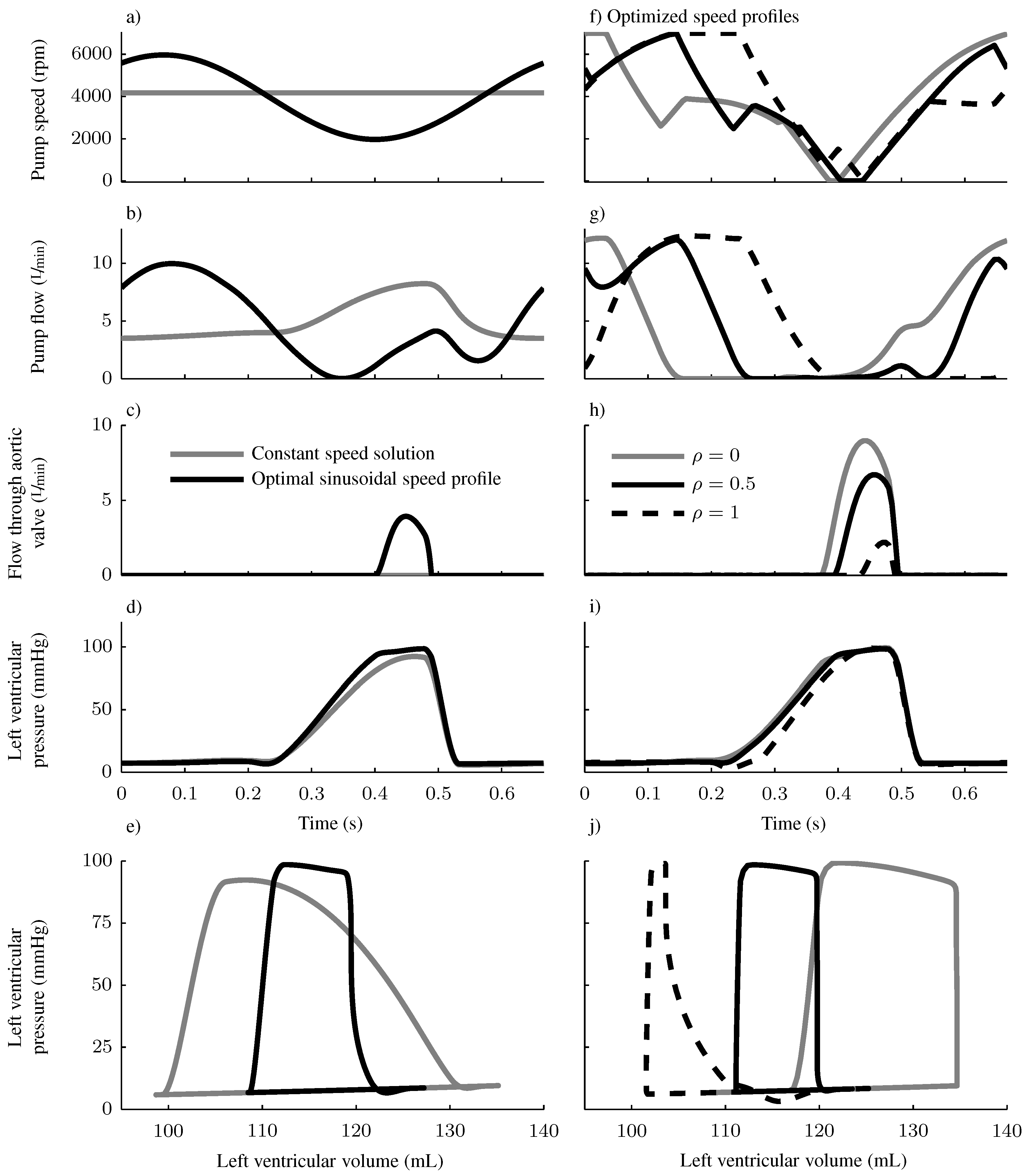
Panels (
a–
e) show the pump speed, the pump flow rate, the flow through the aortic valve, the left ventricular pressure and the left ventricular pressure-volume diagram for the constant speed solution and for the optimal sinusoidal speed profile. The latter is characterized by
,
and
. Panels (
f–
j) show the trajectories of these quantities for the solutions of the OCP with
. For all cases, a value of
is used. The optimized solution with
is equal to the optimized solution (
in silico) shown in
Figure 4.
Figure 6.
Panels (
a–
e) show the pump speed, the pump flow rate, the flow through the aortic valve, the left ventricular pressure and the left ventricular pressure-volume diagram for the constant speed solution and for the optimal sinusoidal speed profile. The latter is characterized by
,
and
. Panels (
f–
j) show the trajectories of these quantities for the solutions of the OCP with
. For all cases, a value of
is used. The optimized solution with
is equal to the optimized solution (
in silico) shown in
Figure 4.
Figure 7.
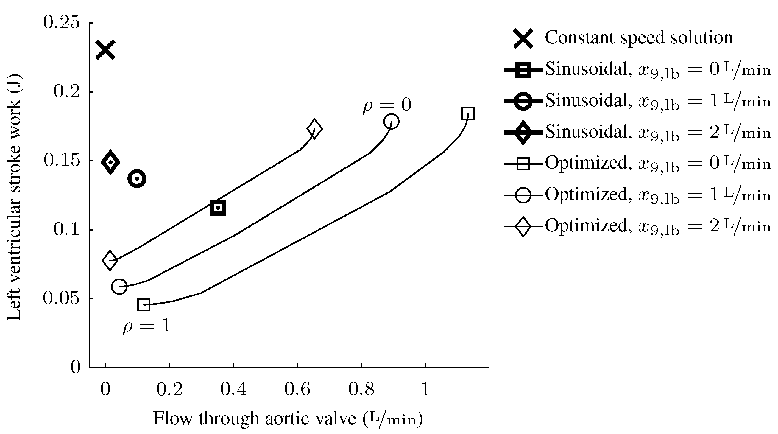
Tradeoff between the flow through the aortic valve and the left-ventricular stroke work. Recall that a higher flow through the aortic valve and a lower stroke work decrease the objective-function value Equation (
6a). Values for the constant speed solution, the optimal sinusoidal speed profiles and the optimal solutions are shown. Three different values for the lower bound on the minimum pump flow rate are applied. The parameter,
ρ, was varied between zero (the flow through the aortic valve is maximized) and one (the left ventricular stroke work is minimized). The optimal parameter set for the sinusoidal profile is invariant w.r.t.
ρ; see
Figure 5.
Figure 7.
Tradeoff between the flow through the aortic valve and the left-ventricular stroke work. Recall that a higher flow through the aortic valve and a lower stroke work decrease the objective-function value Equation (
6a). Values for the constant speed solution, the optimal sinusoidal speed profiles and the optimal solutions are shown. Three different values for the lower bound on the minimum pump flow rate are applied. The parameter,
ρ, was varied between zero (the flow through the aortic valve is maximized) and one (the left ventricular stroke work is minimized). The optimal parameter set for the sinusoidal profile is invariant w.r.t.
ρ; see
Figure 5.
As described in the introduction, numerous approaches exist for speed modulation of tVADs, synchronized or asynchronous to the ventricular contraction and with different types of speed profiles. None of these approaches has been applied clinically as yet, where, normally, a constant speed is applied. The bandwidth of the reference-speed tracking in a real application is important. For example, square-wave speed profiles cannot be tracked exactly, due to the rotor inertia and the limited electric power that is available. When speed profiles are derived from the solution of an OCP, these limitations can be taken into account by the introduction of appropriate constraints.
The OCP Equation (6) is formulated for one cardiac cycle, i.e., it is assumed that the optimal solutions are periodic with the same duration as the cardiac cycle. To verify this assumption, an OCP similar to Equation (6) was solved, where the time horizon included two cardiac cycles. No periodicity constraints were imposed in between these two cycles. The resulting solution was periodic with the duration of only one cardiac cycle, and the speed profiles for the two cardiac cycles were identical.
When such synchronized speed profiles are to be applied in clinical practice, the timing of the ventricular contraction must be extracted from a measured signal, which might require data from an additional sensor, such as from the electrocardiogram [
40]. Similar methods were available in some first-generation, volume displacement VADs [
41]. Potentially, the synchronization of a VAD to the cardiac cycle could be realized using pump-intrinsic signals only by extending the work presented in [
42]. Nevertheless, when speed modulation is to be applied clinically, the option of using optimized speed profiles as presented in the current paper should be considered, due to its superior performance, as indicated in
Figure 7.
The solutions generated by the optimal-control approach are non-causal and rely on an offline, model-based optimization of the pump-speed profile. Two options for realizing their potential in the context of causal control,
i.e., in a clinical application with the possibility for patient-specific treatment, are outlined next.
- (1)
The optimal speed profiles can be parametrized for various physiological states, e.g., various heart rates or changing objective functions. These pre-calculated optimal solutions could then be programmed in a clinical controller. A possible application would be to switch between different speed profiles, including the standard solution where a constant speed is applied. Further research is necessary to verify this approach.
- (2)
Online algorithms could be developed on the basis of the insights gained from the optimal solutions. For example,
Figure 6 reveals that for minimizing the objective function Equation (
6a), a two-step control strategy should be applied: In the first part of the speed profile, the pump speed is chosen, such that the pump flow stays at its lower boundary. In the second part of the speed profile, the pump flow needs to be controlled, such that the desired cardiac output is reached and, therefore, a flow pulse is generated. The parameter,
ρ, thereby adopts the role of a phase shift and varies the timing of the two parts with respect to the ventricular contraction.
Furthermore, the solutions generated by solving an OCP can be used for benchmarking other approaches based on mathematical models. The performance of any control strategy can be compared to the optimal value, which allows one to assess the remaining potential. Finally, a fair comparison among various VAD types can be performed by comparing the optimal behavior of the devices in question.
The optimal pump flow profiles obtained in the current paper are comparable to those typically obtained with a pulsatile volume-displacement VAD, although with a lower amplitude. The effect of the timing of the ejection phase of such a pulsatile volume-displacement VAD on the stroke work and the aortic valve flow was demonstrated earlier
in vivo [
43]. Similarly to the results in the current paper, that analysis shows that a change in phase shift is required when the maximization of the aortic valve flow was assigned preference over the minimization of the left ventricular stroke work.
The blood damage induced by blood pumps represents a complex topic, and different outcomes in this regard have been observed clinically with different types of devices [
44]. Increased hemolysis due to speed modulation has been reported for a commercially available centrifugal pump
in vitro [
45,
46]. Another group designed an impeller to reduce blood damage during speed modulation, which was successfully tested
in vivo [
47,
48]. A recently designed VAD (HeartMate III, Thoratec Corp., Pleasanton, CA, USA) is expected to go into clinical trial soon and employs speed modulation with gradients of up to
[
49]. So far, no mathematical description for blood damage by means of lumped parameter models exists. Therefore, such a description could not be included into the framework presented as yet.
The results shown in the current manuscript demonstrate the potential of the methodology proposed. Future studies should focus on a sensitivity analysis of the optimal solutions. On the one hand, the benefit attainable by the application of optimized speed profiles has to be assessed on a more comprehensive range of the state of the cardiovascular system. On the other hand, the sensitivity of the objective-function value to deviations from a design point used during the optimization should be analyzed. This analysis indicates which physiological parameters need to be included as scheduling parameters in a clinical application. At the same time, the trends of the optimal operating strategy w.r.t. these parameters are revealed, from which guidelines for the development of online control strategies may be derived.
The method presented is able to generate optimal speed profiles for tVADs. By integrating the cardiovascular system into the optimization procedure, this approach not only allows the operation of the tVAD itself to be optimized, but it also improves its interaction with the cardiovascular system. The methodology presented is well suited as a tool for further research of speed modulation for tVADs. Transferring the results obtained to the clinical setting would allow one to adjust the pump performance according to the intention-to-treat of the individual patient, such as the recovery of the native heart or lifelong support.


