
Contributions of Human Activities and Climatic Variability to Changes in River Rwizi Flows in Uganda, East Africa


Department of Civil and Environmental Engineering, Kyambogo University, P.O. Box 1, Kyambogo, Kampala, Uganda
*
Author to whom correspondence should be addressed.
Hydrology 2021, 8(4), 145; https://doi.org/10.3390/hydrology8040145
Submission received: 30 August 2021
/
Revised: 21 September 2021
/
Accepted: 22 September 2021
/
Published: 26 September 2021
Abstract
:This study employed Soil and Water Assessment Tool (SWAT) to analyze the impacts of climate variability and human activities on River Rwizi flows. Changes in land use and land cover (LULC) types from 1997 to 2019 were characterized using remotely sensed images retrieved from Landsat ETM/TM satellites. SWAT was calibrated and validated over the periods 2002–2008 and 2009–2013, respectively. Correlation between rainfall and river flow was analyzed. By keeping the optimal values of model parameters fixed while varying the LULC maps, differences in the modeled flows were taken to reflect the impacts of LULC changes on rainfall–runoff generation. Impacts due to human activities included contributions from changes in LULC types and the rates of water abstracted from the river as a percentage of the observed flow. Climate variability was considered in terms of changes in climatic variables such as rainfall and evapotranspiration, among others. Variability of rainfall was analyzed with respect to changes in large-scale ocean-atmosphere conditions. From 2000 to 2014, the portion of River Rwizi catchment area covered by cropland increased from 23.0% to 51.6%, grassland reduced from 63.3% to 37.8%, and wetland decreased from 8.1% to 4.7%. Nash–Sutcliffe Efficiency values for calibration and validation were 0.60 and 0.71, respectively. Contributions of human activities to monthly river flow changes varied from 2.3% to 23.5%. Impacts of human activities on the river flow were on average found to be larger during the dry (14.7%) than wet (5.8%) season. Using rainfall, 20.9% of the total river flow variance was explained. However, climate variability contributed 73% of the river flow changes. Rainfall was positively and negatively correlated with Indian Ocean Dipole (IOD) and Niño 3, respectively. The largest percentages of the total rainfall variance explained by IOD and Niño 3 were 12.7% and 9.8%, respectively. The magnitude of the correlation between rainfall and IOD decreased with increasing lag in time. These findings are relevant for developing River Rwizi catchment management plans.
1. Introduction
The hydrological cycle of a river basin comprises complex processes which may be impacted upon by climate variability and human activities [1,2,3,4]. It is known that climatic variables especially rainfall and evapotranspiration (ET) are the main determinants of the rainfall–runoff volumes across a catchment. Dynamics of rainfall–runoff generation may be influenced by human-induced changes in land use and land cover (LULC) types. For instance, as explained in [5], anthropogenic influences such as deforestation, overgrazing, and significant expansion of urbanized areas over a given catchment lead to changes in the catchment behavior by (1) affecting the amount of infiltration into the soil, (2) altering the amount and velocity of the overland rainfall–runoff, and (3) modifying the rate and amount of evaporation. Therefore, analysis of the influence of climate variability and human activities on river flow temporal variation is relevant for adaptive planning of water resources management.
The River Rwizi (which drains over 8000 km2 area and is used by communities in at least 12 districts of Uganda, East Africa) has been reported to be undergoing decline in its volume and subsequent drying of wetlands within the catchment [6,7,8]. Deposition of eroded soil might have led to reduced river volume [8]. Concern on the declining River Rwizi can be found reported on several occasions, for instance:
“In the early 1950’s the thick vegetation of papyrus and other wetland grasses around River Rwizi acted as water filters, catchment and regulated flooding in the area. Today, the river, which drains its water into Lake Victoria, is almost lost. Should government fail to eject or prevent further encroachments on the river, the entire Mbarara district will run out of water soon, …” Daily Monitor [6], and “… River Rwizi, a lifeline river for over four million people in southwestern Uganda, has seen up to 80 percent of its water dry up as a result of land taken by individual Ugandans. 200 people have illegally acquired over 500 hectares of land along River Rwizi, destroying wetlands on its banks” Pulitzer Center [9].
Additionally, the rapid urbanization, a condition that is leading to irresistible demand for the water resource, seems to be putting an enormous strain on the River Rwizi flow volume [7,8]. Industrial processes and other commercial activities which rely on the River Rwizi for their water needs are being frustrated. For instance, Nile Breweries Limited receives 10% instead of 75% of the planned water needs. This is likely to discourage potential investors in the region, thereby curtailing economic transformation and efforts to improve livelihoods of communities in the River Rwizi catchment [10].
Changes in river flow can also be influenced by climate variability. Several studies can be found conducted on the variability of rainfall and ET in the region where the study area is located (see e.g., [11,12,13,14,15,16,17]). Variability of rainfall across the tropics is believed to be largely dependent on the latitudinal migration of the Inter-Tropical Convergence Zone (ITCZ). It is also well known that rainfall variability over the equatorial region where the study area is located is driven by the El Niño Southern Oscillation and the Indian Ocean Dipole (IOD) (see e.g., [18,19,20]). Influences of the changes in large-scale ocean-atmosphere conditions on the variability of temperature and PET can be inferred from the drivers of rainfall [21]. In East Africa, regional atmospheric dynamics and stability are also controlled by the combined effects of the influences from the high mountains (Mount Rwenzori, Mount Kenya, Mount Elgon, and Mount Kilimanjaro) and the Great Lakes (Lake Victoria, Lake Tanganyika, and Lake Malawi) [22].
To the best of our knowledge, there has never been any study to specifically quantify the contributions of climate variability and human activities to the variation on River Rwizi flows or rainfall–runoff across the River Rwizi catchment. Eventually, the purpose of this study was to fill the said knowledge gap. To do so, the specific objectives of this study were to (i) characterize LULC changes in the River Rwizi catchment, (ii) model and simulate River Rwizi flow changes using a semi-distributed model, (iii) quantify the amount of change in River Rwizi flow attributable to the impacts of human activities, and (iv) quantify the extent to which River Rwizi flow is driven by climatic variability.
2. Materials and Methods
2.1. Study Area
The River Rwizi catchment, which has a drainage area of 8554.7 km2 and lies between longitudes of 30.21° E to 32.52° E and latitudes of 0.24° S to 0.92° S, is located in the south-western Uganda. It has the River Rwizi, which flows through more than 12 districts in the western region including Mbarara, Sembabule, and Ntungamo, among others [23]. River Rwizi originates from the hills found in the western Uganda and has a series of tributaries joining it as it flows in the southern direction (Figure 1a). The river flows eastward for about 57 km until the gauge at Mbarara water works before it joins the River Kagera. It finally discharges its waters into the Lake Victoria. The gauged part of the catchment (gauge station in Mbarara) is approximately 2100 km2 in catchment area (Figure 1a), encompassing portions of six districts including Bushenyi and Mbarara, among others.
The altitude of the Rwizi catchment varies from 1166 to 2171 m above sea level. River Rwizi is the source of water for livelihood for both people and animals covering the Mbarara–Masaka dry corridor including Mbarara, Kiruhura, Lyantonde, Sembabule, Lwengo, Kyotera, and Rakai districts in the eastern and northern sides. In the south, it takes approximately half of Isingiro and three quarters of Rwampara districts towards Tanzania [23]. On the western side, the catchment covers the districts of Ibanda, Buhweju, Bushenyi, Mitooma, and Ntungamo. Rwizi catchment rainfall records show a bimodal pattern with two rainy seasons which occur from March to May and from September to November.
The LULC is highly dominated by agricultural lands (both subsistence and commercial), grasslands due to national parks, forests (natural dense, moderate, sparse, and planted forests), settlements (urban and rural setups), wetlands/swamps, and water bodies (lakes and rivers). Most parts of the catchment are degraded by deforestation, overgrazing and poor agricultural practices. There are several human activities across the River Rwizi catchment and at riverbanks including cattle rearing, brick making, and agroforestry (mainly eucalyptus) [23]. Since River Rwizi catchment experiences environmental changes and, thus, it is important to evaluate variability in its river flows [23].
Based on properties such as clay content, sand content, loam content, and hydrological group, soils in the Rwizi catchment are clay loam, sandy clay loam, loam, sandy loam, and some peat loamy soils. According to Food and Agriculture Organization (FAO) classifications, soils in the Rwizi catchment are the Alisol and Arenic with extremely low base saturations. According to Soil and Water Assessment Tool (SWAT) database, soils in Rwizi belong to Group A—Arenic qualifier (Swanton), Group B—Loamic qualifier (Benson), and Group C—Clayic qualifier (Water) (Figure 1b).
2.2. Data
2.2.1. River Flow
Daily river flow time series running from 2000 to 2013 observed at Rwebikoona, Mbarara Municipality along Mbarara–Ishaka road (River Gauging Station No. 81224) was obtained from Directorate of Water Resources Management of Uganda.
2.2.2. Meteorological Series
To apply the Soil and Water Assessment Tool (SWAT), a number of climatic series, such as temperature and solar radiation, are required. Due to lack of observed meteorological series required by SWAT, the National Centers for Environmental Prediction’s (NCEP’s) Climate Forecast System Reanalysis (CFSR) daily series [24] including rainfall, maximum and minimum temperature, relative humidity, solar radiation, and wind speed were obtained in a gridded (0.25° × 0.25°) form for the period 2000–2013 via http://globalweather.tamu.edu/ (accessed on 3 February 2020).
Other sources of data were also considered to determine the best rainfall series for driving SWAT. In this line, daily rainfall (mm/day) series of the Japanese 55-year Reanalysis (JRA-55) [25], and Climate Hazards group InfraRed Precipitation with Stations (CHIRPS) version 2.0 (or CHIRPS v2.0) [26] were considered. The data for JRA-55 (1° × 1° grid) and CHIRPS v2.0 (0.25° × 0.25° grid) were over periods 1958–2017, and 1979–2013, respectively. Furthermore, we used monthly rainfall of the Climatic Research Unit (CRU) Version 4 time series over the period 1901–2019 [27] and CenTrends v1.0 time series from 1900 to 2014 [28].
Observed daily rainfall at Mbarara Meteorological Station (ID 90300030) over the period 1930–1995 was obtained from the Uganda National Meteorological Authority.
2.2.3. Spatial Data
Digital Elevation Model (DEM) at a resolution of 1 arc second (30 m × 30 m) was retrieved from the United States Geological Surveys (USGS) via https://lta.cr.usgs.gov (accessed on 5 January 2020). The DEM was used for: (i) automatic delineation of the catchment, (ii) defining the stream network, and (iii) establishing sub-basin parameters such as stream network, longest reaches, and drainage surfaces and slope.
LULC information was obtained from remotely sensed images retrieved from USGS Landsat ETM/TM satellites via http://www.earthexplorer.usgs.gov/ (accessed on 18 January 2020) in Path 171 and Row 60 at a spatial resolution of 30 m. The images for the years 1997, 2000, and 2008 were obtained from Landsat 7. Recent LULC types for years 2014 and 2019 were obtained from Landsat 8 (which is the now decommissioned Landsat 5).
The soil map was obtained from Land and Water Resource, FAO soil database [29] at a scale of 1:5,000,000. Details on the soil map can be obtained via http://www.fao.org/soils-portal/soil-survey/soil-maps-and-databases-FAOUNESCO-soil-mapoftheworld/en/ (accessed on 23 January 2020).
2.3. Methods
2.3.1. Analysis of the LULC Changes
Landsat images were classified into six LULC types. The LULC types included agricultural or cropland, settlement (built-up areas including both urban and rural setups), forests (dense, moderate, sparse, and planted), water (lakes and rivers), wetlands (swamps and papyrus), and grasslands. We focused on the area covered by each LULC type from a given classified map. This was important to determine which LULC type was increasing or decreasing over time.
2.3.2. SWAT Modeling and Quantification of Human Impacts
- I.
- Selection of rainfall series to use for modeling
The observed river flow and rainfall were over different periods 2002–2013 and 1930–1995, respectively. Thus, observed rainfall could not be used for the hydrological modeling. Correlation between the observed river flow and reanalysis rainfall was analyzed to determine the most suitable rainfall series for driving SWAT. Climatic data from the study area was found to exhibit strong seasonality and this would affect results of correlation analysis. Thus, to avoid the influence of the seasonality, correlation was analyzed separately for each month. In other words, coefficients of correlation between river flow and reanalysis or satellite-based rainfall over the period 2002–2013 was computed separately for the sub-series of each month.
- II.
- SWAT model build-up and sensitivity analysis
Rainfall–runoff was modeled using SWAT 2012 version based on the water balance equation [30].
where, n = sample size, SWi = final soil water content (mm) for the ith day or month depending on the time scale used for modeling, SWo = initial soil water content (mm), Rday = rainfall (mm), Qsurf = surface runoff (mm), Qgw = amount of return flow (mm), ET = evapotranspiration (mm), and Wseep = amount of water (mm) entering the vadose zone from the soil profile (soil interflow).
The procedure for the model build-up comprised catchment delineation using DEM, division of sub-basins into smaller units called hydrologic response units (HRUs) based on both DEM and soil information, and importing weather data into the model. The model was run on a monthly scale over the period 2000–2008. The first two years were used as the warm-up period. SWAT has so many model parameters and it would be arduous to simultaneously change all of them during a single calibration. Thus, a few sensitive parameters were required to be identified for calibration. In this study, sensitivity analysis was performed using the global approach in semi-automated Sequential Uncertainty Fitting (SUFI2) algorithm [31]. The most sensitive parameters were selected based on Student t-statistics and p-values from the sensitivity analysis. Finally, SWAT inputs and outputs were assessed based on the information from Arnold et al. [32].
- III.
- SWAT model calibration and validation
Calibration and validation were performed over the periods 2002–2008 and 2009–2013, respectively. Calibration and validation of SWAT was based on the LULC map for 1997. Evaluation of model performance during calibration and validation was performed both graphically and statistically. Graphically, plots of observed versus modeled series were made. Statistically, model performance was assessed using Nash–Sutcliffe Efficiency (NSE) [33], coefficient of determination (R2), and percentage of bias (Pbias) such that
where n is the sample size, denotes the ith observed value, represents the ith modeled value, while and are the mean values of the observed and modeled series, respectively. NSE varies from negative infinity to one. Values of R2 occur from zero to 1. Application of R2 is based on the assumption that observed and modeled series are linearly related [34].
- IV.
- Simulations and LULC change impacts
There are a number of ways to investigate impacts of LULC changes on hydrology. In case of a step jump in flow mean, analysis is conducted on whether changes in LULC types before and after the change point can be linked to the respective flow characteristics (see, e.g., Pirnia et al. [4]). We can also apply the hydrological sensitivity elasticity-based method to investigate river flow sensitivity to rainfall and ET. To do so, we make use of the dryness index and plant available water coefficient (see e.g., [35,36]). In some cases, we focus on rainfall elasticity or relating the amounts of change in rainfall to that of river flow (see e.g., [37,38]). In a scenario analysis, changes can be made to the LULC type(s) while the hydrometeorological model inputs over the study period are kept unaltered. With such a scenario analysis, we can determine the amount by which river flow will change when, for instance, a given percentage of forest is converted to cropland while other LULC types remain unaffected. In another approach, the study period is divided into a number of sub-periods. Over each sub-period, we can have a separate LULC map. The (semi)distributed model is run over each sub-period. Note is taken on whether changes in some relevant parameters like the curve number over the various sub-periods can explain the variation in flow property. This approach was applied to investigate impacts of LULC changes on water availability of Tons River Basin, Madhya Pradesh, India [39]. Without LULC maps, a conceptual model can be run over the various sub-periods, and changes in each of the relevant parameters related to LULC information can be analyzed (see e.g., [40]).
It becomes too complex to quantify impacts of LULC types on hydrology if the synergistic influences from other factors (such as limitation of the model, and climate variability) are not controlled during the simulation experiment. Thus, it is expected that the simulated river flow series obtained when the model is driven by LULC maps for 2000, 2008, 2014, and 2019 would be the same so long as:
- (1)
- The optimal set of model parameters is kept constant during each simulation;
- (2)
- The same hydrometeorological series (such as rainfall and potential ET series) are used as model inputs over the given study period; and
- (3)
- There are no differences among the LULC maps (in other words, the spatial information from LULC maps for 2000, 2008, 2014, and 2019 are totally the same).
To determine the impacts of LULC changes on hydrology, we assume that conditions (1) and (2) are true while (3) is false. Thus, there were four simulations, one based on the LULC map of 2000 and the others using LULC maps for 2008, 2014, and 2019. During each simulation, soil information remained spatially the same as that used during calibration and validation. The absolute difference between the means of model outputs over the period 2002–2013 based on LULC maps 1997 and 2000 (as a percentage of the mean of modeled series based on LULC map 1997) was considered to be due to the changes in LULC types from 1997 to 2000. The same procedure was taken to determine impacts of LULC changes for the periods 1997–2008, 1997–2014, and 1997–2019.
- V.
- Impacts of human activities and climate variability
The procedure to quantify impacts of human activities and climate variability was as follows:
- (a)
- As explained shortly above, the differences in the model results based on LULC map of 1997 and the simulations of LULC maps for 2000, 2008, 2014, and 2019 were taken to reflect the impacts of LULC changes on rainfall–runoff generation across the catchment.
- (b)
- To the differences in the means of the model results from (a), water diverted from the river through other human activities especially abstraction to supply several towns and industries within the catchment was added and the overall result was expressed as a percentage of the mean of observed flow.
- (c)
- The amount of total variance in river flow explained by the rainfall was computed. It is worth noting that rainfall–runoff generation is also controlled by other factors such as infiltration, percolation, and variation in evapotranspiration. Thus, if we assume that the model is perfect (or nearly so), the percentage of total variance in the observed flow explained by the simulated river flow indicates the influence of the other factors (like infiltration and percolation) and variation of climatic conditions (including changes in rainfall, temperature, and evapotranspiration) on rainfall–runoff generation.
- (d)
- The remaining percentage after deducting the total contribution from human activities (or LULC changes and river flow abstraction) and the percentage of the total river flow variance explained by the simulated flow (or an indicator of the influence of climate variability) was attributable to other factors such as reduced capacity of the hydrological model to capture complexities in rainfall–runoff generation processes, and possible flow returns into the river through discharge of effluents from industries.
2.3.3. Analysis of the Rainfall Variability
Insight on the linkage of variability of river flow and rainfall to the changes in large-scale ocean-atmosphere conditions was investigated using correlation analysis. Coefficients of correlation between river flow or catchment-wide averaged rainfall and two climate indices including Niño 3 index [41,42] and the IOD index were analyzed. The IOD index refers to the anomalous sea surface temperature (SST) difference between the western (50° E to 70° E and 10° S to 10° N) and the southeastern (90° E to 110° E and 10° S to 0° N) equatorial Indian Ocean. The Niño 3 refers to the SST across the tropical Pacific region (90°–150° W and 5° N–5° S). Before correlation analysis, seasonal components of the rainfall and river flow were removed. The steps to remove seasonality from the series involved [43] (a) extracting rainfall or flow for each month, (b) computing the long-term mean of the series extracted in (a) for each month, (c) taking the long-term monthly mean pattern as the seasonal model for each year of the data record, and (d) subtracting the long-term mean of a given month from the corresponding original data value.
3. Results and Discussion
3.1. LULC Changes in Rwizi Catchment
Figure 2 shows the results of the LULC classifications. Visually, the two dominant LULC types based on each map were grassland and cropland (Figure 2a–e). Results of computed areas of the various LULC types can be seen in Table 1 and Table 2. The smallest portion of the catchment area in each year was taken up by settlement.
Graphical results on the transition in the LULC types can be seen in Figure 2f. It is important to note that the vertical axis was plotted on a logarithmic scale to reduce the large disparity in the orders of magnitudes for clarity. From 1997 to 2019, grassland was characterized by a decreasing trend. However, forest and settlement areas exhibited increasing trends at rates of 2187 and 1332 ha/year, respectively. This means that the decrease in grassland was due to the population increase. While grassland was decreasing at a rate of −9260 ha/yr, cropland was characterized by a positive trend with magnitude of 3083 ha/yr. Due to the population increase, large areas of grassland were converted to farmlands or grazing lands.
In 1997, LULC comprised grassland (54.7%), cropland (38.2%), forest (1.7%), wetland (3.5%), water (1.8%), and settlement (0.1%) of the catchment area (Table 1). Generally, it is noticeable that some LULC types were increasing while others were decreasing over time. By 2019, grassland and cropland had reduced to 36.6% and 31.6%, respectively. However, forest increased to 9.8%. Settlement increased from 0.1% to 4.8% over the period 1997–2019. From 2000 to 2014, wetland reduced in area from 8.1% to 4.7%. One main reason for the decrease in wetland was due to the massive illegal acquisition of land along the River Rwizi [9].
Generally, the amount by which a particular LULC type changed depended on the selected period (Table 2). For instance, the largest increase in cropland was over the period 2014–2019 followed by 1997–2000. However, grassland increased and decreased over the periods 1997–2000 and 2000–2019, respectively. The differences in the changes of LULC types over the periods reflect the influences of the various key land laws of the Republic of Uganda [44,45,46,47].
3.2. SWAT Modeling
3.2.1. Correlation Analysis
Table 3 shows results of the correlation between river flow and rainfall. For all the rainfall products, negative correlation was found for the sub-data of at least one month. CRU data was negatively correlated with river flow for most of the months. Except for July, CFSR rainfall was positively correlated with river flow of the various months. Negative correlation coefficients were in the sub-series of July and August (for CHIRPS) or February, April, and August (in JRA55). CenTrends exhibited negative correlation with river flow sub-series of October.
Without considering the influence of lag in time, the amount of variance in flow, which could be explained by the CFSR rainfall, varied from 0.35% (in June) to 45.62% (for September). For other rainfall products, the explained percentages of the total river flow variance varied over the ranges 0.08–34.17%, 1.63–58.44%, 0.00–12.50%, and 1.58–26.14%, for CRU, CHIRPS, JRA55, and CenTrends, respectively. Considering all the months, the averaged percentages of the total variance in river flow explained by CFSR, CRU, CHIRPS, JRA55, and CenTrends were 20.94%, 8.69%, 16.36%, 2.84%, and 10.26%, respectively. This meant that CFSR was the best rainfall product for possible hydrological modeling over the study period.
Considering 1-month lag, coefficients of correlation between CFSR and river flow were higher in magnitude for January, July, and November than in the case with zero lag. For the other months, correlation coefficients were less in magnitude when 1-month lag was considered than in the case with zero lag. This indicates that the speed with which the catchment as a system responds to the rainfall input is moderate. How fast a catchment responds to rainfall input depends on a number of factors such as catchment area, influence of human activities, geology and soil, etc.
Figure 3 shows monthly rainfall in the study area. Observed data was based on observations from Mbarara meteorological station (ID 90300030). For other datasets (CenTrends, CRU, CHIRPS, CFSR, and JRA55), catchment-wide averaged rainfall was used. It is noticeable that the observed bimodal pattern of rainfall was adequately reproduced by data from various sources (Figure 3a–e) although there are some under-estimations or over-estimations.
For the CFSR data (Figure 3a), the rainfall total of each month was larger over the recent (2002–2013) than that of the long-term (1979–2015) period. For the CenTrends and CRU data, it is for the sub-series of October, November, and December that the recent (2002–2013) rainfall totals were greater than those of the long-term (1901–2015) period (Figure 3b,c). For the CHIRPS data, recent (2002–2013) rainfall totals were greater than those for the long-term (1981–2019) period in the months of February, March, April, May, June, August, and September. Results obtained using the JRA55 (Figure 3e) contrasted those for other datasets (Figure 3a–d). In other words, JRA55 showed that recent (2002–2013) rainfall totals were less than those for the long-term (1958–2017) period. Nevertheless, all the datasets from the various sources generally show that the study area’s rainfall is of a bimodal pattern or there are two wet sub-periods in each year including March–April–May (MAM) and September–October–November–December (SON) rainy seasons. January–February (JF) and the June–July–August–September (JJA) months are the short and long dry seasons, respectively.
3.2.2. SWAT Model Results
There were 1145 HRUs in 29 sub-basins obtained following the watershed delineation. The smallest and largest sub-basins in the catchment were 13.2 km2 and 840.4 km2, respectively. After LULC reclassification based on SWAT database, six classes were obtained, namely, FRST—Forest, AGRL—Cropland, WATR—Water, URBN—Settlement, WETL—Wetland, and PAST—Pasture and Grasslands.
There were eight sensitive parameters which yielded p-values less than α = 0.05 (Table 4). The top four most sensitive parameters were ALPHA_BF (base flow alpha factor, days), HRU_SLP (average slope steepness, m/m), CN2 (moisture condition II curve number), and GWQMN (threshold water level in shallow aquifer for base flow to occur, mm).
The values of NSE, R2, and Pbias for calibration were 0.60, 0.68, and −0.18%, respectively. For validation, NSE, R2, and Pbias were 0.71, 0.71, and −0.04%, respectively. Considering the full time series (combining both calibration and validation data), the statistical metrics NSE, R2, and Pbias were 0.71, 0.73, and −0.10%, respectively. From these statistical performance measures, it can be noted that the model was satisfactory for further application to estimate impacts of the LULC changes and climate variability on rainfall–runoff across the study area.
Figure 4 shows comparison of observed and modeled series. The time series (Figure 4a) and scatter (Figure 4b) plots show that the variation in observed flow was comparable with that in modeled series. However, there was a large mismatch between observed and modeled flow especially at the beginning of the calibration period especially before 2003. Such a large mismatch indicated reduced capability of the CFSR data in reproducing the rainfall, which led to the peak river flows in 2003.
3.3. Possible Large-Scale Drivers of Rainfall Variability
Figure 5 shows variation of correlation between river flows or catchment-wide averaged CFSR rainfall and climate indices at various lags in time. Coefficients of correlation between river flow and CFSR rainfall were positive at all considered lags. However, the highest correlation (0.47) was obtained when there was no lag in time. This, as mentioned before, indicates that the response of the River Rwizi catchment to the rainfall input may range from fast to moderate. Apart from rainfall, other climatic factors such variation in evapotranspiration rates are important in determining river flow variation. Like flow, rainfall was positively and negatively correlated with IOD and Niño 3, respectively. The magnitude of the correlation between rainfall and IOD decreased with increasing lags. The highest correlation between rainfall and IOD was also obtained when there was no lag in time. However, the largest magnitude of the correlation between rainfall and Niño 3 was obtained at the 8-month lag. The largest percentages of the total rainfall variance explained by IOD and Niño 3 were 12.7% and 9.8%, respectively. When IOD and Niño 3 were used as predictors in a combined way through multiple linear regression, up to about 40% of the total variance in rainfall across the equatorial region (where the study area is located) could be explained [48]. Thus, synergies among suitable indicators of large-scale ocean-atmosphere conditions should be considered in investigating predictability of the rainfall variability across the equatorial region. Given that (i) rainfall is correlated with climate indices, and (ii) rainfall is positively correlated with river flow, it means that river flow variability can be inferred from the drivers of temporal changes in rainfall.
3.4. Influence of Human Activities and Climate Variability
Figure 6 shows rainfall and results of simulations. The differences among the simulations from the various LULC maps were not large (Figure 6a). This was an indication that contribution of human activities to the rainfall–runoff variation in the study area was not large. Rainfall especially for the rainy season was characterized by an increasing trend over the study period (Figure 6b). River flow also exhibited an increasing trend over time. This also suggested that the increasing trend in river flow could be due to the increasing rainfall (Figure 6a,b). What cannot escape a quick notice is that, during dry seasons, rainfall remained low. For each year, the river flows during the dry season were much reduced compared to those from wet seasons. These results indicate that the River Rwizi is characterized by large intermittency in river flows. In other words, the difference between flows during rainy and dry seasons in each year is large.
Correlation between CFSR rainfall and river flow was 0.47. However, correlation between modeled and observed flow was 0.85. In other words, the percentage of the total river flow variance that was explained by the modeled flow (considering both calibration and validation results using LULC map of 1997) was 73%. This indicated that river flow variation is influenced not only by rainfall but also other factors which affect infiltration rate, percolation rate, and variation in temperature or evapotranspiration, among others.
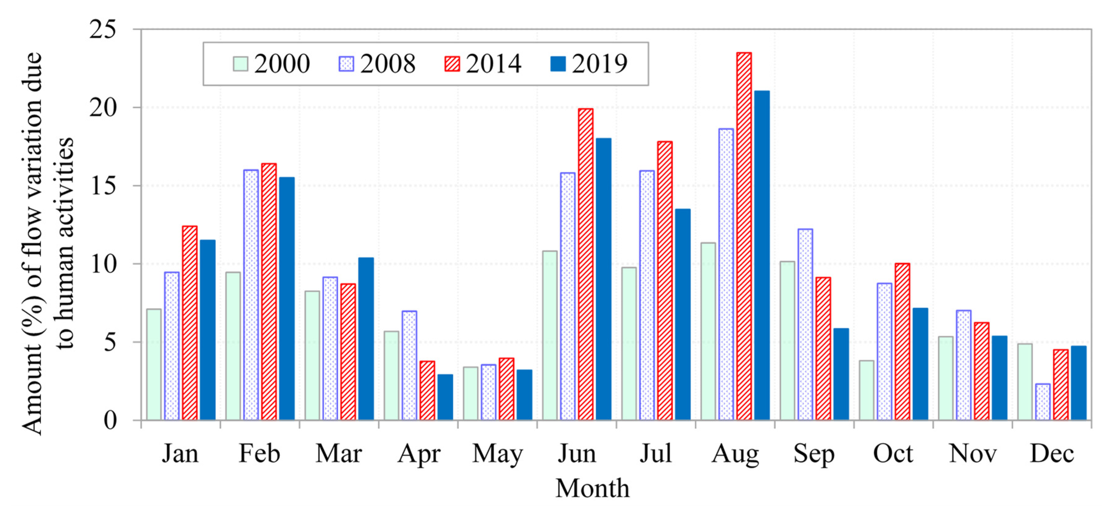
Figure 7 shows the response of rainfall–runoff to impacts of human activities based on the various LULC maps. Amount of influence of human activities on rainfall–runoff varied from one month to another. This reflected the variation in the human activities, for instance, with rainfall season. For instance, some activities such as planting of crops are ceased during the rainy season. Bush clearing and burning tends to occur during the dry season.
Generally, contributions of human activities to rainfall–runoff variation went up to 23.5% in August. For wet seasons (March–April–May, and October–November–December, amounts of contributions of human activities to river flow variation remained low. On average, the contributions from human activities to the monthly river flow variation over the periods 1997–2000, 1997–2008, 1997–2014, and 1997–2019 were 7.5%, 10.5%, 11.4%, and 9.9%, respectively.
The River Rwizi has been reported to be dwindling due to impacts of human activities on the hydrology of the catchment [6,7,8,9,10]. A research study was required to determine whether the impacts of human activities could be as substantial as reported by the media. Our study indicated that the mean River Rwizi flow over the study period exhibited an increasing trend. Positive trend in each month was found to be positive. River flows of January, April, June, August, October, and November as well as that of the annual time scale exhibited significant (p < 0.05) increasing trends. Increasing trends were also found for the rainfall of each month. These results indicated that, given the increasing rainfall, the impacts of human activities across the River Rwizi catchment did not alter the direction of trends in the flows over the period 2000–2013. At least 73% of the variation in the mean rainfall–runoff across the study area could be attributable to the impacts of climate variability on hydrology. The amounts of contribution of human activities (especially from changes in LULC types and river flow abstraction) to variation of the River Rwizi flow over the period 1997–2019 varied over the range 2.3–23.5%. However, the impacts of human activities on the river flow were on average found to be larger during the dry (14.7%) than wet (5.8%) season. Considering both dry and wet seasons, the contributions of the human activities to the variation in river flow was 9.8% on average. The increasing pressure from the rapidly growing population in terms of activities such as encroachment of wetlands (through planting of eucalyptus in wetlands and sand mining), and massive water abstractions especially during the dry season could be responsible for making the River Rwizi catchment hydrologically drier than it would be if it was minimally impacted upon by human activities or when allowed to exist under natural conditions.
Explanation of why there is reduced effect of human activities on the river flow of wet period could be given in terms of information theory and content in the forcing (rainfall). It is worth noting that a system can be defined in its internal and external components. Significant external force on a system (which is a catchment in this case), for instance through heavy rainfall over longer period (wet period), suppresses the effect of internal processes in the system output. However, when the system forcing is much reduced in magnitude (for instance, dry period or minimal amount of rainfall), the system’s internal processes (such as infiltration rates which can easily be affected by human activities like deforestation) will have a more pronounced effect on the output. Some of the relevant literature on concepts regarding analysis of the effect of forcing on the systems in the context of hydrological modeling can be obtained from [49,50,51,52].
The impacts of human activities on the rainfall–runoff variation was larger based on the LULC map of 2014 than that of 2019. This suggests that that there was some reduction in the rate of vegetation and wetland degradation especially after 2014. This could have followed the constant concerns on the need to stop further degradation and wetland encroachment along the River Rwizi. We think that drastic steps by the National Environment Management Authority with the support of Ministry of Water and Environment and Government of Uganda in line with the need for restoration of the River Rwizi especially after 2014 could have reduced the negative impacts of human activities on the hydrology of the catchment.
Notably, our results are based on flows aggregated to a monthly scale. We think that more realistic results could be obtained by modeling rainfall–runoff using data of high temporal resolution such as daily or hourly series. This requires high quality observed data for the study area and this, as we found during our study, is still a challenge.
Regulations on water abstractions especially during dry season should be carefully enforced to ensure sustainability of the water resources in the catchment. One way would be to set and maintain a threshold water abstraction rate that ensures that the catchment hydrology supports functionality of the various water-related or water-based systems. Currently, the regulation of the Ministry of Water and Environment of Uganda ensures that Q90 (or the flow which is exceeded 90% of the times the flows is recorded over a stipulated period) or Q95 is used as the environmental flow especially in absence of a relevant study. The question would be whether water abstractors or users adhere to the environmental flow given the disproportionate volumes of water abstracted by the various permitted and unpermitted water users. As opposed to the use of Q90 or Q95, the threshold for water abstraction could be set while taking into account (i) the dynamics of rainfall–runoff generation in the various sub-flows (baseflow, interflow, and overland flow) given the variation in rainfall and ET across the study area, and (ii) level of adherence to the environmental flow by the various water abstractors.
Contributions from human activities and climate variability to river flow changes were 9.9% and 73%, respectively. Contributions from other factors to the variation in river flow totaled 17.1% (i.e., 100–9.9–73). The remaining or unexplained 17.1% of the total variability in river flow could be due to (i) limited capacity of the hydrological model, and (ii) extra impacts of human activities such as flow returns into the river through discharge of effluents from industries, and unpermitted water abstractions not included in the abstraction data used in this study. Reduced capacity of the hydrological model can be due to a number of reasons including (a) inaccuracies in parameters of the model, (b) imperfection of model structure, (c) observation errors on the river flow against which calibration is to be made, and (d) measurement errors on meteorological model inputs (such as rainfall), and (e) deficiency in characterization and procession of spatial model inputs. In some cases, the factors which reduce the model’s efficacy interrelate with one another. For instance, the best performing parameter vector can be significantly affected by observational or measurement errors [49].
4. Conclusions
This study quantified contributions of climate variability and human activities to the rainfall–runoff variation in the River Rwizi catchment. Changes in LULC types were characterized using Landsat images for 1997, 2000, 2008, 2014, and 2019. SWAT was driven by CFSR-based hydro-meteorological series including rainfall, maximum and minimum temperature, relative humidity, solar radiation, and wind speed. SWAT was built up, calibrated, and validated using the LULC map of 1997. Calibration and validation of SWAT were performed on a monthly time scale over the periods 2002–2008 and 2009–2013, respectively. To depict the transition in LULC changes, SWAT was parameterized using optimal parameter values obtained during calibration and this was followed by simulations based on LULC maps of 2000, 2008, 2014, and 2019.
Over the study period (1997–2019), there was an increase in cropland and settlement by 26.09% and 0.35% of the catchment area, respectively. Wetland reduced by 1.62%. However, grassland decreased by 25.81% of the catchment area. The percentages of the catchment area covered by cropland in 2000 and 2014 were 23.0% and 51.6%, respectively. Grassland covered 63.3% and 37.8% of the catchment area in 2000 and 2014, respectively.
However, wetland covered 8.1% and 4.7% of the catchment area by 2000 and 2014, respectively. These results depicted the pressure of the increasing population on the catchment environment.
Performance of SWAT was deemed to be satisfactory with Nash–Sutcliffe Efficiency values of 0.60 and 0.71 for calibration and validation periods, respectively. Rainfall variability explained 20.9% of the total river flow variance over the period 2002–2013. Contributions of human activities in terms of LULC changes and water abstractions to the river flow variability varied among months and ranged from 2.3% to 23.5%. On average, human activities contributed to the monthly river flow variability by 7.5%, 10.5%, 11.4%, and 9.9% over the periods 1997–2000, 1997–2008, 1997–2014, and 1997–2019, respectively. Impacts of human activities on the river flow were on average found to be larger during the dry (14.7%) than wet (5.8%) season. Therefore, water abstraction (and other human activities which reduce water volumes) during the dry season as well as wetland encroachment should be regulated to ensure normal functionality of various water-related or water-based systems.
Contributions from climate variability to river flow changes was up to 73%. Other factors contributed 17.1% of the river flow variance. For the River Mpanga catchment within the same region where the study area is located, flow variance was due to LULC (8%), climate variability (70%), and other factors (22%) [53]. These findings show that river flow temporal changes in the study area are substantially driven by climate variability. In this study, rainfall was found to be positively and negatively correlated with IOD and Niño 3, respectively. However, correlation between rainfall and IOD decreased in magnitude with increasing lags in time. IOD and Niño 3 explained up to 12.7% and 9.8% of the total rainfall variance, respectively.
In this study, rainfall–runoff generation was simulated using different LULC maps while keeping values of optimal model parameters fixed and the differences in the resulting simulations were taken to reflect impacts of LULC changes on river flow. However, since rainfall can, to some extent, be impacted by characteristics of land surface, we recommend a future study to investigate possible inconsistencies among model fields introduced in results of simulations due to changing LULC maps while using the same rainfall input.
Author Contributions
C.O.: Conceptualization, data curation, formal analysis, investigation, methodology, supervision, validation, writing—review and editing; R.N.: Conceptualization, data curation, formal analysis, investigation, methodology, validation, writing—review and editing. A.N.: investigation, supervision, writing—review and editing. All authors have read and agreed to the published version of the manuscript.
Funding
This research study received no funding.
Institutional Review Board Statement
Not applicable.
Informed Consent Statement
The data used in this study can be freely accessed.
Data Availability Statement
The data used in this study can be freely accessed.
Acknowledgments
The authors acknowledge that this paper was partly from a study by Nyesigire [54] under the supervision of Charles Onyutha and Anne Nakagiri.
Conflicts of Interest
The authors declare that there are no conflicts of interest.
References
- Zhao, G.; Tian, P.; Mu, X.; Jiao, J.; Wang, F.; Gao, P. Quantifying the impact of climate variability and human activities on streamflow in the middle reaches of the Yellow River basin, China. J. Hydrol. 2014, 519, 387–398. [Google Scholar] [CrossRef]
- Wang, F.; Hessel, R.; Mu, X.; Maroulis, J.; Zhao, G.; Geissen, V.; Ritsema, C. Distinguishing the impacts of human activities and climate variability on runoff and sediment load change based on paired periods with similar weather conditions: A case in the Yan River, China. J. Hydrol. 2015, 527, 884–893. [Google Scholar] [CrossRef]
- Huang, H.; Han, Y.; Cao, M.; Song, J.; Xiao, H. Spatial-temporal variation of aridity index of China during 1960–2013. Adv. Meteorol. 2016, 2016, 1–10. [Google Scholar] [CrossRef]
- Pirnia, A.; Darabi, H.; Choubin, B.; Omidvar, E.; Onyutha, C.; Haghighi, A.T. Contribution of climatic variability and human activities to stream flow changes in the Haraz River basin, northern Iran. J. Hydro-Environ. Res. 2019, 25, 12–24. [Google Scholar] [CrossRef]
- Onyutha, C.; Willems, P. Investigation of flow-rainfall co-variation for catchments selected based on the two main sources of River Nile. Stoch. Environ. Res. Risk Assess. 2018, 32, 623–641. [Google Scholar] [CrossRef]
- Daily Monitor. How River Rwizi Destruction Has Left Mbarara in a Mess. Monday 13 June 2016. Available online: https://www.monitor.co.ug/uganda/lifestyle/reviews-profiles/how-river-rwizi-destruction-has-left-mbarara-in-a-mess-1654054 (accessed on 21 March 2021).
- Atwongyeire, D. Land Use Practices in the Rural and Urban Sub Catchments of River Rwizi, Western-Uganda; Their Effect on Its Ecological Characteristics. IJEES 2018, 3, 45. [Google Scholar] [CrossRef]
- Nagawa, G.; Atukunda, G.; Nuwabimpa, M.; Atwongyeire, D. Community perceptions towards the implications of human activity on River Rwizi. Int. J. Energy Environ. Sci. 2018, 6, 1–8. [Google Scholar]
- Pulitzer Center. Sucked Dry. Available online: https://pulitzercenter.org/stories/sucked-dry (accessed on 23 March 2021).
- The New Vision. River Rwizi Will Be History Soon-Locals. The New Vision, Uganda, Tuesday 10 September 2019. Available online: https://greenwatch.or.ug/sites/default/files/2019-10/River%20Rwizi%20will%20be%20history%20soon%20-%20locals.pdf (accessed on 23 March 2021).
- Mubialiwo, A.; Onyutha, C.; Abebe, A. Historical Rainfall and Evapotranspiration Changes over Mpologoma Catchment in Uganda. Adv. Meteorol. 2020, 2020, 8870935. [Google Scholar] [CrossRef]
- Onyutha, C.; Asiimwe, A.; Muhwezi, L.; Mubialiwo, A. Water availability trends across water management zones in Uganda. Atmos. Sci. Lett. 2021, e1095. [Google Scholar] [CrossRef]
- Ngoma, H.; Wen, W.; Ojara, M.; Ayugi, B. Assessing current and future spatiotemporal precipitation variability and trends over Uganda, East Africa, based on CHIRPS and regional climate model datasets. Meteorol. Atmos. Phys. 2021, 133, 823–843. [Google Scholar] [CrossRef]
- Jury, M.R. Uganda rainfall variability and prediction. Theor. Appl. Climatol. 2018, 132, 905–919. [Google Scholar] [CrossRef]
- Ssentongo, P.; Muwanguzi, A.J.B.; Eden, U.; Sauer, T.; Bwanga, G.; Kateregga, G.; Aribo, L.; Ojara, M.A.; Mugerwa, W.K.; Schiff, S.J. Changes in Ugandan Climate Rainfall at the Village and Forest Level. Sci. Rep. 2018, 8, 3551. [Google Scholar] [CrossRef]
- Onyutha, C.; Acayo, G.; Nyende, J. Analyses of Precipitation and Evapotranspiration Changes across the Lake Kyoga Basin in East Africa. Water 2020, 12, 1134. [Google Scholar] [CrossRef]
- Onyutha, C. Geospatial Trends and Decadal Anomalies in Extreme Rainfall over Uganda, East Africa. Adv. Meteorol. 2016, 2016, 6935912. [Google Scholar] [CrossRef] [Green Version]
- Onyutha, C. Trends and variability in African long-term precipitation. Stoch. Environ. Res. Risk Assess 2018, 32, 2721–2739. [Google Scholar] [CrossRef]
- Nicholson, S.E. Long-term variability of the East African ‘short rains’ and its links to large-scale factors. Int. J. Climatol. 2015, 35, 3979–3990. [Google Scholar] [CrossRef]
- Le, J.A.; El-Askary, H.M.; Allali, M.; Sayed, E.; Sweliem, H.; Piechota, T.C.; Struppa, D.C. Characterizing El Niño-Southern Oscillation Effects on the Blue Nile Yield and the Nile River Basin Precipitation using Empirical Mode Decomposition. Earth Syst. Environ. 2020, 4, 699–711. [Google Scholar] [CrossRef]
- Onyutha, C. Trends and variability of temperature and evaporation over the African continent: Relationships with precipitation. ATM 2021, 34, 267–287. [Google Scholar] [CrossRef]
- Onyutha, C. Analyses of rainfall extremes in East Africa based on observations from rain gauges and climate change simulations by CORDEX RCMs. Clim. Dyn. 2020, 54, 4841–4864. [Google Scholar] [CrossRef]
- Ministry of Water and Environment. State of Water Resources Basin Report for Victoria Water Management Zone (Analysis of Data into Information) Phase 1. Directorate of Water Resources Management Victoria Water Management Zone; Ministry of Water and Environment: Kampala, Uganda, 2017.
- Saha, S.; Moorthi, S.; Wu, X.; Wang, J.; Nadiga, S.; Thiaw, C.; Tripp, P.; Behringer, D.; Hou, Y.-T.; Chuang, H.-Y.; et al. The NCEP Climate Forecast System Version 2. J. Clim. 2014, 27, 2185–2208. [Google Scholar] [CrossRef]
- Kobayashi, S.; Ota, Y.; Harada, Y.; Ebita, A.; Moriya, M.; Onoda, H.; Onogi, K.; Kamahori, H.; Kobayashi, C.; Endo, H.; et al. The JRA-55 Reanalysis: General Specifications and Basic Characteristics. J. Meteorol. Soc. Jpn. 2015, 93, 5–48. [Google Scholar] [CrossRef] [Green Version]
- Funk, C.; Peterson, P.; Landsfeld, M.; Pedreros, D.; Verdin, J.; Shukla, S.; Husak, G.; Rowland, J.; Harrison, L.; Howll, A.; et al. The climate hazards infrared precipitation with stations—A new environmental record for monitoring extremes. Sci. Data 2015, 2, 150066. [Google Scholar] [CrossRef] [Green Version]
- Harris, I.; Osborn, T.J.; Jones, P.; Lister, D. Version 4 of the CRU TS monthly high-resolution gridded multivariate climate dataset. Sci. Data 2020, 7, 109. [Google Scholar] [CrossRef] [Green Version]
- Funk, C.; Nicholson, S.E.; Landsfeld, M.; Klotter, D.; Peterson, P.; Harrison, L. The Centennial Trends Greater Horn of Africa precipitation dataset. Sci. Data 2015, 2, 150050. [Google Scholar] [CrossRef]
- FAO-UNESCO. The Digital Soil Map of the World, Version 3.6; Land and Water Development Division, FAO: Rome, Italy, 2003. [Google Scholar]
- Neitsch, S.L.; Arnold, J.G.; Kiniry, J.R.; Williams, J.R.; King, K.W. Soil and Water Assessment Tool Theoretical Documentation; GSWRL 02-01 BRC 02-05 TR-01; USDA-ARS Publication; Blackland Research Center, Texas Agricultural Experiment Station: Temple, TX, USA, 2002. [Google Scholar]
- Abbaspour, K.C. SWAT-Calibration and Uncertainty Programs (CUP)—A User Manual; Swiss Federal Institute of Aquatic Science and Technology: Eawag, Duebendorf, 2015. [Google Scholar]
- Arnold, J.G.; Kiniry, J.R.; Srinivasan, R.; Williams, J.R.; Haney, E.B.; Neitsch, S.L. Soil & Water Assessment Tool: Input/Output Documentation, Version 2012; TR–439; Texas Water Resources Institute: Texas, TX, USA, 2012. [Google Scholar]
- Nash, J.E.; Sutcliffe, J.V. River flow forecasting through conceptual models part I—A discussion of principles. J. Hydrol. 1970, 10, 282–290. [Google Scholar] [CrossRef]
- Onyutha, C. From R-squared to coefficient of model accuracy for assessing ‘goodness-of-fits’. Geosci. Model Dev. Discuss. 2020, 1–25. [Google Scholar] [CrossRef]
- Milly, P.C.D.; Dunne, K.A. Macroscale water fluxes 2. Water and energy supply control of their interannual variability: Controls of Water Flux Variability. Water Resour. Res. 2002, 38, 241–249. [Google Scholar] [CrossRef] [Green Version]
- Sun, G.; McNulty, S.G.; Lu, J.; Amatya, D.M.; Liang, Y.; Kolka, R.K. Regional annual water yield from forest lands and its response to potential deforestation across the southeastern United States. J. Hydrol. 2005, 308, 258–268. [Google Scholar] [CrossRef]
- Talchabhadel, R.; Aryal, A.; Kawaike, K.; Yamanoi, K.; Nakagawa, H.; Bhatta, B.; Karki, S.; Thapa, B.R. Evaluation of precipitation elasticity using precipitation data from ground and satellite-based estimates and watershed modeling in Western Nepal. J. Hydrol. Reg. Stud. 2021, 33, 100768. [Google Scholar] [CrossRef]
- Chiew, F.H.S. Estimation of rainfall elasticity of streamflow in Australia. Hydrol. Sci. J. 2006, 51, 613–625. [Google Scholar] [CrossRef]
- Kumar, N.; Singh, S.K.; Singh, V.G.; Dzwairo, B. Investigation of impacts of land use/land cover change on water availability of Tons River Basin, Madhya Pradesh, India. Model. Earth Syst. Environ. 2018, 4, 295–310. [Google Scholar] [CrossRef]
- Gebrehiwot, S.G.; Seibert, J.; Gärdenäs, A.I.; Mellander, P.-E.; Bishop, K. Hydrological change detection using modeling: Half a century of runoff from four rivers in the Blue Nile Basin: Hydrological Change Detection Using Modeling. Water Resour. Res. 2013, 49, 3842–3851. [Google Scholar] [CrossRef] [Green Version]
- Rayner, N.A. Global analyses of sea surface temperature, sea ice, and night marine air temperature since the late nineteenth century. J. Geophys. Res. 2003, 108, 4407. [Google Scholar] [CrossRef]
- Trenberth, E.K. The Definition of El Niño. Bull. Am. Meteorol. Soc. 1997, 78, 2771–2778. [Google Scholar] [CrossRef] [Green Version]
- Onyutha, C. Statistical uncertainty in hydrometeorological trend analyses. Adv. Meteorol. 2016, 2016, 8701617. [Google Scholar] [CrossRef] [Green Version]
- Republic of Uganda. The Constitution of the Republic of Uganda; Ministry of Justice and Constitutional Affairs: Kampala, Uganda; Uganda Printing and Publishing Corporation: Entebbe, Uganda, 1995.
- Republic of Uganda. Guidelines on the Management of Land and other Related Issues under the Land Act, 1998; Ministry of Water, Lands and Environment, Government of Uganda: Kampala, Uganda, 1998.
- Republic of Uganda. Uganda: The Refugees Regulations, 2010, 27 October 2010, S.I. 2010 No. 9; Government of Uganda: Kampala, Uganda, 2010.
- Republic of Uganda. National Land Policy, 2013. National Legislative Bodies/National Authorities; Government of Uganda, Ministry of Water, Lands and Environment: Kampala, Uganda, 2013.
- Onyutha, C. Long-term climatic water availability trends and variability across the African continent. Theor. Appl. Climatol. 2021. [Google Scholar] [CrossRef]
- Bárdossy, A.; Singh, S.K. Robust estimation of hydrological model parameters. Hydrol. Earth Syst. Sci. 2008, 12, 1273–1283. [Google Scholar] [CrossRef] [Green Version]
- Goodwell, A.E.; Kumar, P. Temporal information partitioning: Characterizing synergy, uniqueness, and redundancy in interacting environmental variables. Water Resour. Res. 2017, 53, 5920–5942. [Google Scholar] [CrossRef]
- Gupta, H.V.; Nearing, G.S. Debates-the future of hydrological sciences: A (common) path forward? Using models and data to learn: A systems theoretic perspective on the future of hydrological science. Water Resour. Res. 2014, 50, 5351–5359. [Google Scholar] [CrossRef]
- Gharari, S.; Gupta, H.V.; Clark, M.P.; Hrachowitz, M.; Fenicia, F.; Matgen, P.; Savenije, H.H.G. Understanding the Information Content in the Hierarchy of Model Development Decisions: Learning from Data. Water Res. 2021, 57, e2020WR027948. [Google Scholar] [CrossRef]
- Onyutha, C.; Turyahabwe, C.; Kaweesa, P. Impacts of climate variability and changing land use/land cover on River Mpanga flows in Uganda, East Africa. Environ. Chall. 2021, 5, 100273. [Google Scholar] [CrossRef]
- Nyesigire, R. Quantitative Analysis of Contributions of Human Activities and Climatic Variability to Stream Flow Variation in River Rwizi Catchment. Master’s Thesis, Kyambogo University, Kampala, Uganda, 2021. [Google Scholar]
Figure 1.
(a) Location and (b) soil information for the River Rwizi catchment.

Figure 2.
LULC (a–e) maps and (f) graphical summary for the River Rwizi catchment.
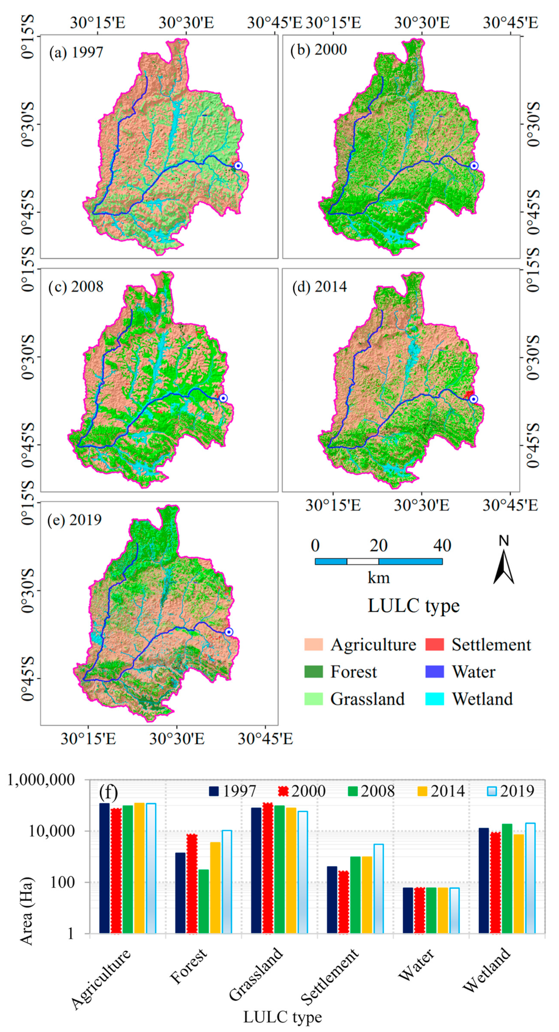
Figure 3.
Monthly rainfall based on observed and (a) CFSR, (b) CenTrends, (c) CRU, (d) CHIRPS, and (e) JRA55 data.
Figure 3.
Monthly rainfall based on observed and (a) CFSR, (b) CenTrends, (c) CRU, (d) CHIRPS, and (e) JRA55 data.

Figure 4.
(a) Monthly time series and (b) scatter plots of observed and modeled flow.
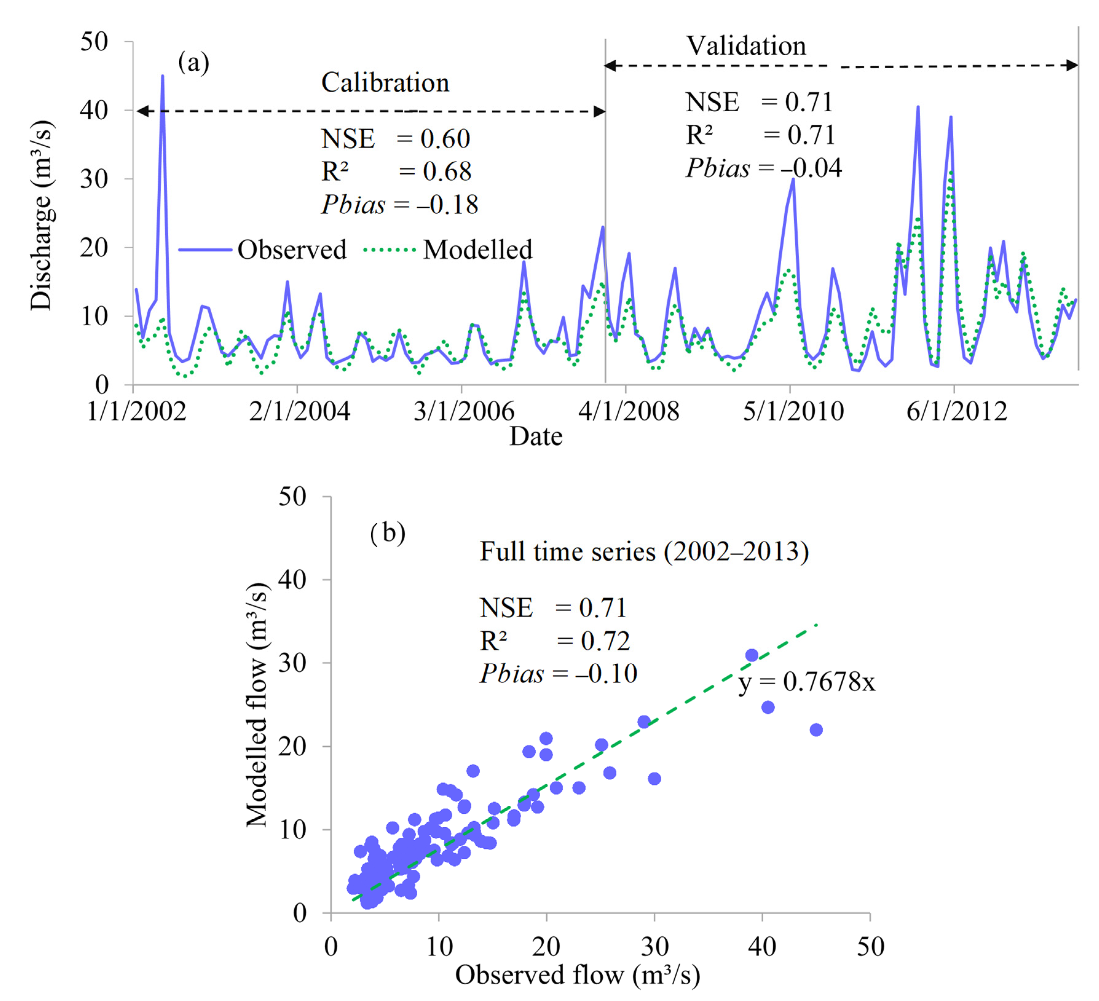
Figure 5.
Co-variation of rainfall, flow, and climate indices.
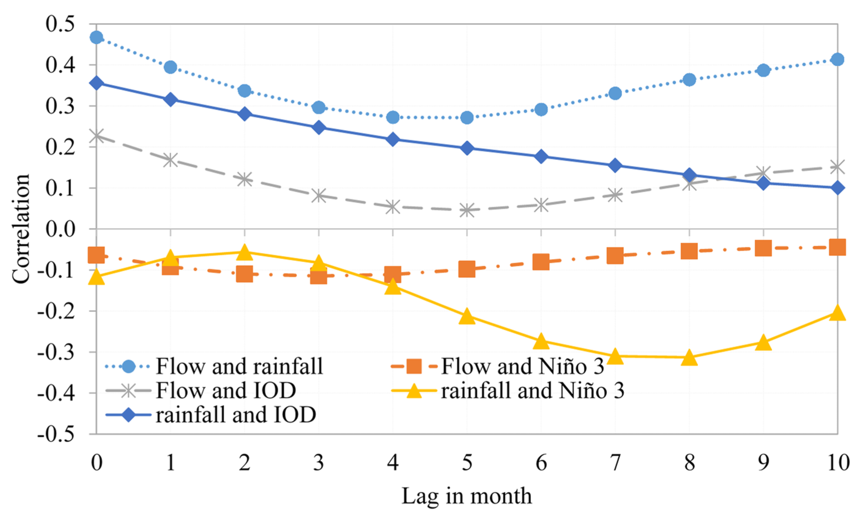
Figure 6.
Monthly (a) observed (Obs) and simulated river flow based on different LULC maps, and (b) catchment-wide averaged rainfall.
Figure 6.
Monthly (a) observed (Obs) and simulated river flow based on different LULC maps, and (b) catchment-wide averaged rainfall.
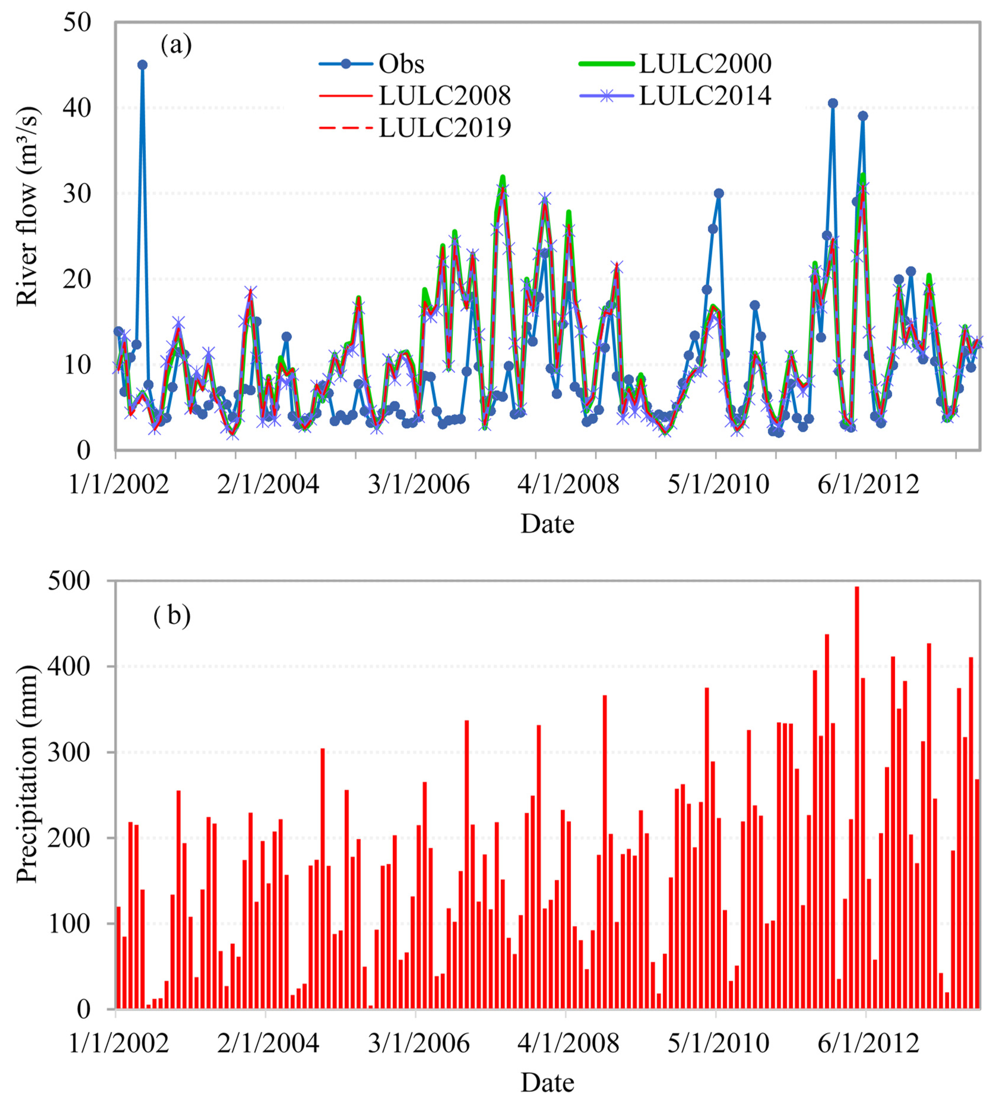
Figure 7.
Contribution of human impacts to monthly river flow variation.

Table 1.
Proportion of total catchment area under various LULC types.
| LULC | Area (%) | ||||
|---|---|---|---|---|---|
| 1997 | 2000 | 2008 | 2014 | 2019 | |
| Cropland | 38.2 | 23.0 | 39.1 | 51.6 | 31.6 |
| Forest | 1.7 | 3.7 | 1.3 | 3.7 | 9.8 |
| Grassland | 54.7 | 63.3 | 52.3 | 37.8 | 36.6 |
| Settlement | 0.1 | 0.1 | 0.4 | 0.4 | 4.8 |
| Water | 1.8 | 1.8 | 1.7 | 1.7 | 1.6 |
| Wetland | 3.5 | 8.1 | 5.2 | 4.7 | 15.6 |
Table 2.
LULC change summary for the River Rwizi catchment.
| LULC Type | Change in LULC Area (Ha) | |||
|---|---|---|---|---|
| 1997–2000 | 2000–2008 | 2008–2014 | 2014–2019 | |
| Cropland | −126,495 | 134,144 | 103,496 | −165,811 |
| Forest | 17,244 | −20,010 | 19,959 | 50,232 |
| Grassland | 71,322 | −91,235 | −120,202 | −10,468 |
| Settlement | −31 | 2222 | 266 | 35,939 |
| Water | −1034 | −3 | 709 | −533 |
| Wetland | 38,992 | −25,117 | −4229 | 90,641 |
Table 3.
Correlation between observed river flow and reanalysis or satellite rainfall.
| Data | Jan | Feb | March | April | May | June | July | Aug | Sept | Oct | Nov | Dec |
|---|---|---|---|---|---|---|---|---|---|---|---|---|
| No lag | ||||||||||||
| CFSR | 0.12 | 0.62 | 0.44 | 0.58 | 0.25 | 0.06 | −0.34 | 0.15 | 0.68 | 0.64 | 0.46 | 0.54 |
| CRU | −0.58 | −0.19 | −0.50 | −0.25 | −0.14 | −0.34 | −0.11 | 0.03 | −0.06 | 0.20 | 0.18 | 0.36 |
| CHIRPS | 0.23 | 0.45 | 0.61 | 0.31 | 0.60 | 0.33 | −0.13 | −0.15 | 0.76 | 0.18 | 0.27 | 0.22 |
| JRA55 | 0.01 | −0.06 | 0.16 | −0.08 | 0.25 | 0.04 | 0.00 | −0.22 | 0.35 | 0.26 | 0.01 | 0.00 |
| CenTrends | 0.14 | 0.48 | 0.38 | 0.50 | 0.16 | 0.51 | 0.15 | 0.18 | 0.30 | −0.13 | 0.24 | 0.29 |
| 1-month lag | ||||||||||||
| CFSR | 0.36 | 0.38 | −0.13 | 0.30 | −0.04 | 0.04 | −0.40 | 0.39 | 0.30 | 0.49 | 0.52 | −0.25 |
| CRU | −0.04 | −0.60 | −0.08 | −0.06 | −0.12 | −0.02 | −0.17 | −0.46 | −0.08 | 0.28 | 0.28 | −0.10 |
| CHIRPS | 0.11 | 0.44 | −0.47 | 0.13 | −0.22 | 0.28 | −0.68 | 0.34 | 0.20 | 0.21 | 0.26 | −0.31 |
| JRA55 | −0.24 | −0.15 | −0.20 | −0.13 | −0.04 | 0.26 | −0.41 | 0.14 | 0.23 | 0.10 | −0.35 | −0.33 |
| CenTrends | 0.22 | 0.35 | 0.09 | −0.23 | 0.27 | 0.37 | −0.06 | 0.70 | −0.05 | 0.07 | 0.08 | −0.38 |
| 2-month lag | ||||||||||||
| CFSR | 0.41 | 0.07 | −0.42 | 0.04 | −0.12 | −0.06 | −0.36 | 0.14 | 0.60 | 0.28 | −0.23 | −0.04 |
| CRU | −0.54 | 0.11 | −0.09 | 0.16 | 0.45 | 0.34 | −0.44 | −0.05 | −0.11 | 0.61 | −0.27 | 0.78 |
| CHIRPS | 0.42 | −0.30 | −0.42 | −0.04 | −0.10 | −0.37 | −0.34 | −0.34 | 0.34 | −0.12 | −0.14 | −0.07 |
| JRA55 | −0.14 | −0.03 | 0.15 | 0.03 | −0.17 | −0.46 | −0.36 | −0.13 | 0.11 | −0.65 | −0.25 | −0.11 |
| CenTrends | 0.21 | 0.22 | −0.03 | 0.55 | −0.22 | −0.27 | 0.15 | 0.09 | 0.10 | −0.15 | −0.28 | 0.06 |
| 3-month lag | ||||||||||||
| CFSR | 0.43 | −0.24 | −0.25 | −0.08 | −0.15 | 0.01 | −0.02 | 0.35 | 0.34 | −0.05 | 0.26 | 0.21 |
| CRU | 0.44 | 0.32 | −0.10 | 0.24 | 0.37 | 0.00 | 0.31 | 0.02 | 0.58 | −0.39 | 0.67 | 0.38 |
| CHIRPS | −0.02 | −0.47 | −0.08 | −0.24 | −0.42 | −0.21 | 0.14 | 0.39 | −0.14 | −0.16 | 0.16 | −0.56 |
| JRA55 | 0.14 | 0.04 | 0.25 | −0.37 | −0.35 | −0.23 | 0.25 | 0.21 | −0.35 | −0.22 | 0.18 | −0.22 |
| CenTrends | 0.40 | 0.04 | 0.10 | −0.16 | −0.47 | 0.01 | 0.56 | 0.13 | −0.03 | −0.34 | 0.26 | −0.26 |
Table 4.
Sensitivity rankings of river flow parameters in the River Rwizi catchment.
| S/N | Parameter Name | Description | t-Stat | p-Value |
|---|---|---|---|---|
| 1 | v__ALPHA_BF | Base flow alpha factor (days) | 10.49 | 2.53 × 10⁻²³ |
| 2 | v__HRU_SLP | Average slope steepness (m/m) | 6.43 | 3.00 × 10⁻¹⁰ |
| 3 | r__CN2 | Moisture condition II curve number | 5.11 | 4.49 × 10⁻⁷ |
| 4 | v__GWQMN | Threshold water level in shallow aquifer for base flow to occur (mm) | −4.49 | 9.00 × 10⁻⁶ |
| 5 | v__SOL_BD | Moist bulk density (g/cm3) | 4.074 | 5.40 × 10⁻⁵ |
| 6 | v__CH_K2 | Effective hydraulic conductivity of main channel alluvium (mm/hr) | −3.32 | 9.49 × 10⁻⁴ |
| 7 | v__SLSUBBSN | Average slope length (m) | −3.14 | 1.77 × 10⁻³ |
| 8 | r__SOL_AWC | Available water capacity of the soil layer (mm H2O/mm soil) | 2.48 | 1.34 × 10⁻² |
| 9 | v__REVAPMN | Threshold depth of water in the shallow aquifer for percolation to the deep aquifer to occur (mm. H2O). | 1.65 | 9.82 × 10⁻¹ |
| 10 | r__SOL_K | Saturated hydraulic conductivity (mm/h) | 1.62 | 1.06 × 10⁻¹ |
| 11 | v__ESCO | Plant uptake compensation factor | 1.41 | 1.60 × 10⁻¹ |
| 12 | r__GW_REVAP | Groundwater evapotranspiration coefficient | −1.24 | 2.13 × 10⁻¹ |
| 13 | v__CH_N2 | Manning’s “n” value for the main channel | −0.93 | 3.55 × 10⁻¹ |
v__ means to multiply by original value, and r__ means replace original value.
Publisher’s Note: MDPI stays neutral with regard to jurisdictional claims in published maps and institutional affiliations. |
© 2021 by the authors. Licensee MDPI, Basel, Switzerland. This article is an open access article distributed under the terms and conditions of the Creative Commons Attribution (CC BY) license (https://creativecommons.org/licenses/by/4.0/).
Share and Cite
MDPI and ACS Style
Onyutha, C.; Nyesigire, R.; Nakagiri, A. Contributions of Human Activities and Climatic Variability to Changes in River Rwizi Flows in Uganda, East Africa. Hydrology 2021, 8, 145. https://doi.org/10.3390/hydrology8040145
AMA Style
Onyutha C, Nyesigire R, Nakagiri A. Contributions of Human Activities and Climatic Variability to Changes in River Rwizi Flows in Uganda, East Africa. Hydrology. 2021; 8(4):145. https://doi.org/10.3390/hydrology8040145
Chicago/Turabian StyleOnyutha, Charles, Resty Nyesigire, and Anne Nakagiri. 2021. "Contributions of Human Activities and Climatic Variability to Changes in River Rwizi Flows in Uganda, East Africa" Hydrology 8, no. 4: 145. https://doi.org/10.3390/hydrology8040145
Note that from the first issue of 2016, this journal uses article numbers instead of page numbers. See further details here.