Characterization of Temporal and Spatial Variability of Phosphorus Loading to Lake Erie from the Western Basin Using Wavelet Transform Methods

Abstract
:1. Introduction
2. Theoretical Background
2.1. Wavelet Analysis
2.2. Continuous Wavelet Transform (CWT)
2.3. Discrete Wavelet Transform (DWT)
3. Methodology
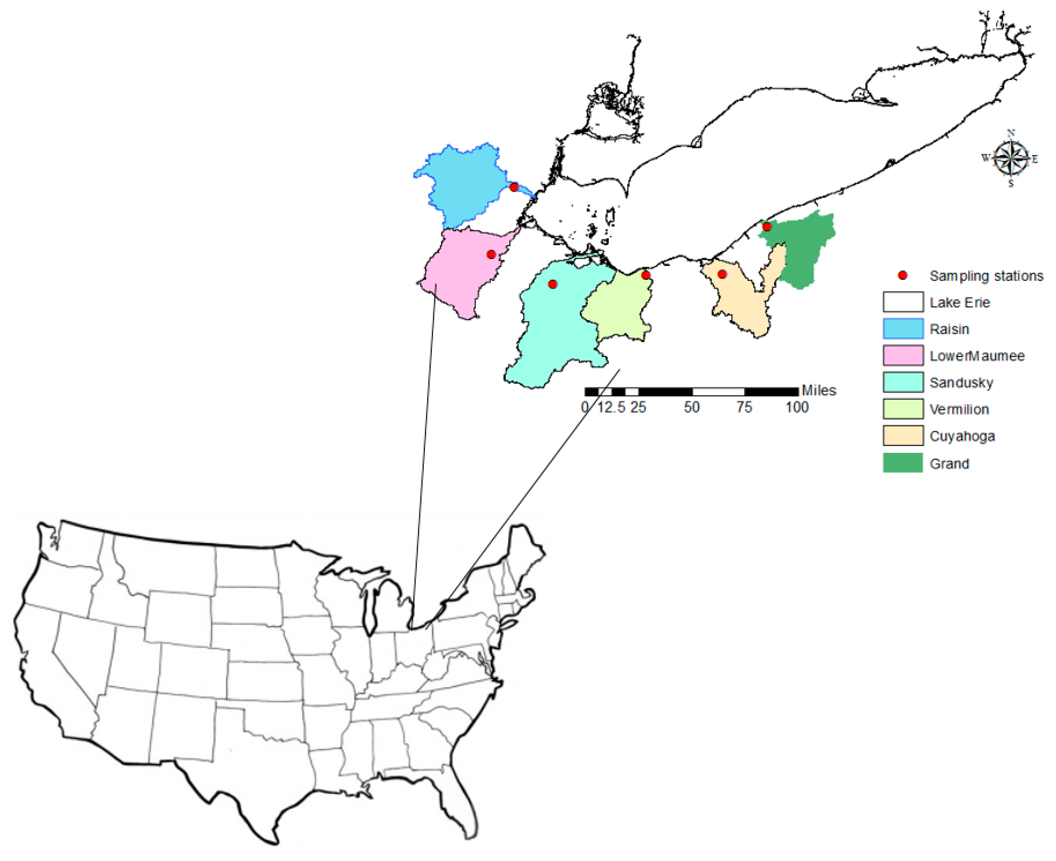
4. Study Area
4.1. Continuous Wavelet Transform
4.2. Discrete Wavelet Transform
5. Results and Discussion
5.1. Wavelet Analysis
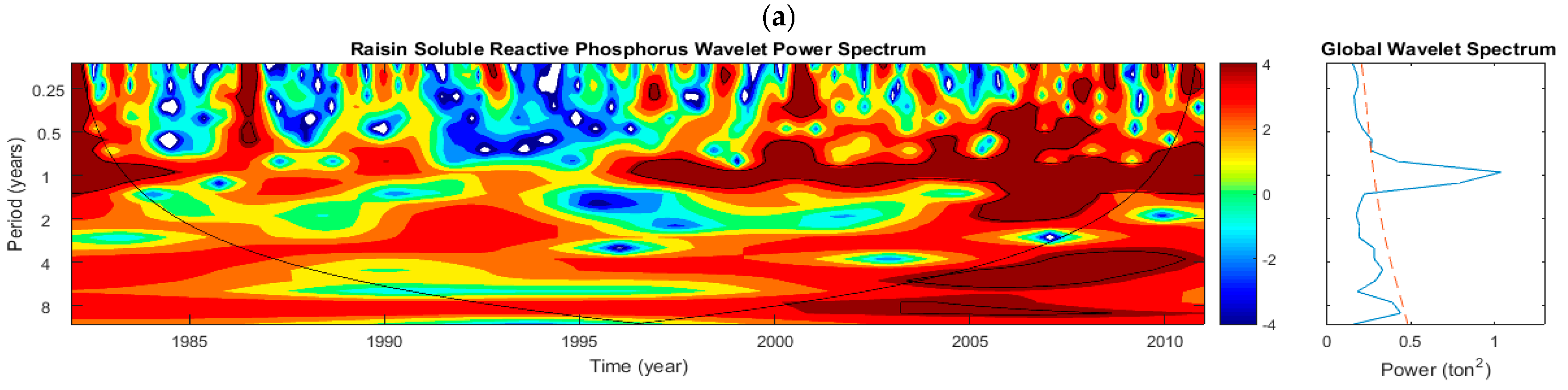
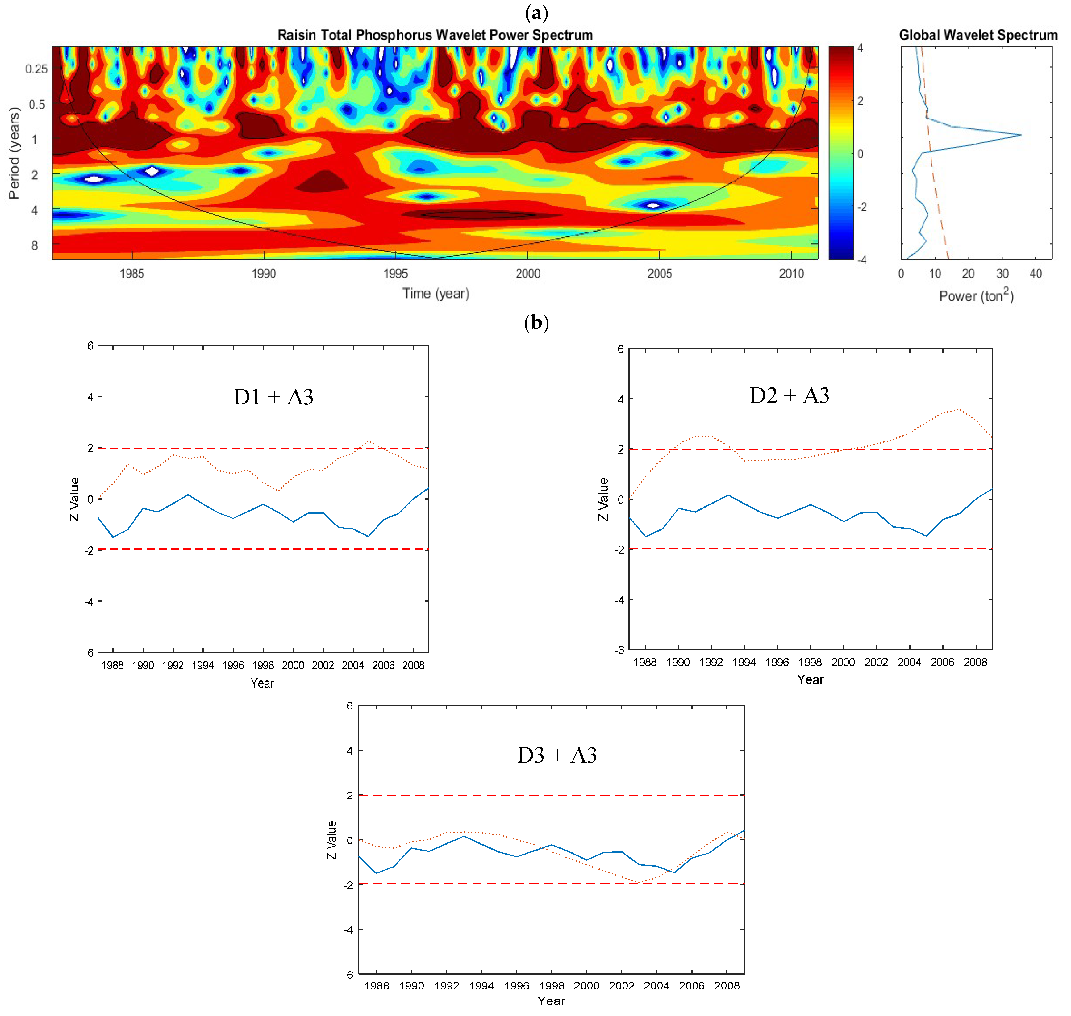
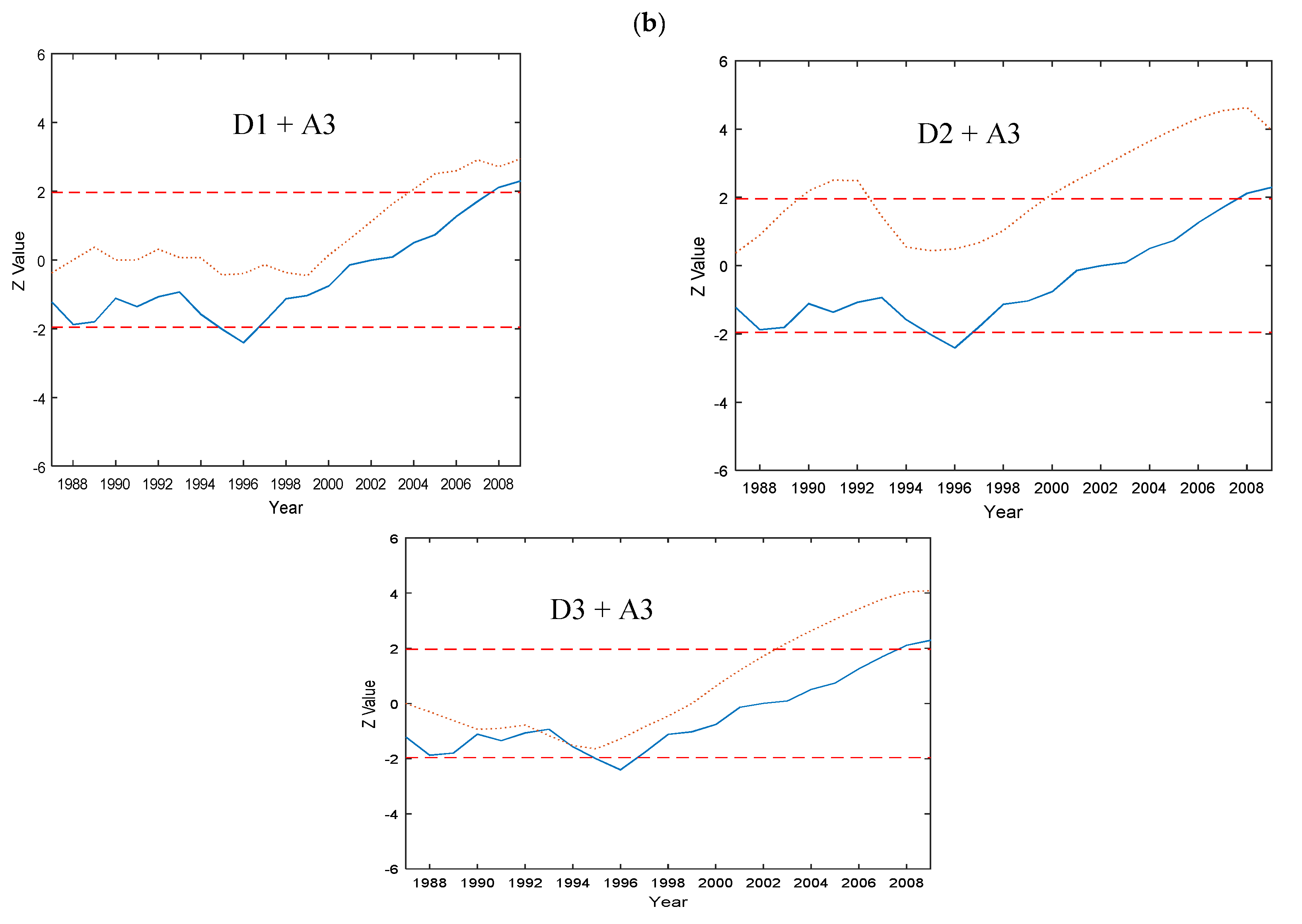
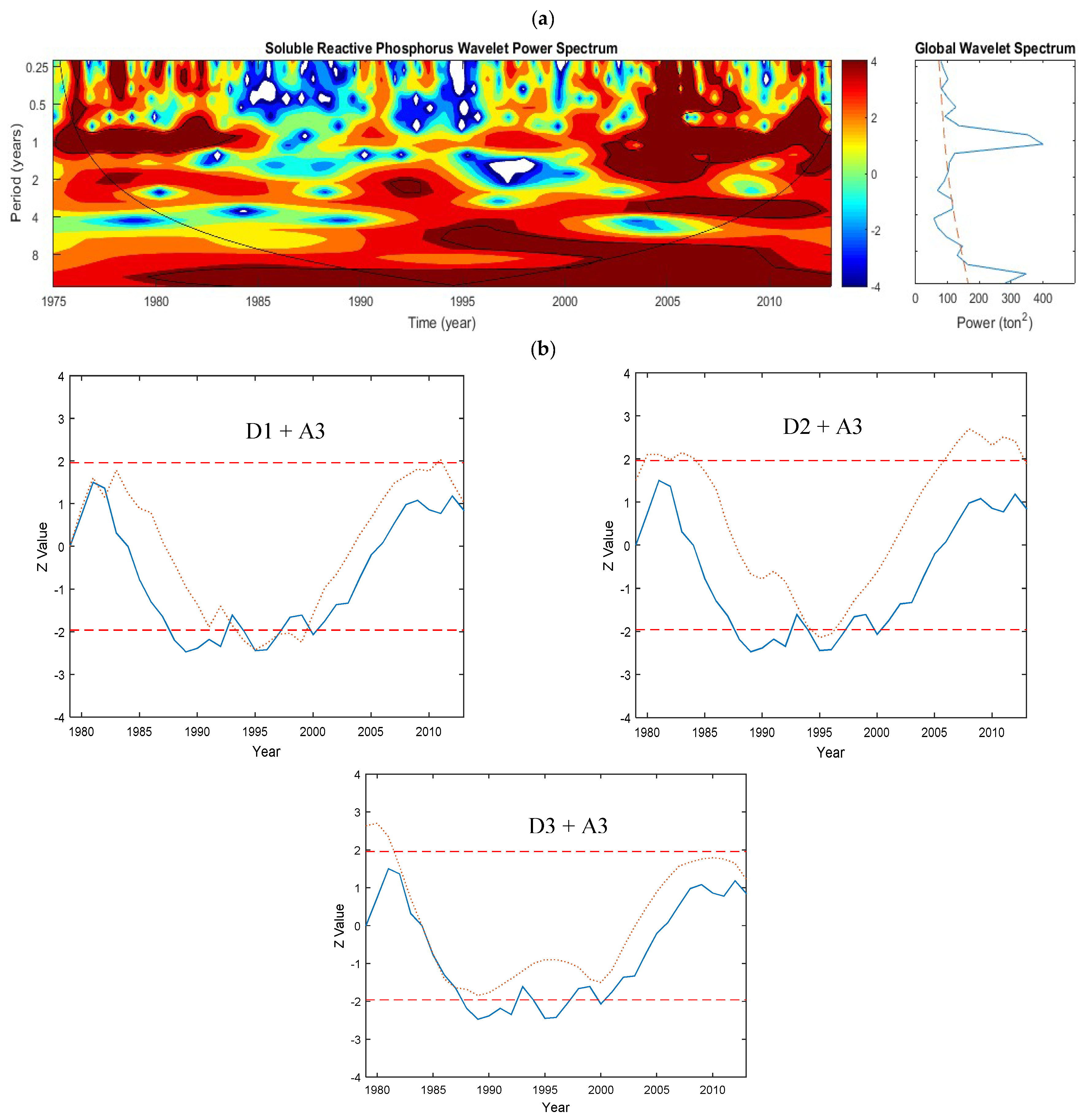
5.1.1. Raisin Watershed—Phosphorus
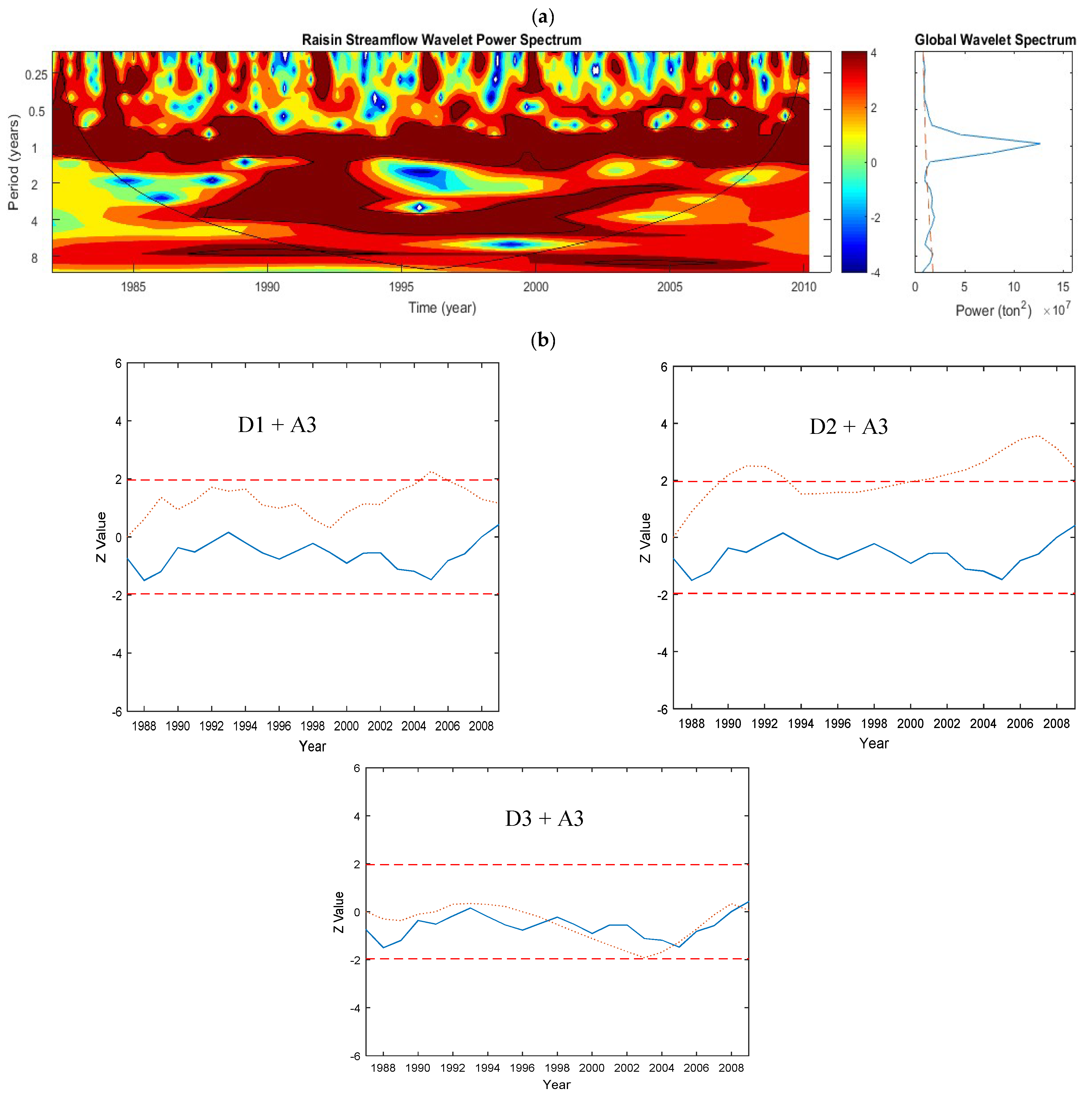
5.1.2. Raisin Watershed—Flow
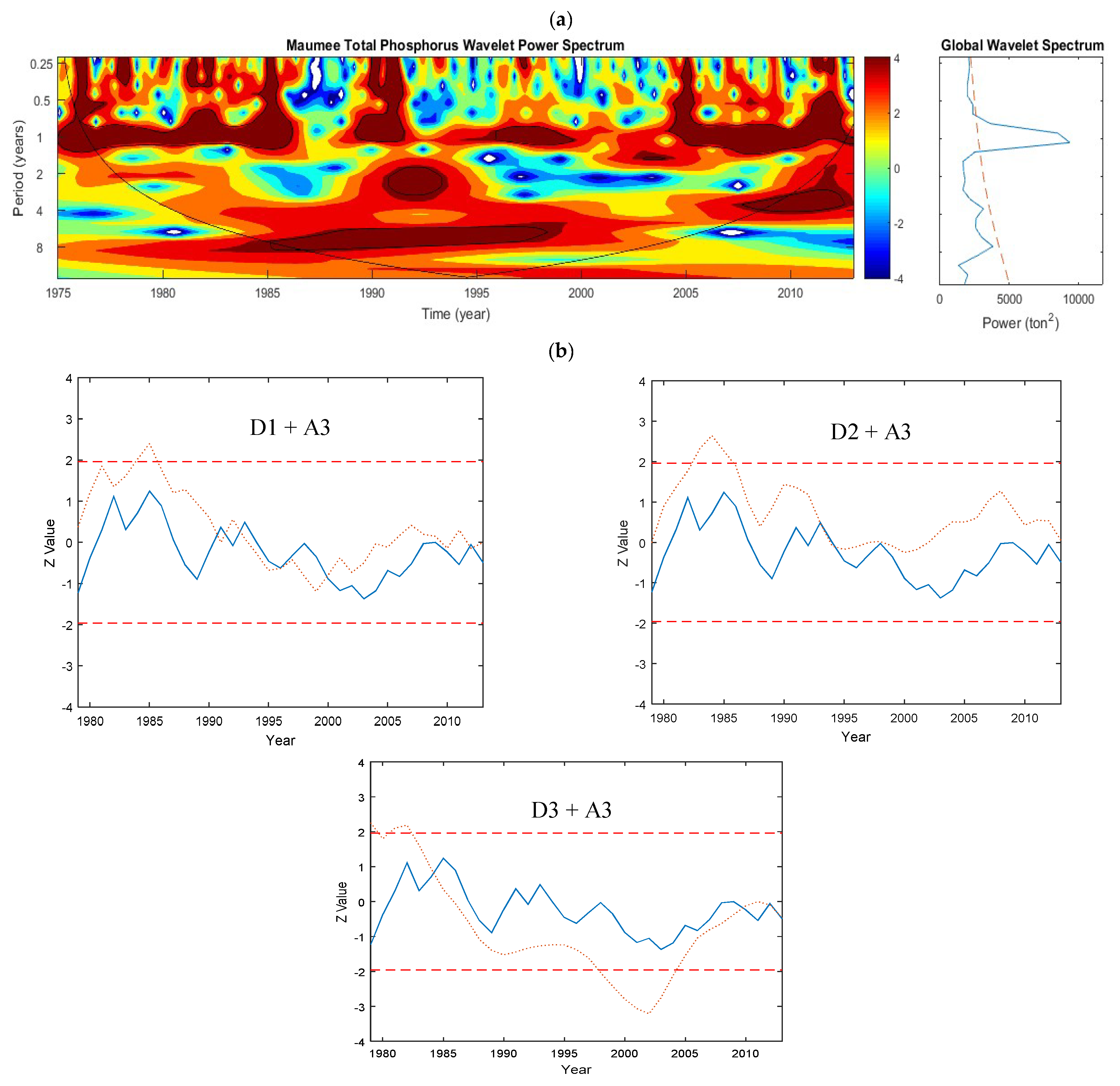
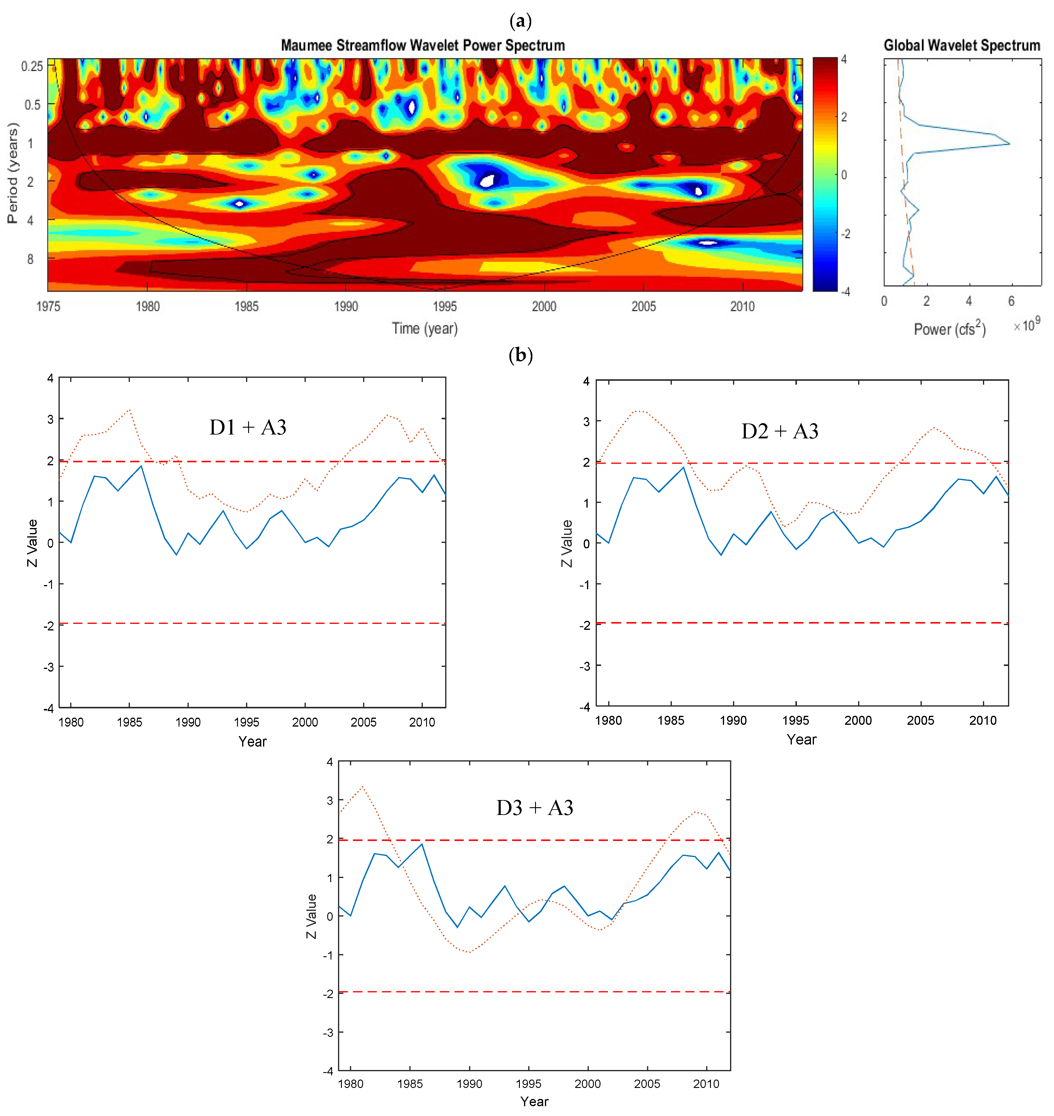
5.1.3. Maumee Watershed—Phosphorus
5.1.4. Maumee Watershed—Flow
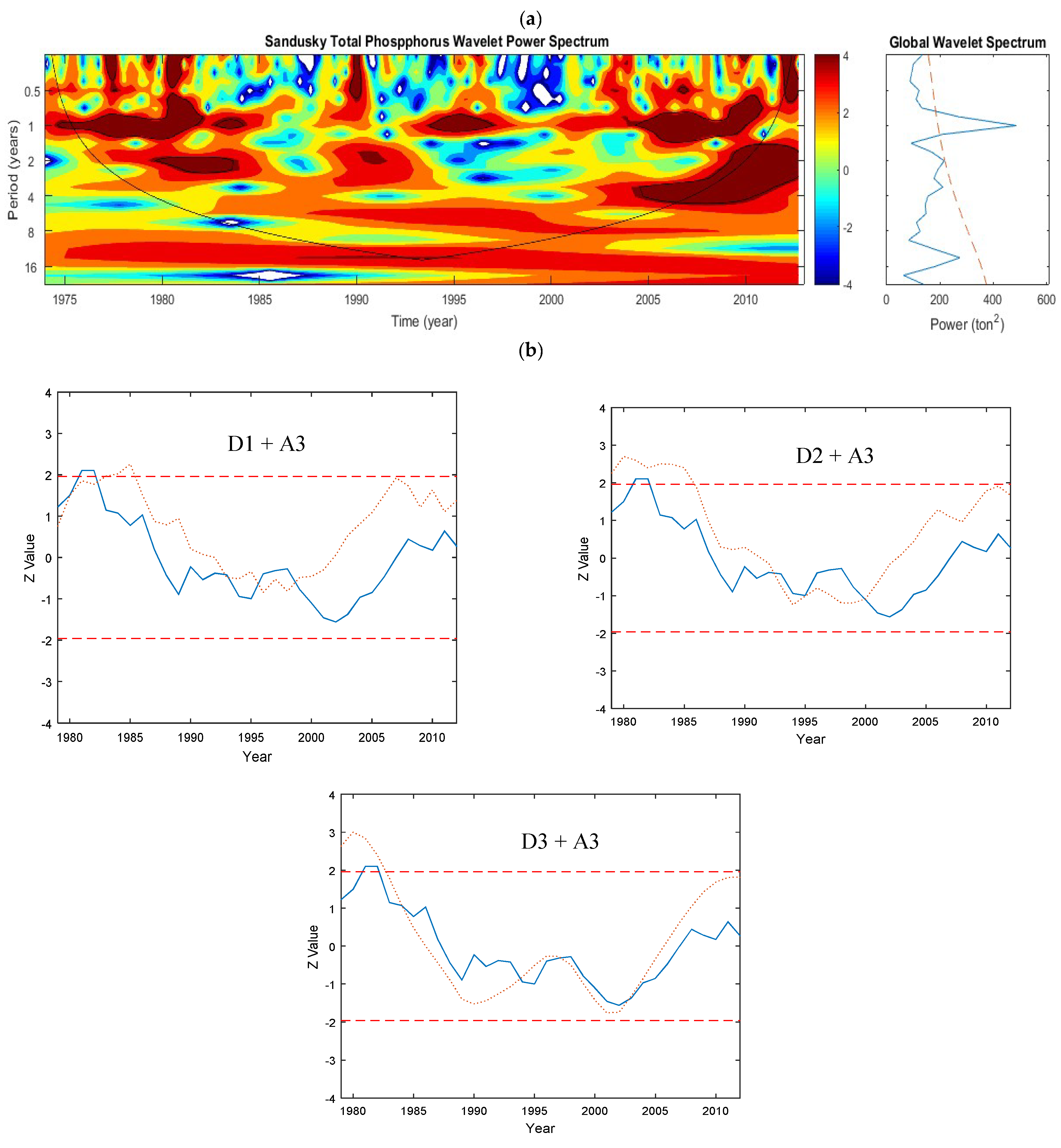
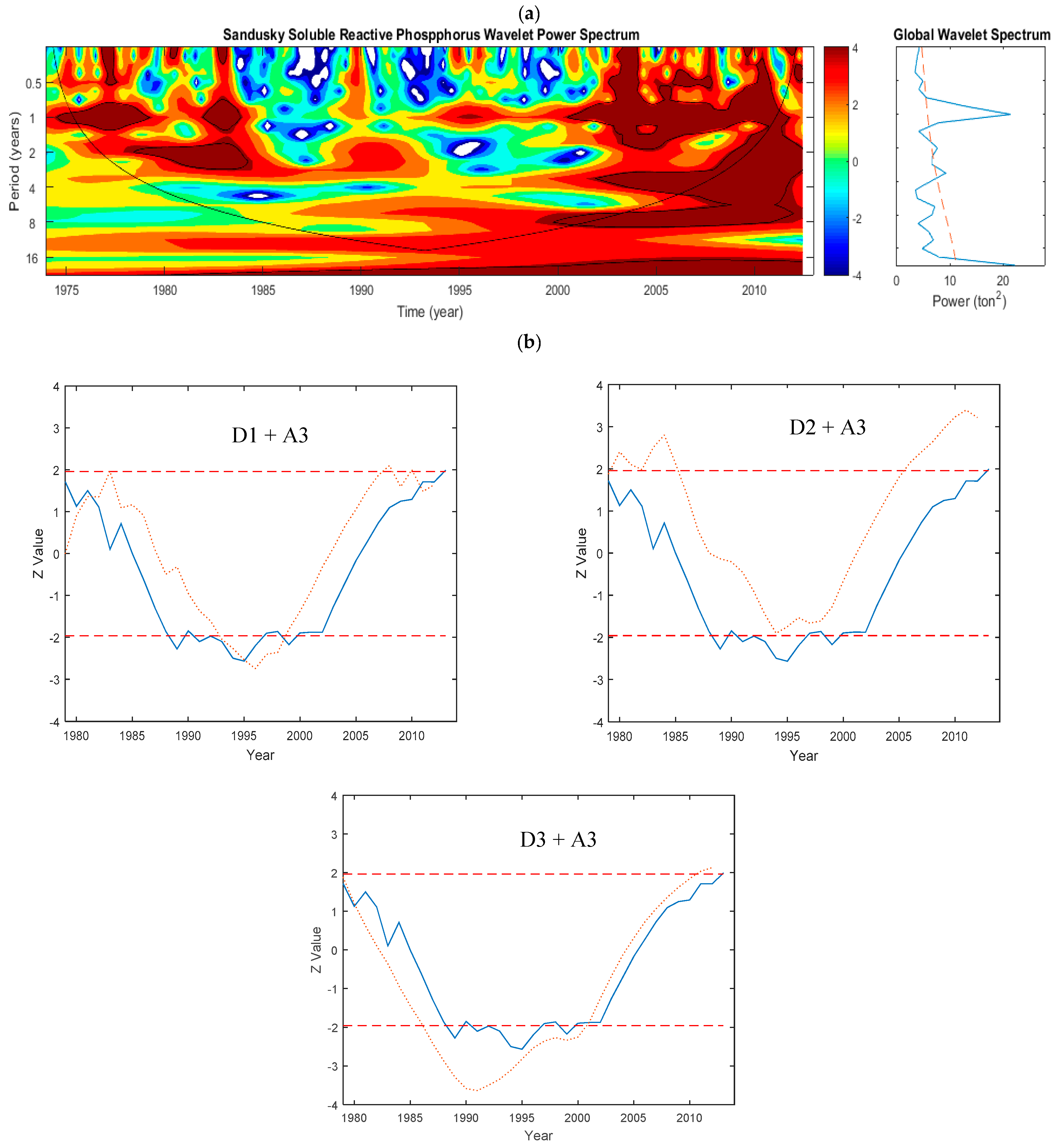
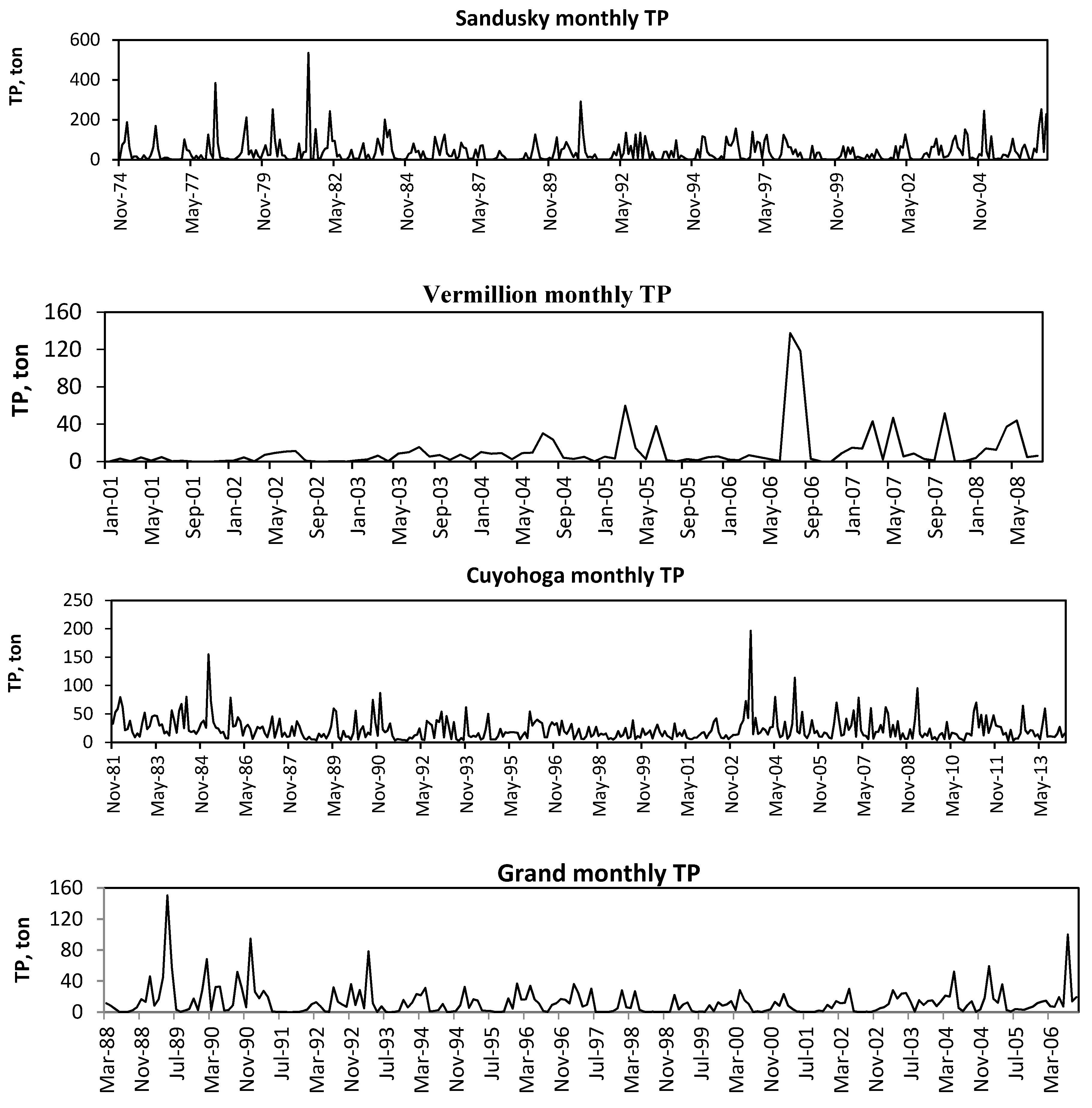
5.1.5. Sandusky Watershed—Phosphorus
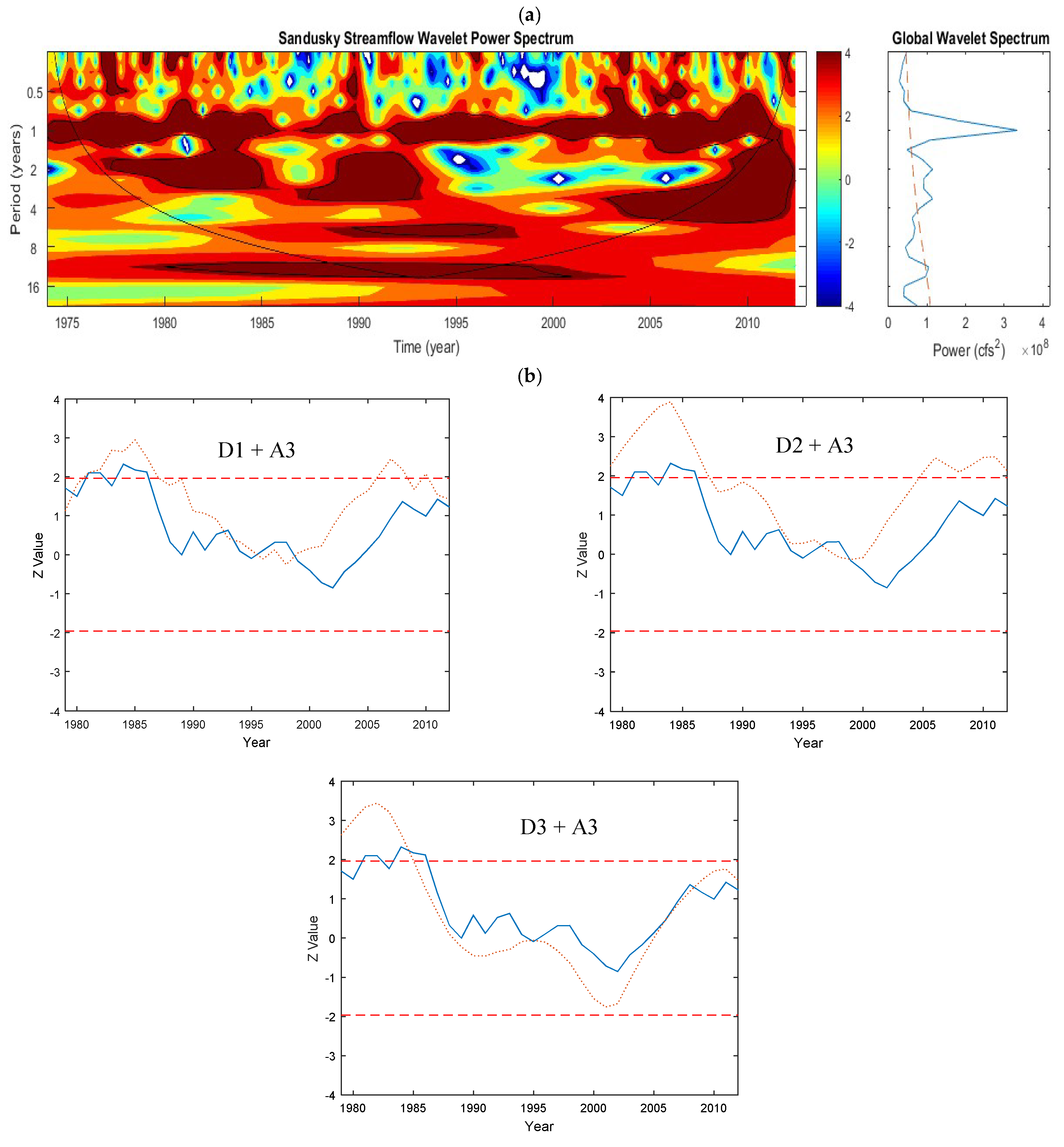
5.1.6. Sandusky Watershed—Flow
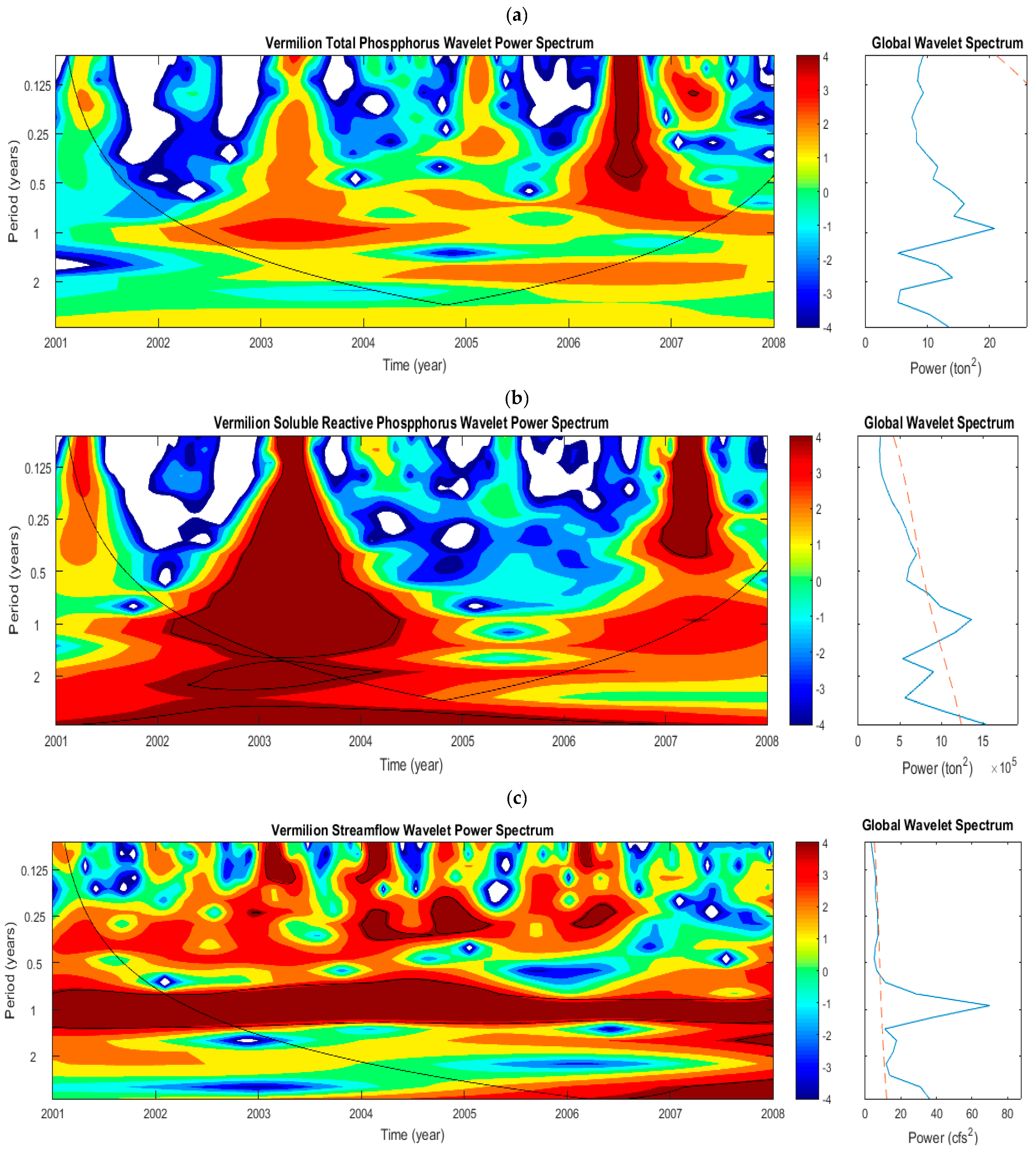
5.1.7. Vermilion Watershed—Phosphorus
5.1.8. Vermilion Watershed—Flow
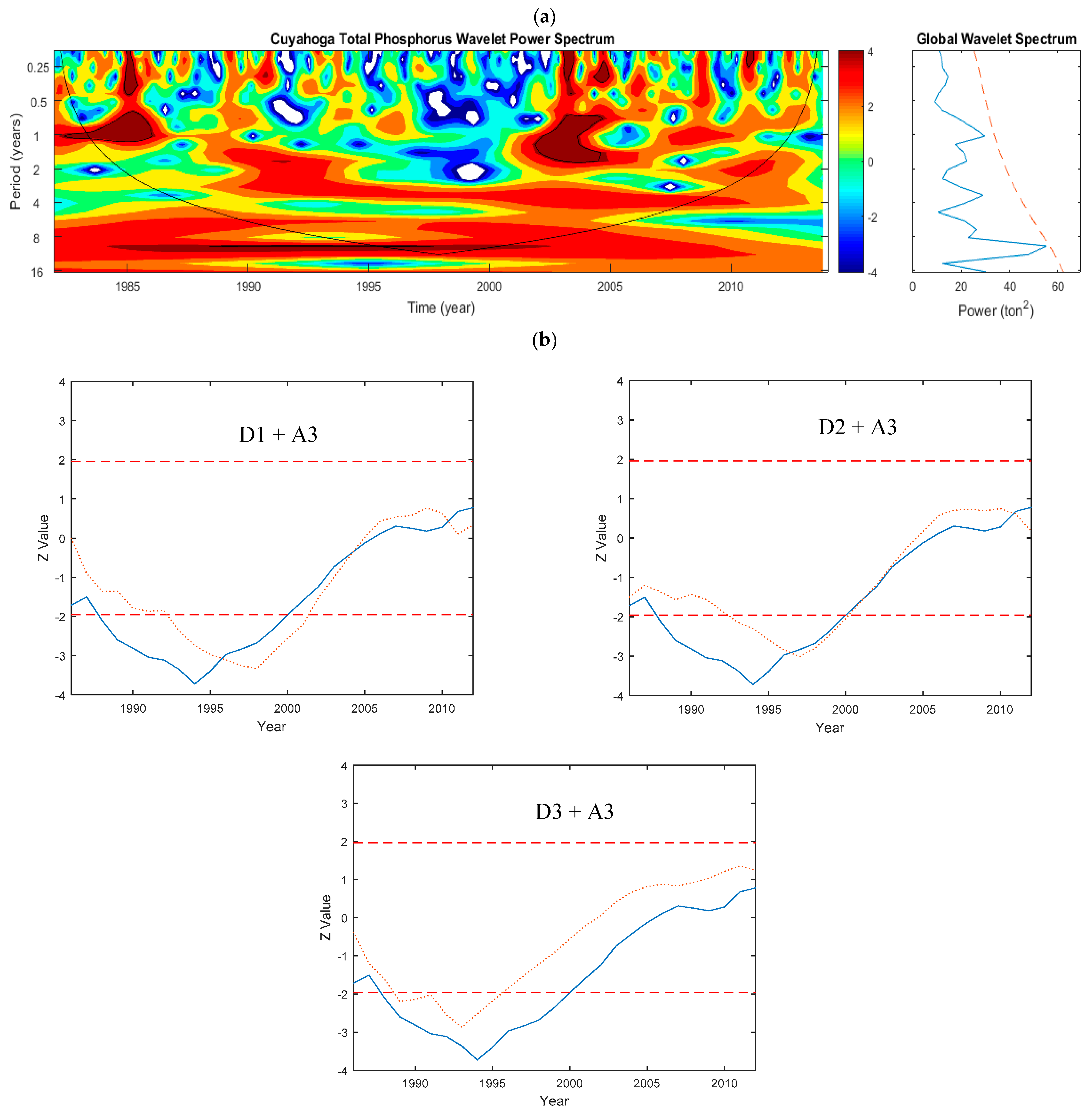
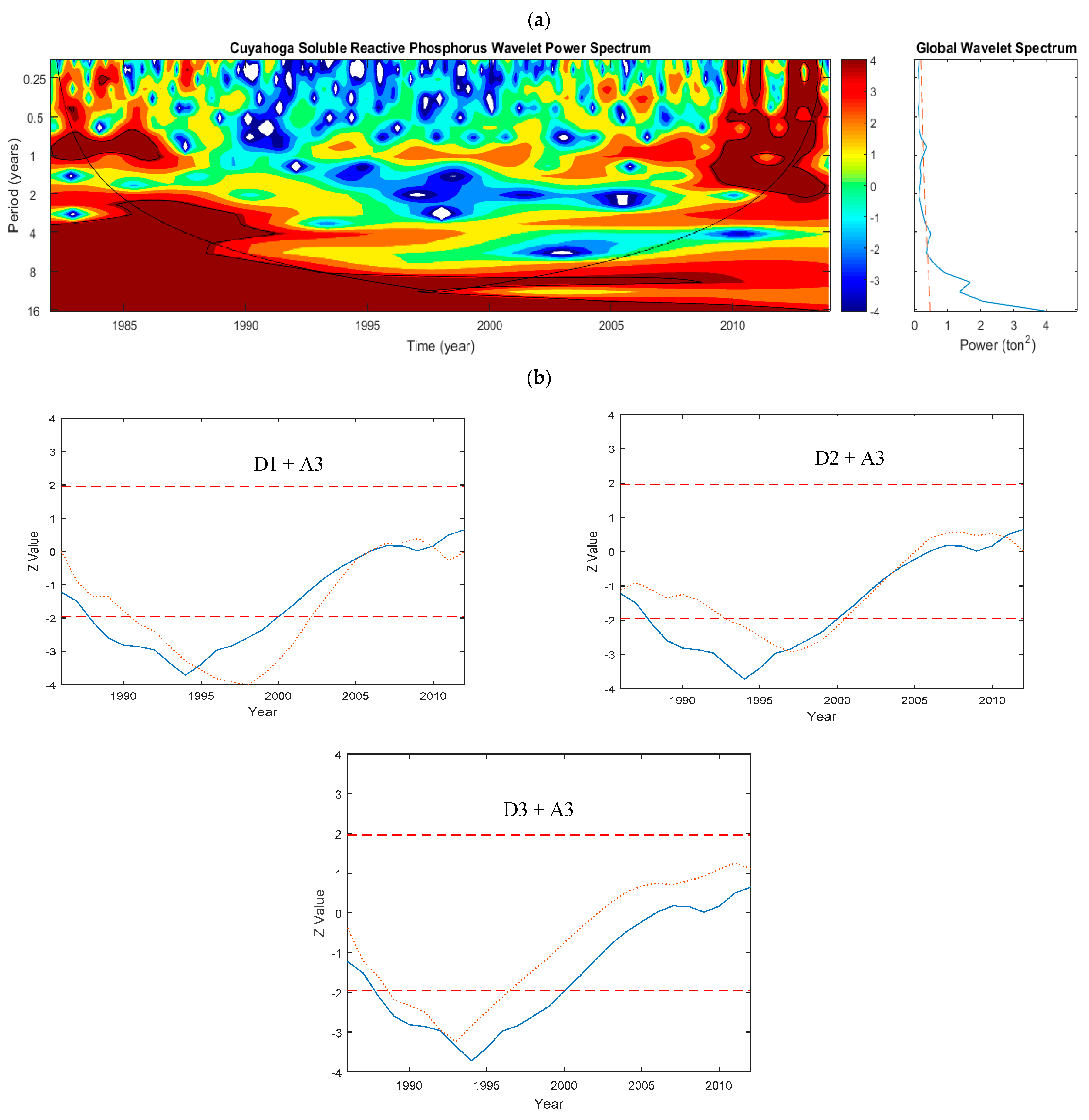
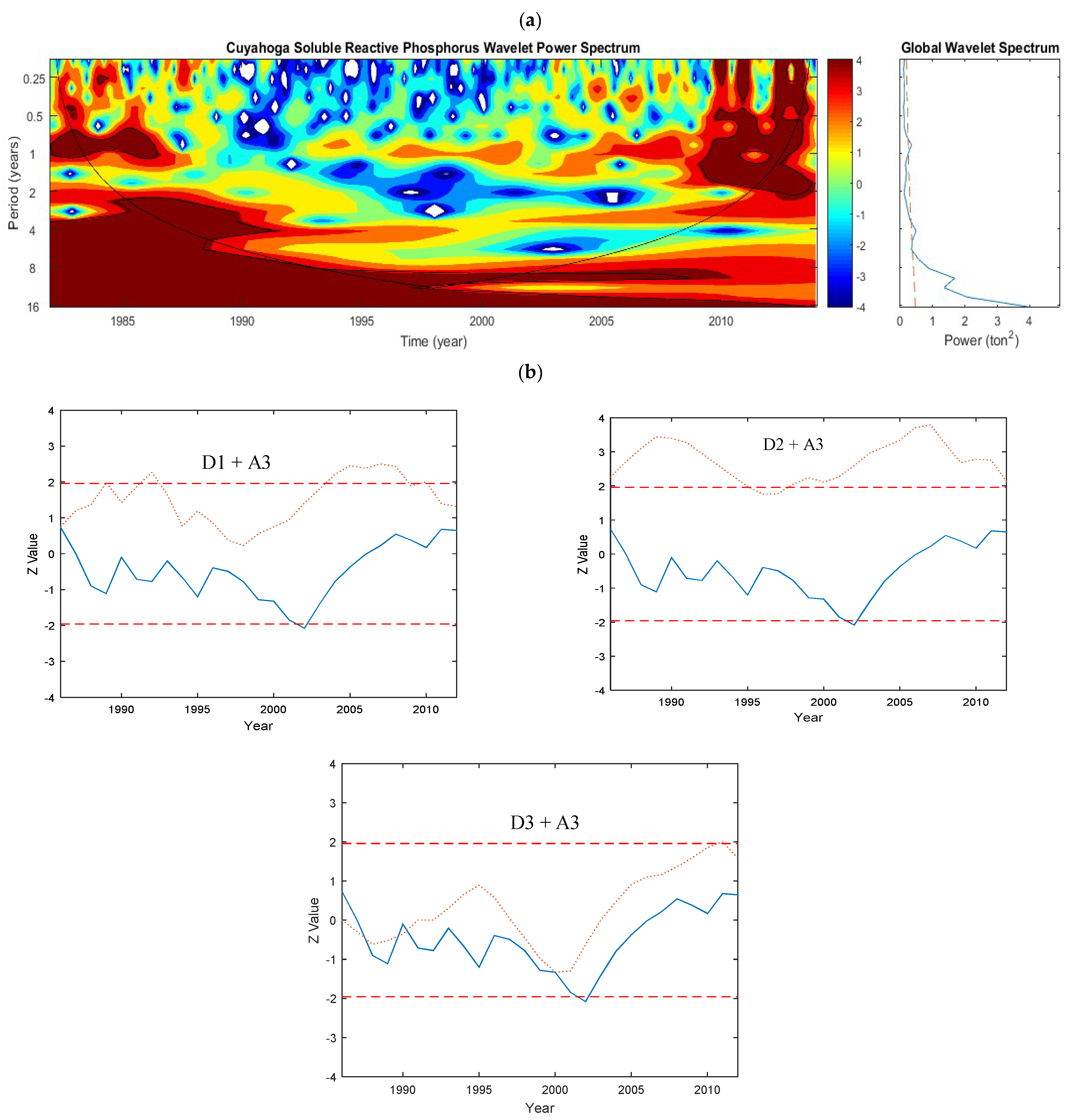
5.1.9. Cuyahoga Watershed—Phosphorus
5.1.10. Cuyahoga Watershed—Flow
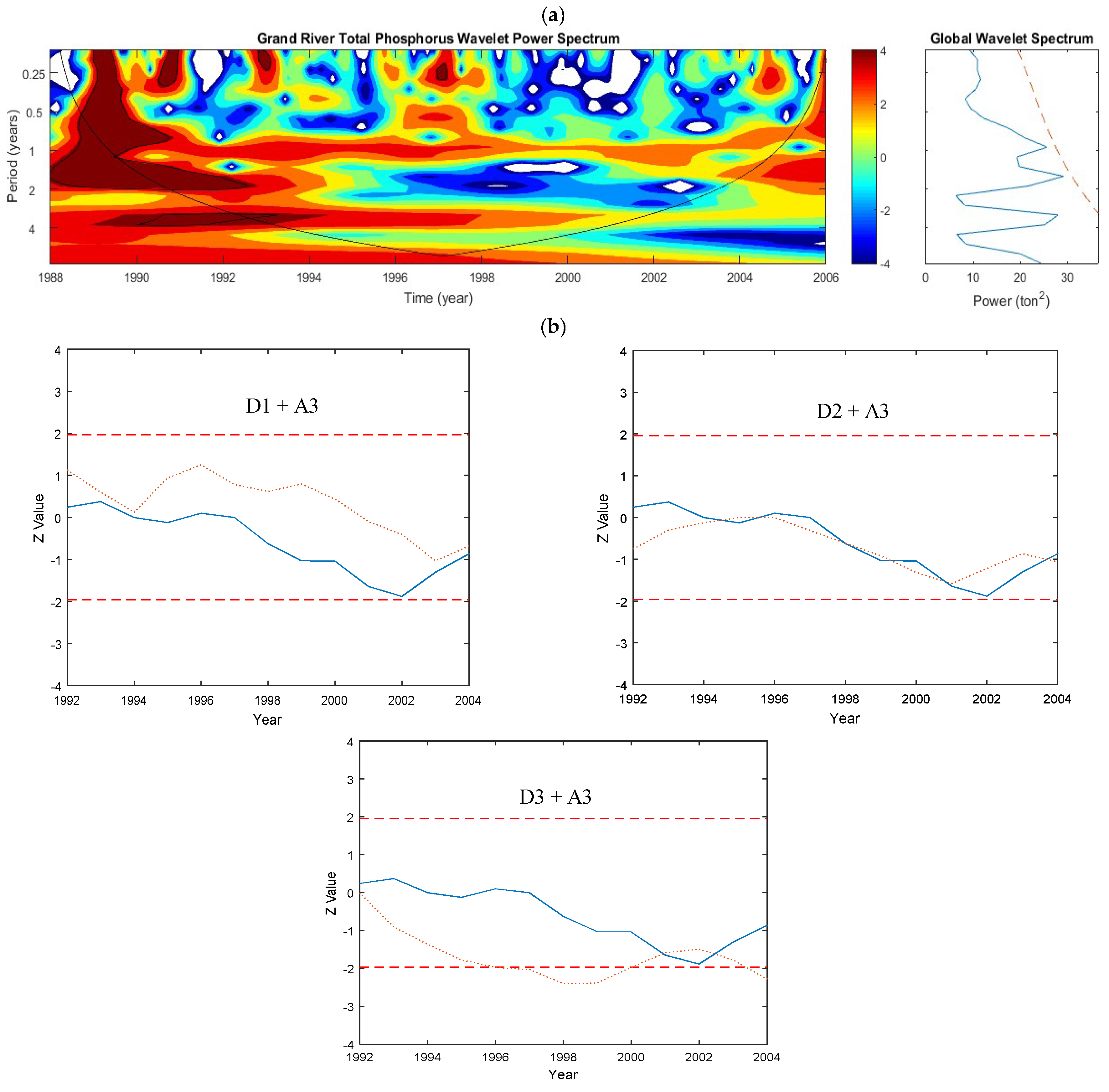
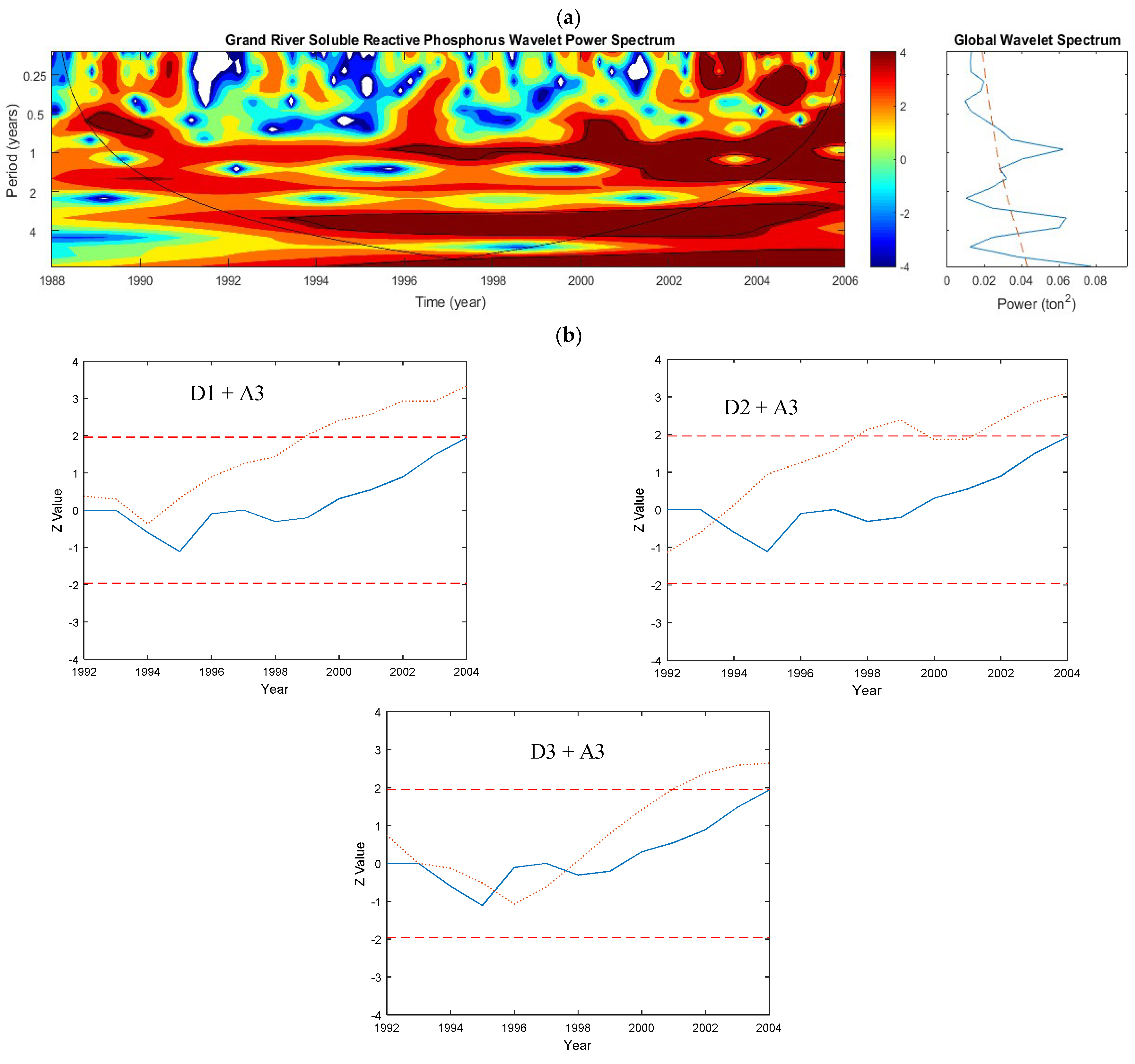
5.1.11. Grand Watershed—Phosphorus
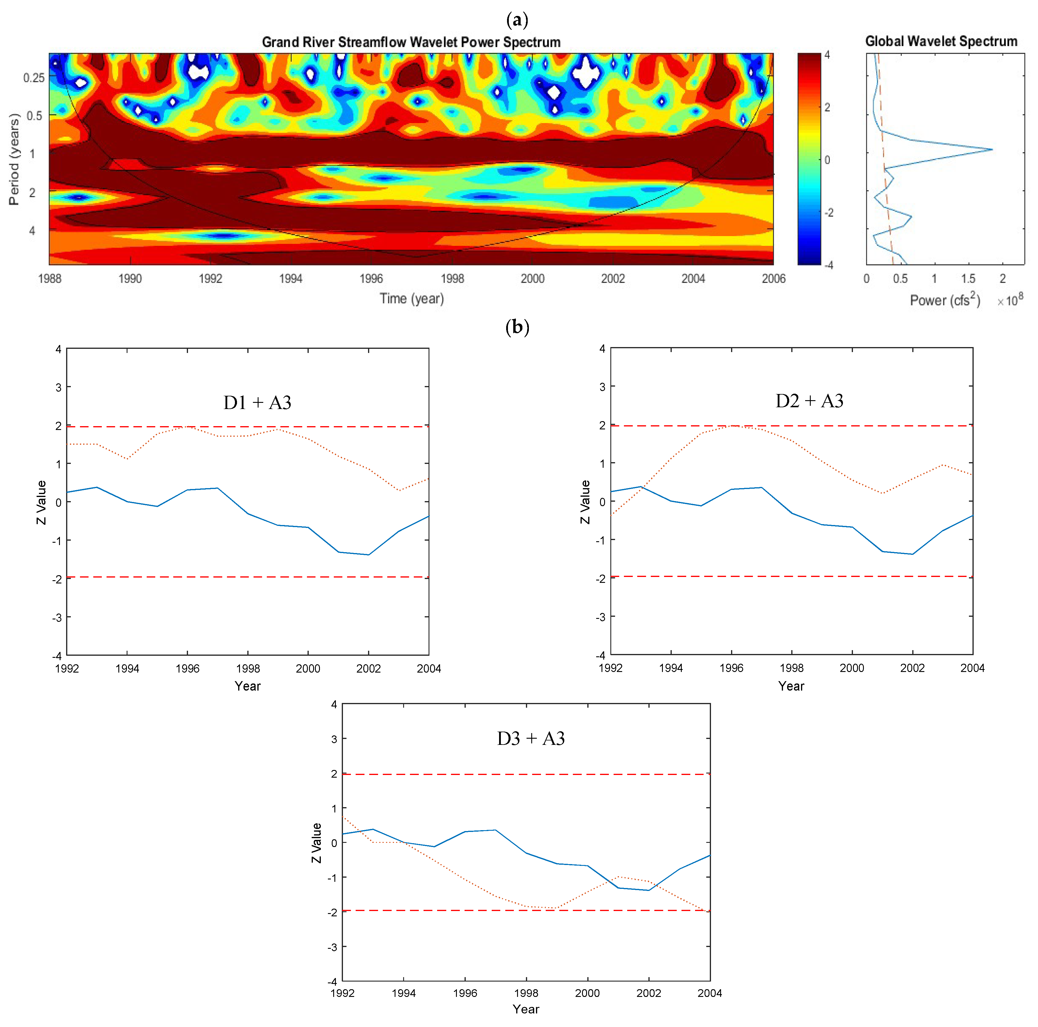
5.1.12. Grand Watershed—Flow
6. Summary and Conclusions
- The annual periodicity was highly significant and it contains the largest proportion of the variance of the time series. However, the variance varied considerably among the different sites.
- In addition to the annual periodicity, significant periodicities at higher scales were also revealed especially when long-term data were used. For the Maumee River, the 2-year and 8-year periodicities were also significant and, for the Sandusky River, the 2-year periodicity was significant. Periodicity of 2 and 8 year for Maumee River indicated the significant loading from Maumee River.
- The annual pattern of P loading was continuously significant for most sites. However, it was not significant in Grand and Cuyahoga Rivers.
Author Contributions
Funding
Conflicts of Interest
References
- Forster, D.L.; Richards, R.P.; Baker, D.B.; Blue, E.N. EPIC modeling of the effects of farming practice changes on water quality in two Lake Erie watersheds. J. Soil Water Conserv. 2000, 55, 85–90. [Google Scholar]
- Strickland, T.; Fisher, L.; Korleski, C. Ohio Lake Erie Phosphorus Task Force Final Report; Ohio Environmental Protection Agency, Division of Surface Water: Columbus, OH, USA, 2010.
- Dolan, D.M. Point source loadings of phosphorus to Lake Erie: 1986–1990. J. Great Lakes Res. 1993, 19, 212–223. [Google Scholar] [CrossRef]
- Dolan, D.M.; McGunagle, K.P. Lake Erie total phosphorus loading analysis and update: 1996–2002. J. Great Lakes Res. 2005, 31, 11–22. [Google Scholar] [CrossRef]
- Vanderploeg, H.A.; Nalepa, T.F.; Jude, D.J.; Mills, E.L.; Holeck, K.T.; Liebig, J.R.; Grigorovich, I.A.; Ojaveer, H. Dispersal and emerging ecological impacts of Ponto-Caspian species in the Laurentian Great Lakes. Can. J. Fish. Aquat. Sci. 2002, 59, 1209–1228. [Google Scholar] [CrossRef]
- Conroy, J.D.; Edwards, W.J.; Pontius, R.A.; Kane, D.D.; Zhang, H.; Shea, J.F.; Richey, J.N.; Culver, D.A. Soluble nitrogen and phosphorus excretion of exotic freshwater mussels (Dreissena spp.): Potential impacts for nutrient remineralisation in western Lake Erie. Freshw. Biol. 2005, 50, 1146–1162. [Google Scholar] [CrossRef]
- Bertram, P.E. Total phosphorus and dissolved oxygen trends in the central basin of Lake Erie, 1970–1991. J. Great Lakes Res. 1993, 19, 224–236. [Google Scholar] [CrossRef]
- Makarewicz, J.C.; Bertram, P. Evidence for the restoration of the Lake Erie ecosystem. Bioscience 1991, 41, 216–223. [Google Scholar] [CrossRef]
- Rosa, F.; Burns, N.M. Lake Erie central basin oxygen depletion changes from 1929–1980. J. Great Lakes Res. 1987, 13, 684–696. [Google Scholar] [CrossRef]
- De Pinto, J.V.; Young, T.C.; McIlroy, L.M. Great Lakes water quality improvement. Environ. Sci. Technol. 1986, 20, 752–759. [Google Scholar] [CrossRef] [PubMed]
- Bosch, N.S.; Evans, M.A.; Scavia, D.; Allan, J.D. Interacting effects of climate change and agricultural BMPs on nutrient runoff entering Lake Erie. J. Great Lakes Res. 2014, 40, 581–589. [Google Scholar] [CrossRef]
- Scavia, D.; Allan, J.D.; Arend, K.K.; Bartell, S.; Beletsky, D.; Bosch, N.S.; Brandt, S.B.; Briland, R.D.; Daloğlu, I.; DePinto, J.V. Assessing and addressing the re-eutrophication of Lake Erie: Central basin hypoxia. J. Great Lakes Res. 2014, 40, 226–246. [Google Scholar] [CrossRef]
- Ludsin, S.A.; Kershner, M.W.; Blocksom, K.A.; Knight, R.L.; Stein, R.A. Life after death in Lake Erie: Nutrient controls drive fish species richness, rehabilitation. Ecol. Appl. 2001, 11, 731–746. [Google Scholar] [CrossRef]
- Shea, M.A.; Makarewicz, J.C. Production, biomass, and trophic interactions of Mysis relicta in Lake Ontario. J. Great Lakes Res. 1989, 15, 223–232. [Google Scholar] [CrossRef]
- Charlton, M.N.; Milne, J.E.; Booth, W.G.; Chiocchio, F. Lake Erie offshore in 1990: Restoration and resilience in the central basin. J. Great Lakes Res. 1993, 19, 291–309. [Google Scholar] [CrossRef]
- Murphy, T.P.; Irvine, K.; Guo, J.; Davies, J.; Murkin, H.; Charlton, M.; Watson, S.B. New microcystin concerns in the lower Great Lakes. Water Qual. Res. J. Can. 2003, 38, 127–140. [Google Scholar] [CrossRef]
- Michalak, A.M.; Anderson, E.J.; Beletsky, D.; Boland, S.; Bosch, N.S.; Bridgeman, T.B.; Chaffin, J.D.; Cho, K.; Confesor, R.; Daloğlu, I. Record-setting algal bloom in Lake Erie caused by agricultural and meteorological trends consistent with expected future conditions. Proc. Natl. Acad. Sci. USA 2013, 110, 6448–6452. [Google Scholar] [CrossRef] [PubMed] [Green Version]
- Stumpf, R.P.; Wynne, T.T.; Baker, D.B.; Fahnenstiel, G.L. Interannual variability of cyanobacterial blooms in Lake Erie. PLoS ONE 2012, 7, e42444. [Google Scholar] [CrossRef] [PubMed]
- Pinto, M.R.; De Santis, R.; D’alessio, G.; Rosati, F. Studies on fertilization in the ascidians: Fucosyl sites on vitelline coat of Ciona intestinalis. Exp. Cell Res. 1981, 132, 289–295. [Google Scholar] [CrossRef]
- Richards, R.; Baker, D.; Crumrine, J.; Stearns, A. Unusually large loads in 2007 from the Maumee and Sandusky Rivers, tributaries to Lake Erie. J. Soil Water Conserv. 2010, 65, 450–462. [Google Scholar] [CrossRef] [Green Version]
- Vanderploeg, H.A.; Ludsin, S.A.; Ruberg, S.A.; Höök, T.O.; Pothoven, S.A.; Brandt, S.B.; Lang, G.A.; Liebig, J.R.; Cavaletto, J.F. Hypoxia affects spatial distributions and overlap of pelagic fish, zooplankton, and phytoplankton in Lake Erie. J. Exp. Mar. Biol. Ecol. 2009, 381, S92–S107. [Google Scholar] [CrossRef]
- Burns, N.M.; Rockwell, D.C.; Bertram, P.E.; Dolan, D.M.; Ciborowski, J.J. Trends in temperature, Secchi depth, and dissolved oxygen depletion rates in the central basin of Lake Erie, 1983–2002. J. Great Lakes Res. 2005, 31, 35–49. [Google Scholar] [CrossRef]
- Grimberg, A.; Coleman, C.M.; Burns, T.F.; Himelstein, B.P.; Koch, C.J.; Cohen, P.; El-Deiry, W.S. p53-Dependent and p53-independent induction of insulin-like growth factor binding protein-3 by deoxyribonucleic acid damage and hypoxia. J. Clin. Endocrinol. Metab. 2005, 90, 3568–3574. [Google Scholar] [CrossRef] [PubMed]
- Rucinski, D.K.; Beletsky, D.; DePinto, J.V.; Schwab, D.J.; Scavia, D. A simple 1-dimensional, climate based dissolved oxygen model for the central basin of Lake Erie. J. Great Lakes Res. 2010, 36, 465–476. [Google Scholar] [CrossRef]
- Bridgeman, T.B.; Penamon, W.A. Lyngbya wollei in western Lake Erie. J. Great Lakes Res. 2010, 36, 167–171. [Google Scholar] [CrossRef]
- Smith, D.R.; Francesconi, W.; Livingston, S.J.; Huang, C.-H. Phosphorus losses from monitored fields with conservation practices in the Lake Erie Basin, USA. Ambio 2015, 44, 319–331. [Google Scholar] [CrossRef] [PubMed] [Green Version]
- Richards, R.P. Trends in sediment and nutrients in major Lake Erie tributaries, 1975–2004. Lake Erie Lakewide Manag. Plan. 2006, 22. [Google Scholar]
- Yuan, H.; Liu, T.; Szarkowski, R.; Rios, C.; Ashe, J.; He, B. Negative covariation between task-related responses in alpha/beta-band activity and BOLD in human sensorimotor cortex: An EEG and FMRI study of motor imagery and movements. Neuroimage 2010, 49, 2596–2606. [Google Scholar] [CrossRef] [PubMed]
- Cazelles, B.; Chavez, M.; Berteaux, D.; Ménard, F.; Vik, J.O.; Jenouvrier, S.; Stenseth, N.C. Wavelet analysis of ecological time series. Oecologia 2008, 156, 287–304. [Google Scholar] [CrossRef] [PubMed]
- Sharma, S.; Srivastava, P. Teleconnection of Instream Total Organic Carbon Loads with El Niño Southern Oscillation (ENSO), North Atlantic Oscillation (NAO), and Pacific Decadal Oscillation (PDO). Trans. ASABE 2016. [Google Scholar] [CrossRef]
- Labat, D. Recent advances in wavelet analyses: Part 1. A review of concepts. J. Hydrol. 2005, 314, 275–288. [Google Scholar] [CrossRef]
- Sleziak, P.; Hlavčová, K.; Szolgay, J. Advantages of a time series analysis using wavelet transform as compared with a Fourier analysis. Slovak J. Civ. Eng. 2015, 23, 30–36. [Google Scholar] [CrossRef]
- Wright, A.; Walker, J.P.; Robertson, D.E.; Pauwels, V.R.N. A comparison of the discrete cosine and wavelet transforms for hydrologic model input data reduction. Hydrol. Earth Syst. Sci. 2017, 21, 3827–3838. [Google Scholar] [CrossRef] [Green Version]
- Torrence, C.; Compo, G.P. A practical guide to wavelet analysis. Bull. Am. Meteorol. Soc. 1998, 79, 61–78. [Google Scholar] [CrossRef]
- Lau, K.; Weng, H. Climate signal detection using wavelet transform: How to make a time series sing. Bull. Am. Meteorol. Soc. 1995, 76, 2391–2402. [Google Scholar] [CrossRef]
- Bruce, L.M.; Koger, C.H.; Li, J. Dimensionality reduction of hyperspectral data using discrete wavelet transform feature extraction. IEEE Trans. Geosci. Remote Sens. 2002, 40, 2331–2338. [Google Scholar] [CrossRef]
- Partal, T. Wavelet transform-based analysis of periodicities and trends of Sakarya basin (Turkey) streamflow data. River Res. Appl. 2010, 26, 695–711. [Google Scholar] [CrossRef]
- Daubechies, I. Ten Lectures on Wavelets; SIAM: New Delhi, India, 1992. [Google Scholar]
- Percival, D.B. Analysis of Geophysical Time Series Using Discrete Wavelet Transforms: An Overview. In Nonlinear Time Series Analysis in the Geosciences; Springer: Berlin, Germany, 2008; pp. 61–79. [Google Scholar]
- Kulkarni, J. Wavelet analysis of the association between the southern oscillation and the Indian summer monsoon. Int. J. Climatol. 2000, 20, 89–104. [Google Scholar] [CrossRef]
- Partal, T.; Küçük, M. Long-term trend analysis using discrete wavelet components of annual precipitations measurements in Marmara region (Turkey). Phys. Chem. Earth Parts A/B/C 2006, 31, 1189–1200. [Google Scholar] [CrossRef]
- Mallat, S.G. A theory for multiresolution signal decomposition: The wavelet representation. IEEE Trans. Pattern Anal. Mach. Intell. 1989, 11, 674–693. [Google Scholar] [CrossRef]
- Runkel, R.L.; Crawford, C.G.; Cohn, T.A. Load Estimator (LOADEST): A FORTRAN Program for Estimating Constituent Loads in Streams and Rivers (No. 4-A5); USGS Publications: Reston, VA, USA, 2004.
- Lim, K.J.; Engel, B.A.; Tang, Z.; Choi, J.; Kim, K.S.; Muthukrishnan, S.; Tripathy, D. Automated Web GIS Based Hydrograph Analysis Tool, WHAT 1. JAWRA J. Am. Water Resour. Assoc. 2005, 41, 1407–1416. [Google Scholar] [CrossRef]
- Mi, X.; Ren, H.; Ouyang, Z.; Wei, W.; Ma, K. The use of the Mexican Hat and the Morlet wavelets for detection of ecological patterns. Plant Ecol. 2005, 179, 1–19. [Google Scholar] [CrossRef]
- Kravchenko, V.O.; Evtushevsky, O.M.; Grytsai, A.V.; Milinevsky, G.P. Decadal variability of winter temperatures in the Antarctic Peninsula region. Antarct. Sci. 2011, 23, 614–622. [Google Scholar] [CrossRef] [Green Version]
- De Artigas, M.Z.; Elias, A.G.; de Campra, P.F. Discrete wavelet analysis to assess long-term trends in geomagnetic activity. Phys. Chem. Earth Parts A/B/C 2006, 31, 77–80. [Google Scholar] [CrossRef]
- Vonesch, C.; Blu, T.; Unser, M. Generalized Daubechies wavelet families. IEEE Trans. Signal Process. 2007, 55, 4415–4429. [Google Scholar] [CrossRef]
- Budu, K. Comparison of wavelet-based ANN and regression models for reservoir inflow forecasting. J. Hydrol. Eng. 2014, 19, 1385–1400. [Google Scholar] [CrossRef]
- Chen, Y.; Guan, Y.; Shao, G.; Zhang, D. Investigating trends in streamflow and precipitation in Huangfuchuan Basin with wavelet analysis and the Mann-Kendall Test. Water 2016, 8, 77. [Google Scholar] [CrossRef]
- Shoaib, M.; Shamseldin, A.Y.; Melville, B.W. Comparative study of different wavelet based neural network models for rainfall-runoff modeling. J. Hydrol. 2014, 515, 47–58. [Google Scholar] [CrossRef]
- Nourani, V.; Alami, M.T.; Aminfar, M.H. A combined neural-wavelet model for prediction of Ligvanchai watershed precipitation. Eng. Appl. Artif. Intell. 2009, 22, 466–472. [Google Scholar] [CrossRef]
- Tiwari, M.K.; Chatterjee, C. Development of an accurate and reliable hourly flood forecasting model using wavelet–bootstrap–ANN (WBANN) hybrid approach. J. Hydrol. 2010, 394, 458–470. [Google Scholar] [CrossRef]
- Liu, Z.; Zhou, P.; Zhang, Y. A Probabilistic Wavelet–Support Vector Regression Model for Streamflow Forecasting with Rainfall and Climate Information Input. J. Hydrol. 2015, 16, 2209–2229. [Google Scholar] [CrossRef]
- Nalley, D.; Adamowski, J.; Khalil, B. Using discrete wavelet transforms to analyze trends in streamflow and precipitation in Quebec and Ontario (1954–2008). J. Hydrol. 2012, 475, 204–228. [Google Scholar] [CrossRef]
- Nalley, D.; Adamowski, J.; Khalil, B.; Ozga-Zielinski, B. Trend detection in surface air temperature in Ontario and Quebec, Canada during 1967–2006 using the discrete wavelet transform. Atmos. Res. 2013, 132, 375–398. [Google Scholar] [CrossRef]
- Araghi, A.; Baygi, M.M.; Adamowski, J.; Malard, J.; Nalley, D.; Hasheminia, S. Using wavelet transforms to estimate surface temperature trends and dominant periodicities in Iran based on gridded reanalysis data. Atmos. Res. 2015, 155, 52–72. [Google Scholar] [CrossRef]
- Charlton, M.; Vincent, J.; Marvin, C.; Ciborowski, J.; Status of Nutrients in the Lake Erie Basin. Prepared by the Lake Erie Nutrient Science Task Group for the Lake Erie Lakewide Managment Plan, Windsor, Ontario. Available online: https://www.epa.gov/sites/production/files/2015-10/documents/status-nutrients-lake-erie-basin-2010-42pp.pdf (accessed on 10 September 2018).


| Name | Watershed Area (km2) | Land Use Distribution (%) | ||||
|---|---|---|---|---|---|---|
| Agriculture (Row Crops) | Grassland (Pasture) | Forest | Urban/Residential | Other | ||
| Raisin | 2764 | 50 | 19 | 10 | 11 | 10 |
| Maumee | 16,995 | 75 | 6 | 6 | 10 | 3 |
| Sandusky | 3678 | 78 | 4 | 9 | 8 | 1 |
| Vermillion | 694 | 73 | - | 25 | - | 2 |
| Cuyahoga | 2095 | 9 | 12 | 35 | 38 | 6 |
| Grand | 1826 | 25 | 13 | 44 | 9 | 9 |
| Data | Raisin River | Maumee River | Sandusky River | Cuyahoga River | Grand River |
|---|---|---|---|---|---|
| Total phosphorus | |||||
| Original | −0.18 | −0.48 | 0.68 | 1.05 | −0.45 |
| D1 | −0.06 | −0.22 | 0.02 | 0.15 | 0.61 |
| D2 | −0.53 | −0.13 | 0.68 | −1.05 | −0.23 |
| D3 | −0.26 | 0.73 | 1.16 | 0.66 | −0.15 |
| A3 | 3.14 * | −0.73 | 2.03 * | −0.79 | −1.36 |
| D1 + A3 | 0.61 | 0 | 1.38 | 0.34 | −0.68 |
| D2 + A3 | 1.36 | 0.06 | 1.67 | 0.18 | −1.06 |
| D3 + A3 | 0.73 | −0.45 | 1.81 | 1.25 | −2.27 * |
| Soluble reactive phosphorus | |||||
| Original | 2.51 * | 0.36 | 1.98 * | 0.96 | 2.35 * |
| D1 | 0.06 | −0.5 | −0.05 | 0.28 | 0 |
| D2 | −0.06 | 0.04 | 0.6 | −0.66 | 0.38 |
| D3 | −0.53 | −0.48 | 0.39 | 0.5 | −1.36 |
| A3 | 4.33 * | 1.22 | 2.54 * | −0.96 | 5.08 * |
| D1 + A3 | 2.94 * | 1.04 | 1.65 | −0.02 | 3.33 * |
| D2 + A3 | 3.97 * | 1.88 | 3.22 * | 0.02 | 3.11 * |
| D3 + A3 | 4.09 * | 1.22 | 2.13 * | 1.12 | 2.65 * |
| Streamflow | |||||
| Original | 0.41 | 1.21 | 1.52 | 0.57 | 0 |
| D1 | 0.14 | −0.27 | −0.29 | 0.05 | 0.3 |
| D2 | 0.34 | 0.27 | 0.56 | 0.21 | 0.22 |
| D3 | −0.61 | 0.22 | 0.65 | 0.6 | −1.29 |
| A3 | 1.76 | 1.84 | 1.52 | 1.48 | 0.23 |
| D1 + A3 | 1.17 | 1.86 | 1.43 | 1.31 | 0.61 |
| D2 + A3 | 2.43 * | 1.35 | 2.13 * | 2.12 * | 0.68 |
| D3 + A3 | 0.06 | 1.57 | 1.48 | 1.57 | −2.05 * |
© 2018 by the authors. Licensee MDPI, Basel, Switzerland. This article is an open access article distributed under the terms and conditions of the Creative Commons Attribution (CC BY) license (http://creativecommons.org/licenses/by/4.0/).
Share and Cite
Sharma, S.; Nalley, D.; Subedi, N. Characterization of Temporal and Spatial Variability of Phosphorus Loading to Lake Erie from the Western Basin Using Wavelet Transform Methods. Hydrology 2018, 5, 50. https://doi.org/10.3390/hydrology5030050
Sharma S, Nalley D, Subedi N. Characterization of Temporal and Spatial Variability of Phosphorus Loading to Lake Erie from the Western Basin Using Wavelet Transform Methods. Hydrology. 2018; 5(3):50. https://doi.org/10.3390/hydrology5030050
Chicago/Turabian StyleSharma, Suresh, Deasy Nalley, and Naba Subedi. 2018. "Characterization of Temporal and Spatial Variability of Phosphorus Loading to Lake Erie from the Western Basin Using Wavelet Transform Methods" Hydrology 5, no. 3: 50. https://doi.org/10.3390/hydrology5030050