Estimation of Stream Health Using Flow-Based Indices


1
Texas Institute for Applied Environmental Research, Tarleton State University, Stephenville, TX 76402, USA
2
Biological Systems Engineering, Florida Agricultural and Mechanical University, Tallahassee, FL 32307, USA
3
Texas AgriLife Research, Blackland Research and Extension Center, Temple, TX 76502, USA
*
Author to whom correspondence should be addressed.
Hydrology 2018, 5(1), 20; https://doi.org/10.3390/hydrology5010020
Submission received: 12 January 2018
/
Revised: 10 March 2018
/
Accepted: 11 March 2018
/
Published: 15 March 2018
Abstract
:Existing methods to estimate stream health are often location-specific, and do not address all of the components of stream health. In addition, there are very few guidelines to estimate the health of a stream, although the literature and useful tools such as Indicators of Hydrologic Alteration (IHA) are available. This paper describes an approach developed for estimating stream health. The method involves the: (1) collection of flow data; (2) identification of hydrologic change; (3) estimation of some hydrologic indicators for pre-alteration and post-alteration periods; and (4) the use of those hydrologic indicators with the scoring framework of the Dundee Hydrologic Regime Assessment Method (DHRAM). The approach estimates the stream health in aggregate including all of the components, such as riparian vegetation, aquatic species, and benthic organisms. Using the approach, stream health can be estimated at two different levels: (1) the existence or absence of a stream health problem based on the concept of eco-deficit and eco-surplus using flow duration curves; and (2) the estimation of overall stream health using the IHA–DHRAM method. The procedure is demonstrated with a case example of the White Rock Creek watershed in Texas in the United States (US). The approach has great potential to estimate stream health and prescribe flow-based goals for the restoration of impaired streams.
1. Introduction
Streams are an important resource for humans and natural systems alike [1]. A healthy river will also supply the goods and services that are valued by people [2]; therefore, a healthy stream is an ecosystem that is sustainable and resilient [3]. The concept of stream health has been used in the literature, and a good review of definitions can be obtained from Vugteveen et al. [4]. Stream health is viewed as a logical outgrowth of scientific principles, legal mandates, and changing societal values, and the concept is approached differently by irrigators, water utilities, fishers, recreationists [5], ecologists, hydrologists, and engineers. From an ecological perspective, a healthy stream is one that supports the full complement of structure and functions that are possible in the absence of anthropogenic influences. However, the level of ecological degradation that is acceptable depends on the how much people value the stream, and the expectations that society has for the stream. Maintaining healthy streams can challenge city, county, and state resource managers, given its multidisciplinary nature and differing values. Increased human population, climate change, urbanization, and other land use changes add to the stress to maintain stream health. Due to the increasing degradation of river systems, stream health research has attracted more and more attention from researchers and decision-makers alike [6]. Stream health problems involve biological, physical, and chemical indicators, and therefore require a useful concept for directing integrated assessments of river conditions [4]. These have resulted in some multidisciplinary indicator-based approaches and model-based approaches to address stream health [1]. These approaches are broadly classified as top–down (first defining all of the elements and their mutual relationships before defining the whole ecosystem) and bottom–up (emphasizing the structural aspects of natural systems and focusing on identifying ecosystem health by accumulated data on simple causal relationships) [4].
Indicator-based methods are the common approaches to stream health assessment, monitoring, and maintenance [2]. Indicators are valuable because: (1) they are powerful tools to communicate technical data in relatively simple terms that portray the interrelationships among the physical, biological, and socioeconomic elements of the environment to help reveal evidence of the discernible impacts of change; (2) they often provide important insights into the factors, processes, and structures that promote or constrain adaptive capacity; and (3) the index-based approach is also valuable for monitoring trends and exploring conceptual frameworks [7,8,9].
It is widely accepted that ecosystem health is multidimensional, involving physical, chemical, and biological indicators. There are some well-established methods to analyze stream health that are based on physical indicators [10], chemical indicators [10], biotic indicators [11], hydrological indicators [12], and biological indicators [2,11,13]. Studies have used combinations of these indicators (e.g., biological and cultural indicators [2]). Studies that use only hydrological indicators are often location-specific, as well as based on social and ecological needs [14,15,16,17,18]. Each of these methods has their advantages and disadvantages [1]. In an ideal world, stream health assessment could be based on hydrologic indicators in concert with physical, chemical, biological, and socioeconomic indicators, and the data on the various processes would be available with the same spatial resolution as the drivers influencing those processes. Often, such detailed information is not available for most streams. In such situations, the use the hydrological indicators alone to develop stream health assessments may be justifiable by indirectly relating the indicators to physical, chemical, biological, and cultural parameters. The assumption here is that the functioning of freshwater ecosystems, and in turn the stream health, is closely related to its natural flow regime.
Guidelines for estimating stream health through hydrologic indicators that use the concept of hydrologic alternation are not well explored. “Hydrologic alteration” refers to a noticeable and significant change in streamflow attributes including magnitude, timing, frequency, duration, and the rate of change of flow [19,20]. Hydrologic alteration/change is a major driver of biological degradation in streams [21]. A stream is considered perturbed if it receives some anthropogenic impact directly on it (e.g., water chemistry or channel shifts) or on surrounding areas (e.g., riparian or watershed area denudation) to the extent of impairing the stream capability to hold biodiversity that would be otherwise different if the stream was in pristine condition [11]. Some of the previous studies have identified that hydrologic alteration is the primary cause of declining biological richness and index of biological integrity (IBI) scores as basins become urbanized [22,23,24,25,26,27,28]. The hydrologic alteration can occur in different ways, such as an increase or decrease in low flows, high flows, peaks, etc. The alteration of peak flows affects benthos. Altered hydrologic conditions/flow regimes will bring more changes than those that are expected naturally, which represents an invasion of native riparian species. Both the abundance and diversity of macroinvertebrates decrease in response to changes in flow magnitude, whether those changes are in total stream flow or only base flow [29].
In this study, the Indices of Hydrologic Alteration (IHA) developed by The Nature Conservancy in the United States (US) [30], and the scoring framework of the Dundee Hydrologic Regime Assessment Method (DHRAM) [31] are innovatively used to estimate stream health.
Previous applications of IHA were for: (a) hydrologic research assessing changes in hydrologic conditions over time caused by man-made landscape alterations, water management changes, and climate change (e.g., Pradhanang et al. [28], Baker et al., Benjamin & Van Kirk, and Brunke [32,33,34]); (b) ecological research assessing the connections between present/past hydrological conditions and the corresponding ecological responses specific to one or more ecological variables of interest (e.g., Pradhanang et al. [28], Galat & Lipkin, Gergel et al., Koel and Sparks, Armstrong et al. [35,36,37,38]); and (c) environmental flow recommendations to develop recommendations for the environmental flow protection (e.g., Irwin and Freeman, Shiau and Tu, Stewardson and Gippel, Tharme [39,40,41,42]. Although IHA is used to assess individual ecological parameters (e.g., a reduction in specific aquatic species in the stream) as a consequence of changing hydrological conditions in the stream, this is probably the first attempt to use IHA to assess stream health as a whole, incorporating all ecologically relevant indicators.
The novelty of this study is that it uses existing hydrological information to represent the other components of stream health (e.g., indicators describing hydrologic alterations are used as proxy variables to represent biological degradation). It should be noted that this study estimates stream health in aggregate, as opposed to individual components of stream health such as the invasion of riparian vegetation, the richness of aquatic species, the index of biological integrity (IBI), etc. However, the results should be used with caution. An attempt is made in this study to use hydrological indicators alone to analyze stream health using two different approaches: (1) using the concept of eco-deficit versus eco-surplus using flow duration curves [19] to estimate the presence or absence of a stream health problem, and (2) using multiple hydrologic indicators estimated by IHA to estimate the overall health of a stream. The concept of the study is demonstrated through the estimation of stream health for the White Rock Creek watershed in Texas, US.
2. Materials and Methods
2.1. The Approach to Estimate Stream Health Using Flow Data
The approach for assessing stream health using streamflow data follows a seven-step process. Each step of the process is described separately in the following sections with adequate detail.
2.1.1. Step 1—Identification of Study Area
The study area can be either a single reach or multiple river reaches where anthropogenic activities, existing water quality impairments, or the restoration priorities of the agency or state are expected to alter the stream health. The human-made activities to consider while selecting the area include dam construction, stream bank vegetation removal, pumping or other abstractions, effluent discharge, and land cover and land-use changes (i.e., urbanization, etc.).
The estimation of stream health requires monitored flow data. When monitored flow data is used for stream health estimation, the scope of analysis is limited to the reach (or reaches) for which the flow data is applicable. On the other hand, if monitored flow data is not available, flow data that is estimated using a modeling tool offers opportunities to estimate the potential risks of ecological impairment for each reach in the study area. However, the results should be used with caveats, meaning that any decisions based on such analyses are associated with large uncertainties, and they can be indicative rather than conclusive.
2.1.2. Step 2—Creation of Streamflow Database
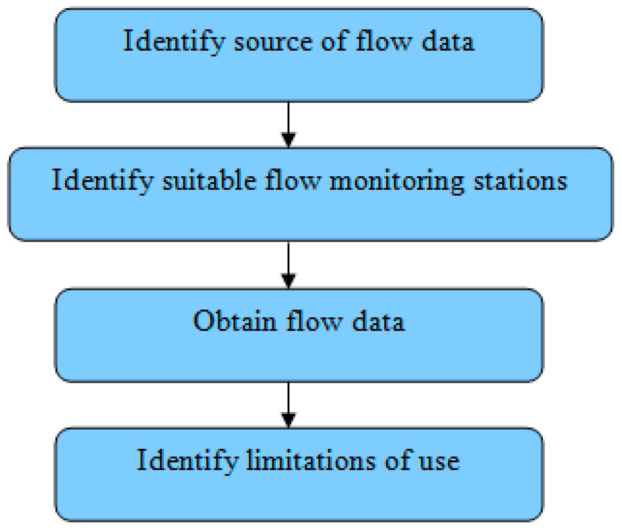
The flow data can be obtained directly from observations recorded at streamflow gauges (Figure 1), or they can be estimated using a hydrologic simulation model. The United States Geological Survey-National Water Information System (USGS-NWIS) is a major source of publicly available streamflow monitoring data for the US (http://waterdata.usgs.gov/nwis), with site selection criteria such as site name, site number, drainage area, the name of river or creek, etc.
In situations where observed flow data does not exist, flow data can be estimated from a variety of available hydrologic simulation models. While selecting the most appropriate model to obtain flow data, the user has the freedom to choose any model that is suitable for the needs of the study.
2.1.3. Step 3—Identification of Hydrologic Alteration and Division of Flow Data
The hydrologic alteration can be identified by plotting cumulative runoff against cumulative rainfall over time for the stream segment of interest. Any significant watershed disturbances (whether anthropogenic or natural alterations), such as land cover change, can alter the relationship between rainfall and runoff. However, there may be situations when the proportions of cumulative runoff are unaffected, such as base flow and surface runoff. Under these circumstances, an analysis of specific indicators targeted at low flow and high flow offers additional information. Identifying “hydrologic alteration” involves the following steps:
- Collect streamflow data,
- Collect precipitation data corresponding to flow data,
- Compute cumulative values for streamflow and precipitation data,
- Plot cumulative flow (dependent variable) on the Y-axis against cumulative precipitation (independent variable) on the X-axis,
- Identify flow trends and draw slope lines onto a graph, and
- The intersection of the slope lines indicates a significant change in the trend of cumulative runoff with respect to precipitation and indicates the hydrologic change.
2.1.4. Step 4—Use of Appropriate Tools to Generate Indices of Hydrologic Alteration and Stream Health Assessment
Software tools (e.g., IHA [43]) are available to generate flow-based indices of hydrologic alteration. The IHA tool requires daily hydrologic data for the calculation of flow-based statistics. At least 20 years of record is recommended for meaningful results for pre-impact and post-impact time periods using the IHA method [44]. The IHA method calculates a total of 67 statistical parameters covering: (1) annual summary statistics, (2) an IHA statistics summary scorecard, (3) linear regression, for identifying trends in the data, (4) IHA percentile data, and (5) daily environmental flow component (EFC) flow characterization. They include 33 IHA parameters and 34 EFC parameters. The 33 IHA parameters are categorized into five groups (described in later sections of this paper), and the different characteristics of each IHA group imply different ecological influences on streams or lakes. The IHA calculates 34 EFC parameters in five different types: low flow, extreme low flows, high flow pulses, small floods, and large floods. These five types of flow events cover the full spectrum of flow conditions that must be maintained in order to sustain riverine integrity. By default, the category values for each type is >75% for high flows, <50% for low flows, <10% for extreme low flow, two-year return flow for small floods, and 10-year return flow for large floods [30,45].
2.1.5. Step 5—Creation of a Flow Duration Curve (FDC) and Indices of Hydrologic Alteration (IHA)
This section describes the development of the flow duration curves (FDCs) and computing IHA. The flow duration curve is described here, because the stream health estimation using the eco-deficit and eco-surplus method uses it. A flow duration curve illustrates the percentage of the time, i.e., the probability, that flow in a stream will equal or exceed a particular value. A basic flow duration curve measures high flows to low flows. The X-axis represents the percentage of time (known as duration or frequency of occurrence) that a particular flow value is equaled or exceeded. The Y-axis represents the quantity of flow at a given time step, e.g., cubic feet per second (cfs), which is associated with the duration. Flow duration intervals are expressed as a percentage of exceedance, with zero corresponding to the highest stream discharge in the record (i.e., flood conditions), and 100 corresponding to the lowest (i.e., drought conditions). Measured or modeled flow data are used to develop flow duration curves.
2.1.6. Step 6—Selection of Ecologically Relevant Hydrologic Indices
All of the 33 IHA parameters (Table 1) are used for estimating stream health in this study, because these selected parameters are not very redundant, and their application is well defined in the scoring framework (DHRAM) (discussed in the next section). However, a similar application procedure is not available in DHRAM for the EFC parameters; therefore, they were not used in this study.
DHRAM uses 33 hydrologic indicators. They are divided into five groups of equal importance namely:
- Magnitude of monthly flows,
- Magnitude and duration of annual extreme flows,
- Timing of annual extreme flows,
- Frequency and duration of high and low flows, and
- Rate and frequency of change in flow conditions.
Each group of indicators has some ecological relevance that relates to stream health [29,44]. The groups of indicators are related to habitat availability for aquatic organisms, the structuring of river channel morphology, the physical habitat conditions, compatibility with life cycles of organisms, the frequency and duration of anaerobic stress for plants, and entrapment on islands and floodplains, respectively (Table 1). Therefore, by quantitatively analyzing the difference in the values of these indicators during pre-alteration and post-alteration periods, we can judge the health of the stream. It should be noted that means and coefficients of variation (CVs) are estimated for each parameter in each group.
The IHA software generates annual indicators. Hence, the annual IHA indicators must be averaged for the entire period of the record (for example, entire pre-alteration period or post-alteration period) to ascertain differences between the pre-alteration and post-alterations.
2.1.7. Step 7—Estimation of Stream Health
Two different methods are explored for estimating stream health using a time series of mean daily flow data: (1) the concept of eco-deficit versus eco-surplus using flow duration curves to estimate the presence or absence of a stream health problem, and (2) the IHA-DHRAM framework to estimate the overall health of a stream. Both of the methods are described with case examples.
Eco-Deficit and Eco-Surplus Method Using FDCs
The concept of the eco-deficit and eco-surplus method (which was originally developed for regulating flows through dams in an ecologically sustainable way) offers a simplified graphical representation of hydrologic impacts using FDCs. This is an excellent tool for interpreting the hydrologic changes overall and for making a preliminary judgment on stream health. The user can visualize the hydrologic changes and easily interpret the impacts of those hydrologic changes on stream health. It should be noted that this metric alone is insufficient to adequately capture detailed hydrologic changes, because the hydrologic variations occur in terms of magnitude, timing, duration, frequency, and rate of change. In this approach, timing and seasonality can be addressed to some extent, because the eco-deficit and eco-surplus can be computed over any period of interest (monthly, annual, or seasonal) and reflect the overall changes in streamflow [46].
The identification of a hydrologic alteration in flow data and separation of that flow data into pre-alteration and post-alteration periods are essential requirements for using this approach. FDCs have to be then prepared for pre-alteration and post-alteration conditions. Using the probability of exceedance or frequency of streamflow as a common index (X-axis), FDCs for both pre-alteration and post-alteration conditions should be plotted together. The difference between the two FDCs should be marked clearly and identified as either eco-deficit or eco-surplus. The eco-surplus or eco-deficit obtained should be interpreted for stream health conditions using Table 2 as the reference. Table 2 is developed as a part of this study.
IHA-DHRAM Approach
In order to estimate stream health and identify the extent of stream impairment, the DHRAM [31] is used as a framework. The DHRAM scoring method is designed for use with ecologically relevant hydrologic indicators (as outlined by Black et al. in 2005) generated by IHA software. However, it can also be used with similar hydrologic indicators generated by other software programs. DHRAM connects hydrologic indicators to ecological impact through the concept of risk, with the assumption that the risk to stream health increases in direct proportion to the total alteration to the hydrologic regime (or flow magnitude and pattern). The result is a DHRAM classification between one (no impact to stream health) and five (severe impact to stream health).
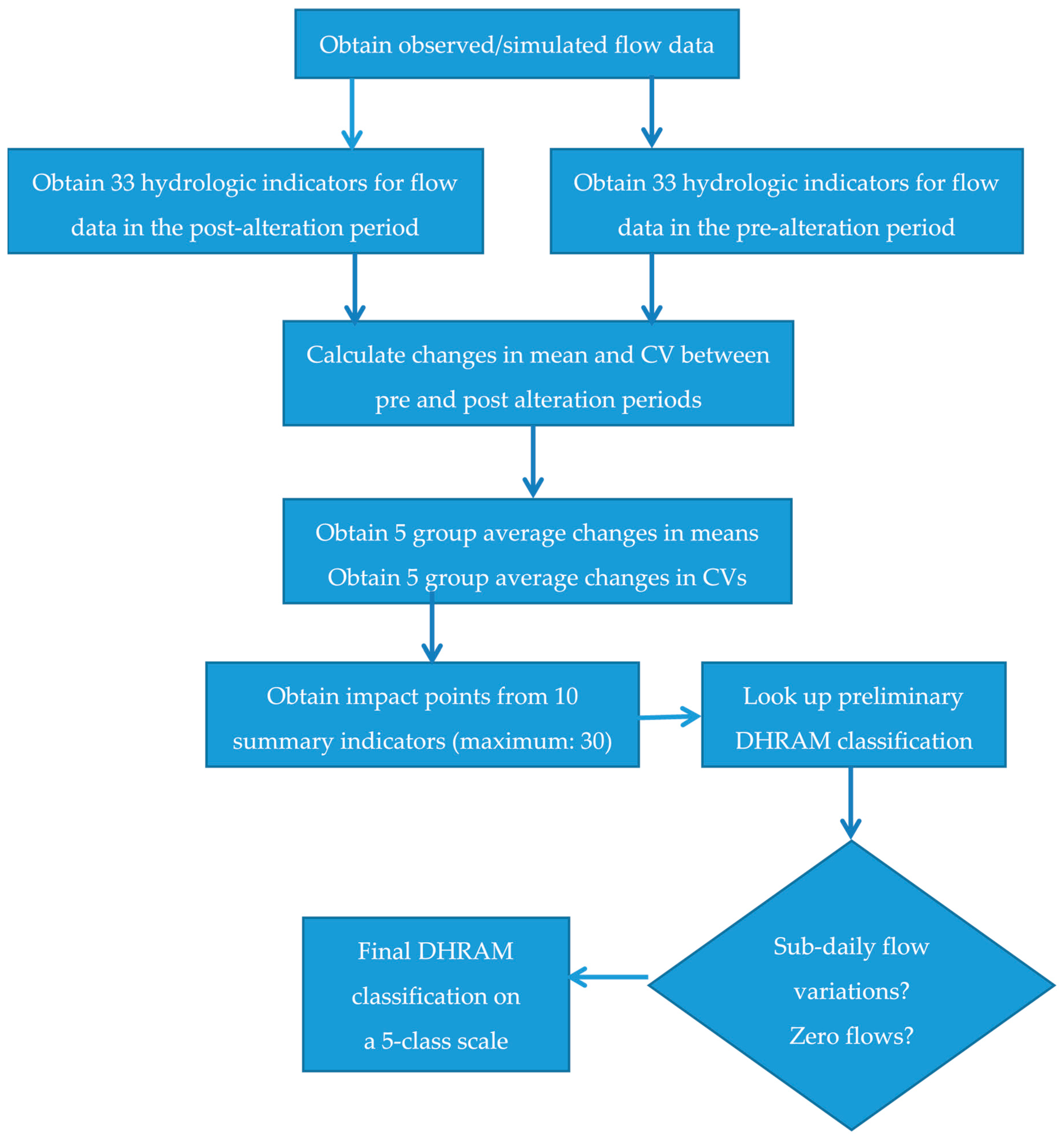
The IHA–DHRAM approach that we used to estimate stream health is presented in Figure 2. An important preliminary step in this approach is the estimation of the percentage difference between pre-alteration and post-alteration values. It is estimated as:
The percentage difference is estimated separately for means and coefficients of variation (CVs), and is summarized for each group. The percentage difference provides an estimate of the impact points, which are eventually used to estimate stream health. Then, for each group, the impact points are assigned with scores using Black et al. [31] based on known information on stream health for watersheds of varying sizes and hydrologic patterns [31]. For any stream, there will be a maximum of 10 categories (five groups and two categories in each group) to assign impact points. Each category has a maximum of three impact points. Therefore, the maximum possible total impact point is 30. Based on the total impact point for all of the groups, the streams are categorized into one of the five possible classes of stream health conditions [31]. The stream that is categorized into one of the five health classes can be downgraded by one class if the anthropogenic changes alter sub-daily flow (if analyzed) by 25% for the flow magnitude that has a 95% frequency of occurrence, or if the stream dries out as a result of the changes (Table 3). Class five is the lowest classification that can be allocated.
2.2. Study Region: White Rock Creek Watershed
The study region is the Upper White Rock Creek (UWRC) watershed located in north central Texas, covering a portion of Collin County and Dallas County. The watershed has a drainage area of 65 square miles (169 km2), and is a part of the Trinity River Basin. White Rock Lake, which is located at the outlet of the watershed, is excluded from the study area, as the study focuses on the relationship between activities in the drainage area and its impact on stream health. The predominant soils are the Houston Black soil and Austin soil (72%) that exhibit swelling and shrinking with the associated variations of water that they contain.
The watershed is located north of the downtown Dallas metropolitan area, which is being affected by the urbanization and construction of the Dallas suburbs of Richardson, Addison, Plano, and Frisco. The watershed has a semi-humid subtropical climate. The average annual rainfall is 39 inches (994 mm). Most of the rainfall occurs in winter and spring. In general, the watershed has hot, dry summers and mild winters. On average, potential annual evaporation is much higher than the rainfall, resulting in significant drawdown of surface water in the summer and dry months.
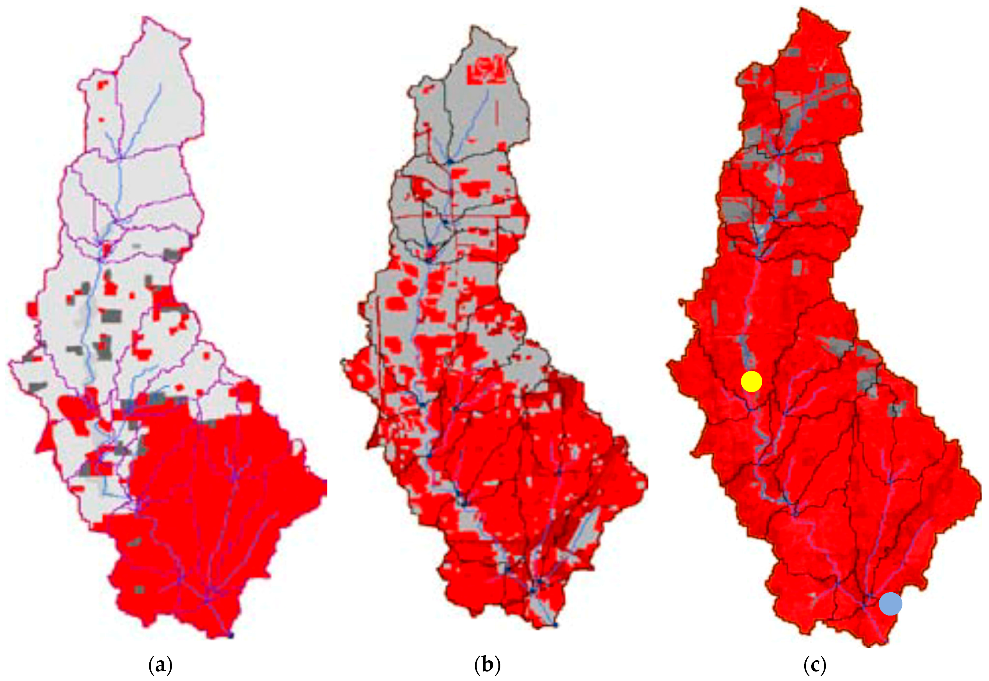
Research has found that hydrologic alteration becomes noticeable when the imperviousness hits 10% in the drainage area [22,47]. The imperviousness of the UWRC watershed increased from 41% in 1980 to 91% in 2001, according to the land cover information surveyed by the US Environmental Protection Agency (GIRAS map for 1980) and US Geological Survey (USGS) (National Land Cover Dataset (NLCD2001) [48]). Urbanization in the watershed occurred from south to north as the Dallas metropolitan expanded over time (Figure 3).
The urbanization in the middle of the watershed was more dramatic (from 2% to 92%) than the other parts during this period. Therefore, the creek was anticipated to be more altered at this point than at the watershed outlet. However, there were no monitored flow observations for this portion.
2.3. Data Used
Two US Geological Survey (USGS) gauging stations are located on Upper White Rock Creek to monitor stream flows: one at Keller Springs Road (USGS Station No. 08057100), and the other at Greenville Avenue, Dallas, Texas (USGS Station No. 08057200). The gauge at Greenville Avenue is the monitoring point at the watershed outlet. For this gauge, mean daily flow data is available from 1961 to date. However, there was a discontinuity in flow monitoring between October 1980 and March 1984. For the gauge near Keller Springs Road, flow data is available from 1961 to 1979. For estimating stream health for this watershed, daily flow data (both simulated and observed) as per the details shown in Table 4 were used with the IHA–DHRAM approach. White Rock Creek, with flow data for the period 1962–2008 at the watershed outlet, is referred to as the gauged stream. Similarly, White Rock Creek at the outlet of sub-basin 10 using simulated flow data from the SWAT model (because of incomplete observations) is referred to as the ungauged stream (Table 4).
2.4. Watershed Model Setup
A watershed model setup with a reach outlet was made using the ArcSWAT2009 interface, and flow values were generated at this point after a model calibration. A benefit of using a synthetic flow data is that the stream responses using the same weather information (25 years between 1981 and 2005 in this case) are directly compared in the analysis for both the pre-alteration and post-alteration period. Therefore, the impact of urbanization is more directly expressed in the output without the interference of climate variability. More details on the SWAT modeling of White Rock Creek is found in Kannan and Jeong [49].
3. Results and Discussion
3.1. Application of the Stream Health Estimation Approach for the Study Region
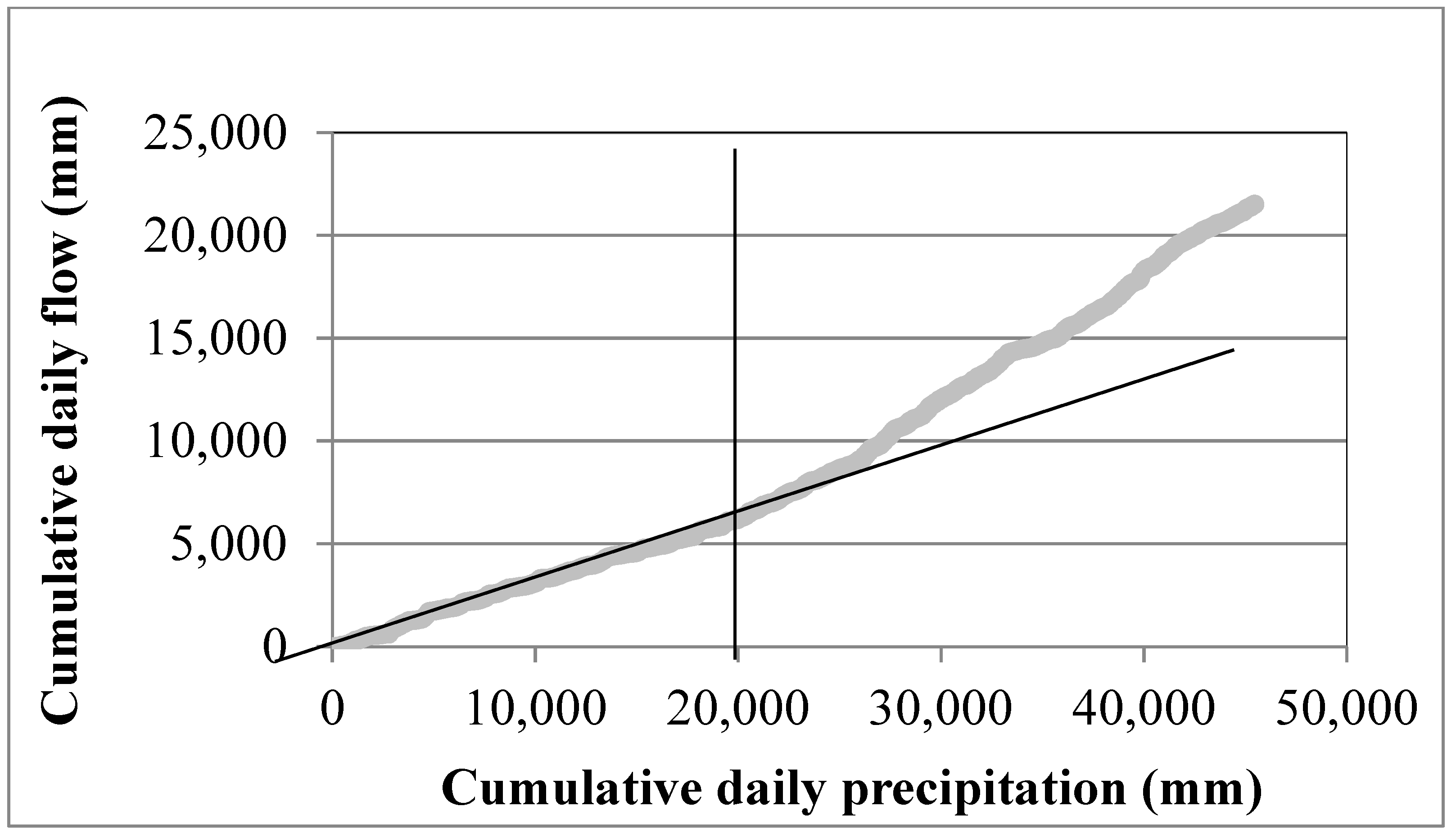
For the UWRC watershed, a significant hydrologic change was found in 1980 based on the deviation of the trends in the plot of cumulative flow to cumulative precipitation (Figure 4). Therefore, the period before 1980 was defined as the pre-alteration period, and the period after 1980 was defined as the post-alteration period.
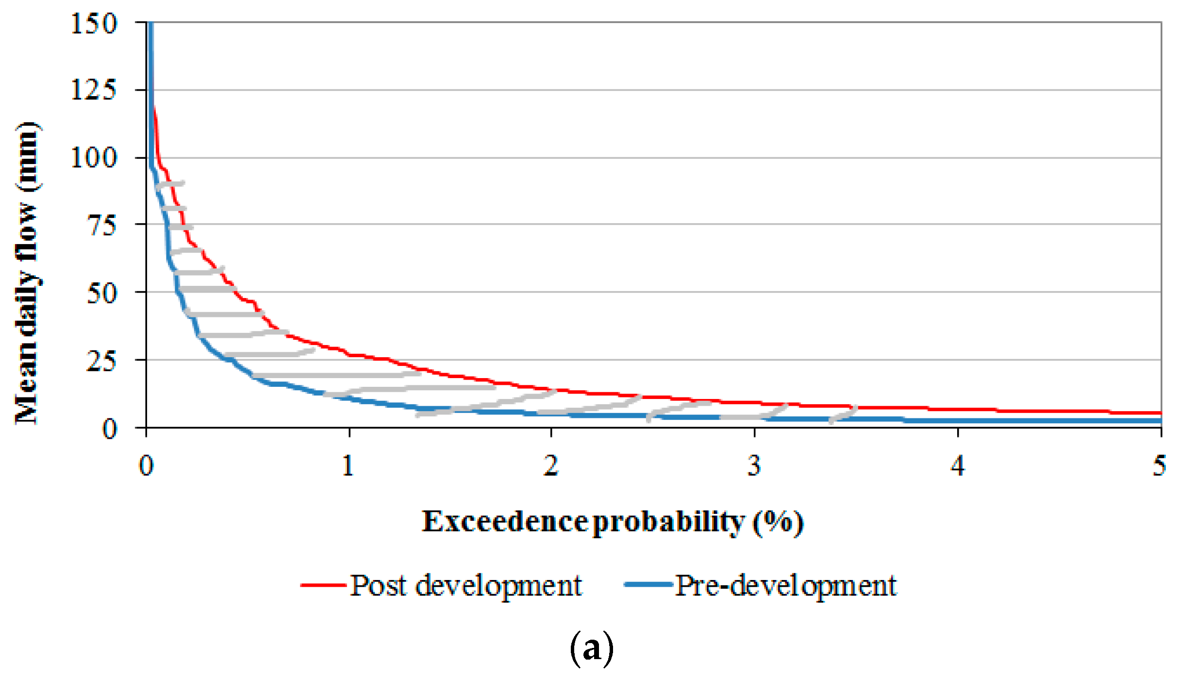
We utilized a qualitative method for identifying the existence of a stream health problem based on eco-deficit/eco-surplus methodology [19]. The general connotation when using this published methodology is that eco-surplus is good (and deficit bad), although Poff and Zimmerman [29] maintain that any change in the natural flow regime, whether higher (surplus) or lower (deficit), can impair stream health depending on the magnitude, timing, duration, frequency, and rate of change. The pre-alteration and post-alteration FDCs for White Rock Creek watershed (Figure 5) indicate that an eco-surplus exists in addition to the already discussed stream health problem (minimum to moderate in severity; Table 2), supporting Poff and Zimmerman’s [29] assertion.
3.2. Gauged Stream Using Observed Streamflow Data
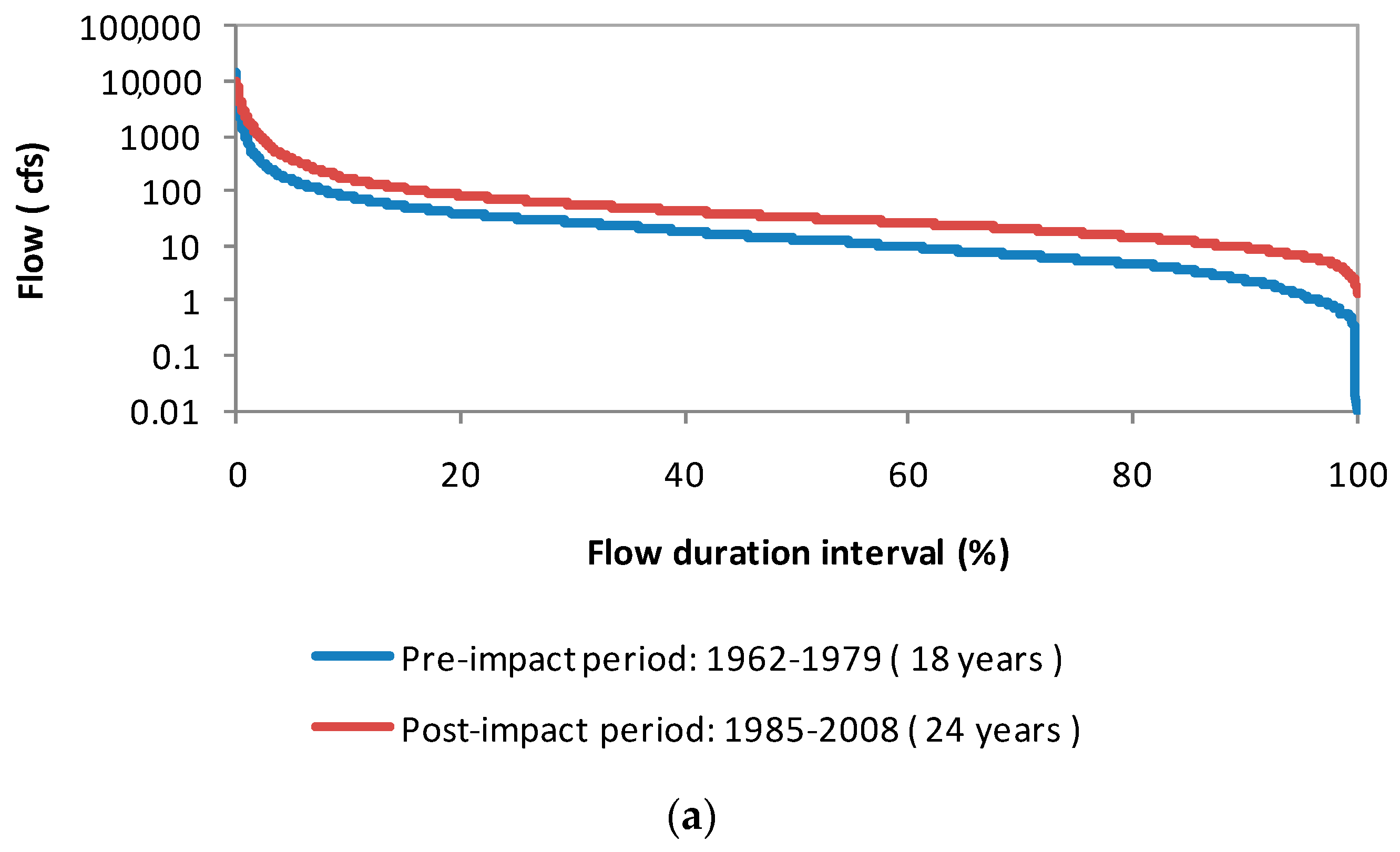
The 33 IHA parameters calculated for the pre-alteration period (1962–1979) and the post-alteration period (1984–2008) are shown in Table 5. The mean annual flow for the pre-alteration period was 55.4 cubic feet per second (cfs); for the post-alteration period, the mean annual flow was 117.1 cfs. The maximum daily flows were 14,700 cfs and 10,300 cfs for the pre-alteration and post-alteration periods, respectively. The annual CV was estimated at 5.75 (pre-alteration) and 3.82 (post-alteration). These statistics show that the increased urbanization influenced the flow volume to increase significantly, but also resulted in less variation in the flow (Figure 6a).
An examination of the IHA parameters in Table 5 provides us with the following information on the DHRAM point scores. At the watershed outlet, the mean monthly flows (IHA Group 1) and flow extreme of various durations (IHA Group 2) have increased through the year, while the frequency and duration of low pulses, and the frequency of high pulses (IHA Group 4), decreased. The increased precipitation during post-alteration (monthly average precipitation from January–December are 58.5 mm, 74.7 mm, 88.8 mm, 83.5 mm, 140.7 mm, 110.1 mm, 61.5 mm, 53.0 mm, 67.3 mm, 121.9 mm, 81.8 mm, and 77.6 mm, respectively) than pre-alteration (monthly average precipitation from January–December are 48.3 mm, 56.9 mm, 76.7 mm, 111.4 mm, 123.7 mm, 75.6 mm, 57.2 mm, 65.7 mm, 118.8 mm, 85.7 mm, 53.4 mm, and 50.1 mm, respectively) appears to be the reason for the increases in the parameters in Groups 1 and 2, but the decline in Group 4 parameters with increased rainfall does not occur naturally. It is suggested that it may be the effects of flood control structures such as small dams and ponds that retard stormwater before releasing it downstream.
The DHRAM analysis (Table 6) shows that the stream health at the watershed outlet is in Class 3, which indicates a moderate risk of impact. Maximum impact points were obtained for Group 1 indicators, which are related to the magnitude of monthly water conditions. Possible ecosystem influences regarding the Group 1 include:
- Habitat availability for aquatic organisms
- Soil moisture availability for plants
- Availability of water for terrestrial animals
- Availability of food/cover for fur-bearing mammals
- Reliability of water supplies for terrestrial animals
- Access by predators to nesting sites
- Influences water temperature, oxygen levels, photosynthesis in the water column.
3.3. Ungauged Stream Using Model Simulated Streamflow Data
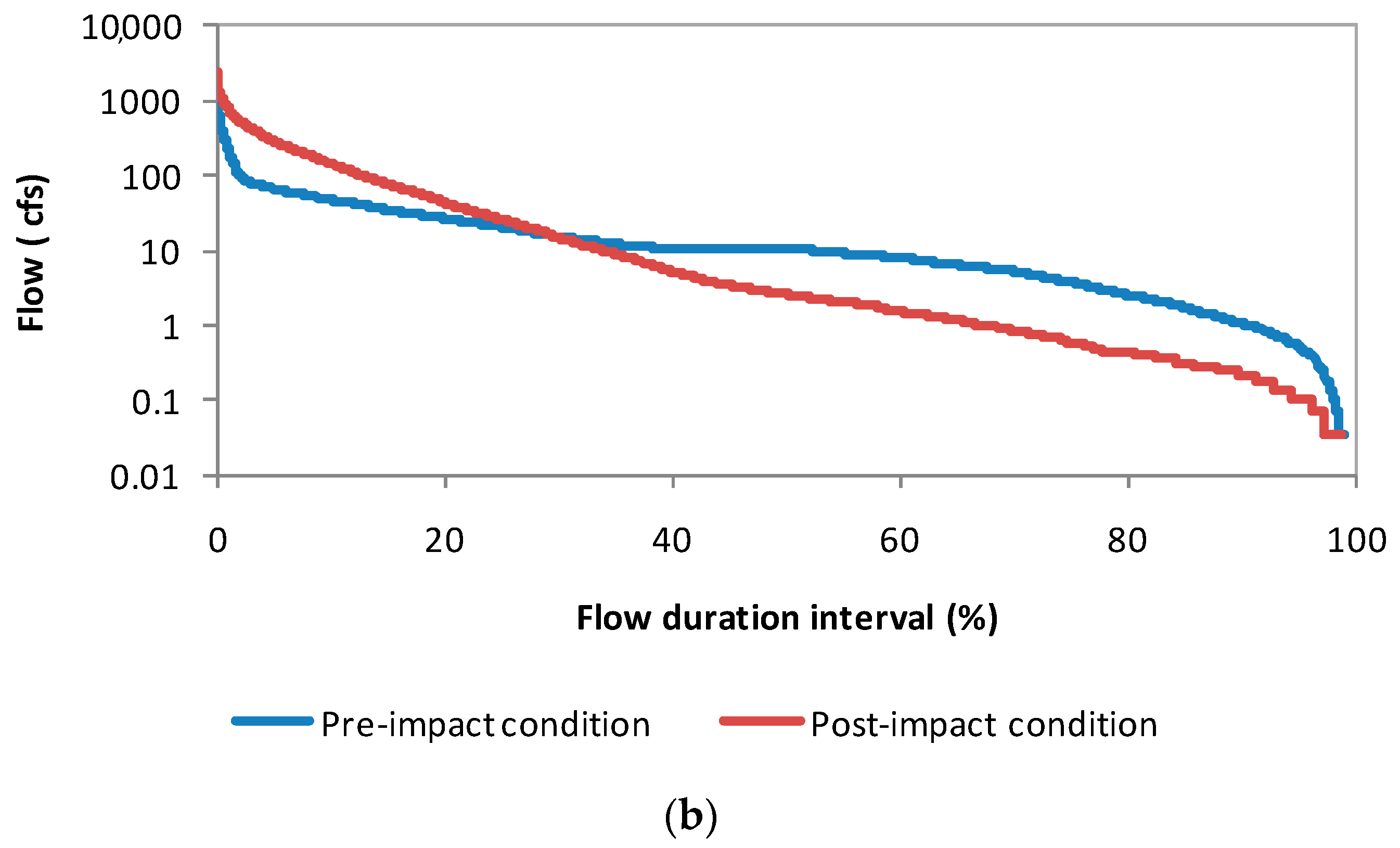
No flow records are available for the middle portion of the watershed where the urbanization was the highest. Synthetic flow data were therefore used for both the pre-alteration and post-alteration periods using the SWAT model and historical land-use maps. The mean annual flow for the pre-alteration period was 21.9 cfs, and that for the post-alteration period was 53.3 cfs. The maximum daily flow was 1527 cfs and 2493 cfs, respectively. The annual CV was estimated at 2.8 (pre-alteration) and 2.96 (post-alteration). The lower variations may result from underestimated high floods by SWAT. The extreme urbanization that occurred during the two decades resulted in an increase of high flows and a decrease in the medium to low flows (Figure 6b).
The synthetic flow data predicted 18 days without flow in the creek with the pre-alteration condition, but it reduced to 11 days during the post-alteration period. The runoff from increased urban areas may contribute to this result, with a small amount of discharge into the creek. Though skipped in this study due to the lack of sub-daily flow data, the interim classification should be affected by sub-daily flow variations, if available. The final stream classification for sub-basin 10 was Class 4, which indicated a high risk of impact (Table 6).
The DHRAM analysis for sub-basin 10 scored the highest in IHA Group 4, which related to the frequency and duration of high and low pulses. Possible influences on the stream health include:
- Frequency and magnitude of soil moisture stress for plants
- Frequency and duration of anaerobic stress for plants
- Availability of floodplain habitats for aquatic organisms
- Nutrient and organic matter exchanges between river and floodplain
- Soil mineral availability
- Access for water birds to feeding, resting, and reproduction sites
- Influences bedload transport, channel sediment textures, and duration of substrate disturbance (high pulses)
The result of sub-basin 10 is straightforward and consistent with typical urbanization impacts. The intervention of climatic variability was minimal. The increased imperviousness causes an overall increase of high flow and floods with the enhanced stormwater runoff from urban pavements. Due to the disconnection in a large area between the surface and subsurface by impervious pavement, less water infiltrates into the aquifer, causing reduced groundwater recharge. Ultimately, this leads to a decrease in base flow, since the base flow component is significant in low flow regimes. This theory is supported by the changes in IHA parameters. The mean monthly flows decreased, while the flow maxima of various durations increased. Also, the frequency and duration of high/low pulses increased.
The relatively dramatic urbanization rate during the study period at sub-basin 10 (from 2% to 91%), compared to the watershed outlet (from 41% to 91%), is somewhat represented in the DHRAM output. Also, this result implies that the hydrological impact of urbanization on the stream occurred in earlier stages of the development, which is consistent with previous findings [47].
3.4. Validation of Estimated Stream Health (with Our Approach) with Respect to Other Observed Physicochemical Indicators Describing the Quality of the Stream
Water quality observations recorded at Greenville Avenue, Dallas, Texas (USGS Station No. 08057200) were analyzed during pre-development and post-development periods (Table 7) in order to validate the deterioration of stream health, as suggested by the hydrologic indices-based approach used in this study. The water quality observations considered for our analysis include total dissolved solids (TDS), as well as the nitrate, chloride, and sulfate recorded during the pre-development and post-development periods (Table 7). It should be noted that the observations on pre-development were limited to one year (1969) only. Water quality observations during the post-development period showed overall stream deterioration (except nitrate). The TDS during post-development were much high than those in the pre-development period. This trend is typical to urbanization, which facilitates the easier transport of dissolved solids to the stream. Similar trends were documented by Mikalsen [50]. Chloride concentration during post-development (urbanization) is higher than pre-development, suggesting stream deterioration. The excess chlorides could have come from the chlorine that is used in water and wastewater treatment in urban areas, the drainage of swimming pools, and the diffuse source transfer of deicing salts that are used in urban areas during winter, as documented in Peter [51]. The higher values of sulfate during the post-development period compared with the pre-development period are not significant, but they are noticeable. The nitrate during post-development was lower than the nitrate present in the pre-development period. During pre-development, the stream had high levels of nitrates coming from land-applied fertilizers (from the cultivated area) and manure fate and transport (from range or forest areas). The cultivated area and forest/range are now urbanized drastically, reducing the opportunities for nitrate transport to the stream. However, there is another possible source for the nitrates with urbanization, which is the point source discharge that is typical of urban areas. However, the majority of it could have been taken care of in a water treatment plant downstream. In summary, in conjunction with all of the water quality parameters, the alterations in flow patterns, magnitude, frequency, and timings, the stream at White Rock Creek underwent stream health deterioration. This could have been additionally verified by the observation of aquatic species within the stream, and alterations in riparian vegetation along the stream during a long period spanning pre-alteration to post-alteration periods. This was not carried out because of a lack of data availability.
3.5. Stream Health Indicators for Vulnerability Assessments and Adaptation Studies in a Changing Climate
Stream health can be a powerful indicator for assessing the susceptibility of streams and their inability to cope with adverse effects of stress. Examples of stressors that streams are exposed to can be the changing land use, such as increased urbanization, as well as a changing climate. When used as an indicator in these assessments, stream health characterizes the stream’s internal characteristics, such as how the streams adjust to stressors—which represents its adaptive capacity—as well as the response of the stream to these stressors, which represents its sensitivity. These characteristics are important aspects of vulnerability assessments [7]. Vulnerability assessments using stream health indicators can be considered prerequisite information for adaptation. Adaptation is a key feature of sustainable water resource systems. Stream health can also be a powerful indicator for the adaptation of streams to various stressors by providing useful information on how the streams are responding to the unavoidable impacts of stressors while utilizing the benefits of changes that come about due to them. The adaptation of the water resources has become a core element of climate policy and research, and is important in developing adaptation strategies to mitigate the changes caused by stressors such as climate change and land-use change.
4. Summary and Conclusions
By developing a procedure to estimate stream health using daily streamflow, this study addresses the need for literature on clear guidelines for estimating stream health. Stream health can be a powerful indicator for vulnerability assessments and the development of adaptation strategies for streams. In this study, an approach was developed to estimate the stream health in aggregate, including all of the components of stream health such as riparian vegetation, aquatic species, and benthic organisms. The approach was demonstrated with a case study.
- Upper White Rock Creek watershed (UWRC) in Texas, US was chosen as the study area because it presented a classic case of progressive urbanization.
- Monitored flow observations at the watershed outlet and simulated flow results from a watershed-scale computer model were used for the generation of hydrologic indices explaining various stream health parameters.
- The flow dataset was divided into pre-urbanization and post-urbanization parts after identifying major changes in hydrologic trends from 1980 onwards.
- Indices of Hydrologic Alteration (IHA) software was used to generate statistics on flow data (flow-based indices) separately for pre-alteration and post-alteration periods. The Dundee Hydrologic Regime Assessment Method (DHRAM) was used as the framework and scoring system for the estimation of stream health.
- Flow duration curves were developed for pre-alteration and post-alteration periods for the qualitative estimation of the presence or absence of stream health problems in the watershed.
- All 33 IHA parameters were used for analyzing stream health, because the scoring system was well-defined in the DHRAM for these IHA parameters.
- Stream health impacts were analyzed for White Rock Creek watershed using the 33 IHA parameters and the scoring system in the DHRAM for the watershed outlet and sub-basin outlet 10 (which presented the classical urbanization problem). The watershed outlet and outlet of sub-basin 10 received impact scores of 3 and 4, respectively.
- The stream health was estimated to be moderately impacted at the watershed outlet and moderate to severely impacted at the outlet of sub-basin 10.
The hydrologic consequences of land cover change, urbanization, and other human-made activities were reflected in the values of hydrologic indices estimated for pre-alteration and post-alteration periods. The deterioration of stream health in the White Rock Creek Watershed (as estimated by our approach) is confirmed by an analysis of the physicochemical water quality parameters observed for the stream over a period of years. The procedure outlined in the study estimated stream health results that were consistent with other sources. Also, the nature of results was expected, given the nature and extent of changes that occurred in the watershed. For further research, it is recommended to test the approach for other rivers in the US, and possibly watersheds in other countries. The procedure could also be integrated with a modeling tool for the estimation of stream health for ungauged streams. Full automation of the procedure could be another option to continue this research. Based on the results obtained, the following conclusions can be drawn:
- With the use of the eco-deficit and eco-surplus method, we were able to identify the existence of a stream health problem in the UWRC due to urbanization. The existence of the stream health problem in the UWRC was validated with the help of water quality samples monitored during pre-alteration and post-alteration periods. Therefore, based on the results of our study, we can conclude that the eco-deficit and eco-surplus method could be a used as a screening tool to identify the existence of stream health problems in a stream. However, other methods also need to be used to find out more details about the stream health problems.
- Using the IHA–DHRAM framework, we were able to correctly categorize sub-basin 10 (where the dramatic urbanization occurred in the watershed) with a high risk of stream health impact, and the watershed outlet with a moderate risk of stream health impact. Given the extent of urbanization (Figure 3) in different sections of the watershed, the stream health categorization makes sense. Therefore, it appears from our results that the IHA–DHRAM approach could be used to estimate the health of streams in other places, too.
- Simulated streamflow results from modeling tools could be successfully used to estimate the presence/absence of stream health problems using the eco-deficit and eco-surplus approach, and more details on the stream health problem using the IHA–DHRAM framework. The tools identified and the stepwise procedure outlined in our study could be easily adopted for other streams in the United States and elsewhere.
Acknowledgments
This project was carried out by Texas AgriLife Research at Blackland Research and Extension Center, Temple, TX, US with funding from the United States-Environmental Protection Agency (USEPA) Region VI. The authors wish to thank the USEPA for funding this work.
Author Contributions
For Narayanan Kannan conceived and designed the entire study and validated the stream health estimation with water quality observations; Jaehak Jeong performed the stream health estimation; Aavudai Anandhi brought in the concept of vulnerability assessment and adaptation related to stream health and wrote a considerable portion of the manuscript; All the authors contributed to the writing of the manuscript.
Conflicts of Interest
The authors declare no conflict of interest. The funding sponsors had no role in the design of the study; in the data collection, analyses.
References
- Woznicki, S.A.; Nejadhashemi, A.P.; Ross, D.M.; Zhang, Z.; Wang, L.; Esfahanian, A.-H. Ecohydrological model parameter selection for stream health evaluation. Sci. Total Environ. 2015, 511, 341–353. [Google Scholar] [CrossRef] [PubMed]
- Harmsworth, G.; Young, R.; Walker, D.; Clapcott, J.; James, T. Linkages between cultural and scientific indicators of river and stream health. N. Z. J. Mar. Freshw. Res. 2011, 45, 423–436. [Google Scholar] [CrossRef]
- Meyer, J.L. Stream health: Incorporating the human dimension to advance stream ecology. J. N. Am. Benthol. Soc. 1997, 16, 439–447. [Google Scholar] [CrossRef]
- Vugteveen, P.; Leuven, R.; Huijbregts, M.; Lenders, H. Redefinition and elaboration of river ecosystem health: Perspective for river management. In Living Rivers: Trends and Challenges in Science and Management; Springer: Dordrecht, The Netherlands, 2006; pp. 289–308. [Google Scholar]
- Karr, J.R. Defining and measuring river health. Freshw. Biol. 1999, 41, 221–234. [Google Scholar] [CrossRef]
- Zhao, Y.; Yang, Z. Integrative fuzzy hierarchical model for river health assessment: A case study of Yong River in Ningbo City, China. Commun. Nonlinear Sci. Numer. Simul. 2009, 14, 1729–1736. [Google Scholar] [CrossRef]
- Anandhi, A. Growing degree days—Ecosystem indicator for changing diurnal temperatures and their impact on corn growth stages in Kansas. Ecol. Indic. 2016, 61, 149–158. [Google Scholar] [CrossRef]
- Anandhi, A.; Steiner, J.L.; Bailey, N. A system’s approach to assess the exposure of agricultural production to climate change and variability. Clim. Chang. 2016, 136, 647–659. [Google Scholar] [CrossRef]
- Anandhi, A.; Hutchinson, S.; Harrington, J., Jr.; Rahmani, V.; Kirkham, M.B.; Rice, W.C. Changes in spatial and temporal trends in wet, dry, warm and cold spell length or duration indices in Kansas, USA. Int. J. Climatol. 2016, 36, 4085–4101. [Google Scholar] [CrossRef]
- Bradbury, J.P.; Van Metre, P.C. A land-use and water-quality history of White Rock Lake reservoir, Dallas, Texas, based on paleolimnological analyses. J. Paleolimnol. 1997, 17, 227–237. [Google Scholar] [CrossRef]
- Dos Santos, D.; Molineri, C.; Reynaga, M.; Basualdo, C. Which index is the best to assess stream health? Ecol. Indic. 2011, 11, 582–589. [Google Scholar] [CrossRef]
- Jeong, J.; Kannan, N.; Arnold, J.G. Effects of urbanization and climate change on stream health in north-central Texas. J. Environ. Qual. 2014, 43, 100–109. [Google Scholar] [CrossRef] [PubMed]
- Lynch, A.J.; Myers, B.J.E.; Chu, C.; Eby, L.A.; Falke, A.F.; Kovach, R.P.; Krabbenhoft, T.J.; Kwak, T.J.; Lyons, J.; Paukert, C.P.; et al. Climate Change Effects on North American Inland Fish Populations and Assemblages. Fisheries 2016, 41, 346–361. [Google Scholar] [CrossRef]
- Mathon, B.R.; Rizzo, D.M.; Alexander, K.G.; Fiske, S.; Langdon, R.; Stevens, L. Assessing Linkages in Stream Habitat, Geomorphic Condition, and Biological Integrity Using a Generalized Regression Neural Network. J. Am. Water Resour. Assoc. 2013, 49, 415–430. [Google Scholar] [CrossRef]
- Nejadhashemi, A.P.; Zhang, Z.; Herman, M.R.; Shortridge, A.; Marquart-Pyatt, S. Evaluating stream health based environmental justice model performance at different spatial scales. J. Hydrol. 2016, 538, 500–514. [Google Scholar] [CrossRef]
- Gazendam, E.; Gharabaghi, B.; Ackerman, J.D.; Whiteley, H. Integrative neural networks models for stream assessment in restoration projects. J. Hydrol. 2016, 536, 339–350. [Google Scholar] [CrossRef]
- Agouridis, C.T.; Weslye, E.T.; Sanderson, T.M. Aquatic Macroinvertebrates: Biological Indicators of Stream Health; Cooperative Extension Service; University of Kentucky College of Agriculture: Lexington, KY, USA, 2014. [Google Scholar]
- Cruse, R.; Huggins, D.; Lenhart, C.; Magner, J.; Royer, T.; Schilling, K. Assessing the Health of Streams in Agricultural Landscapes: The Impacts of Land Management Change on Water Quality; Special Publication, No. 31; Council for Agricultural Science and Technology: Ames, IA, USA, 2012. [Google Scholar]
- Gao, Y.; Vogel, R.M.; Kroll, C.N.; Poff, N.L.; Olden, J.D. Development of representative indicators of hydrologic alteration. J. Hydrol. 2009, 374, 136–147. [Google Scholar] [CrossRef]
- United States Department of Agriculture, Natural Resources Conservation Service (USDA-NRCS). Stream Visual Assessment Protocol; Technical Note 99-1; National Water and Climate Center (NWCC): Portland, OR, USA, 1998. [Google Scholar]
- DeGasperi, C.L.; Berge, H.B.; Whiting, K.R.; Burkey, J.J.; Cassin, J.L.; Fuerstenberg, R.R. Linking hydrologic alteration to biological impairment in urbanizing streams of the Puget Lowland, Washington, USA. J. Am. Water Resour. Assoc. 2009, 45, 512–533. [Google Scholar] [CrossRef] [PubMed]
- Wang, L.Z.; Lyons, J.; Kanehl, P. Impacts of urbanization on stream habitat and fish across multiple spatial scales. Environ. Manag. 2001, 28, 255–266. [Google Scholar] [CrossRef]
- Morse, C.C.; Huryn, A.D.; Cronan, C. Impervious Surface Area as a Predictor of the Effects of Urbanization on Stream Insect Communities in Maine, U.S.A. Environ. Monit. Assess. 2003, 89, 95–127. [Google Scholar] [CrossRef] [PubMed]
- Booth, D.B.; Karr, J.R.; Schauman, S.; Konrad, C.P.; Morley, S.A.; Larson, M.G.; Burges, S.J. Reviving Urban Streams: Land Use, Hydrology, Biology, and Human Behavior. J. Am. Water Resour. Assoc. 2004, 40, 1351–1364. [Google Scholar] [CrossRef]
- Walsh, C.J. Protection of In-Stream Biota from Urban Impacts: Minimize Catchment Imperviousness or Improve Drainage Design? Mar. Freshw. Res. 2004, 55, 317–326. [Google Scholar] [CrossRef]
- Konrad, C.P.; Booth, D.B. Hydrologic Changes in Urban Streams and Their Ecological Significance. Am. Fish. Soc. Symp. 2005, 47, 157–177. [Google Scholar]
- Walsh, C.J.; Roy, A.H.; Feminella, J.W.; Cottingham, P.D.; Groffman, P.M.; Morgan, R.P., II. The Urban Stream Syndrome: Current Knowledge and the Search for a Cure. J. N. Am. Benthol. Soc. 2005, 24, 706–723. [Google Scholar] [CrossRef]
- Pradhanang, S.M.; Mukundan, R.; Schneiderman, E.M.; Zion, M.S.; Anandhi, A.; Pierson, D.C.; Frei, A.; Easton, Z.M.; Fuka, D.; Steenhuis, T.S. Streamflow responses to climate change: Analysis of hydrologic indicators in a New York City water supply watershed. J. Am. Water Resour. Assoc. 2013, 49, 1308–1326. [Google Scholar] [CrossRef]
- Poff, N.L.; Zimmerman, J.K.H. Ecological responses to altered flow regimes: A literature review to inform the science and management of environmental flows. Freshw. Biol. 2010, 55, 194–207. [Google Scholar] [CrossRef]
- The Nature Conservancy. Indicators of Hydrologic Alteration—Version 7 User’s Manual; The Nature Conservancy: Arlington, VA, USA, 2007. [Google Scholar]
- Black, A.R.; Rowan, J.S.; Duck, R.W.; Bragg, O.M. DHRAM: A method for classifying river flow regime alterations for the EC Water Framework Directive. Aquat. Conserv. Mar. Freshw. Ecosyst. 2005, 15, 427–446. [Google Scholar] [CrossRef]
- Baker, D.B.; Richards, R.P.; Loftus, T.T.; Kramer, J.W. A New Flashiness Index: Characteristics and Applications to Midwestern Rivers and States. J. Am. Water Resour. Assoc. 2004, 40, 504–522. [Google Scholar] [CrossRef]
- Benjamin, L.; Van Kirk, R.W. Assessing instream flows and reservoir operations on an eastern Idaho river. J. Am. Water Resour. Assoc. 1999, 35, 898–909. [Google Scholar] [CrossRef]
- Brunke, M. Floodplains of a regulated southern alpine river (Brenno, Switzerland): Ecological assessment and conservation options. Aquat. Conserv. Mar. Freshw. Ecosyst. 2002, 12, 583–599. [Google Scholar] [CrossRef]
- Galat, D.L.; Lipkin, R. Restoring ecological integrity of great rivers: Historical hydrographs aid in defining reference conditions for the Missouri River. In Assessing the Ecological Integrity of Running Waters; Series Developments in Hydrobiology; Springer: Dordrecht, The Netherlands, 2000; Volume 149, pp. 29–48. ISBN 978-94-011-4164-2. [Google Scholar]
- Gergel, S.E.; Turner, M.G.; Miller, J.R.; Melack, J.M.; Stanley, E.H. Landscape indicators of human impacts to riverine systems. Aquat. Sci. 2002, 64, 118–128. [Google Scholar] [CrossRef]
- Koel, T.M.; Sparks, R.E. Historical patterns of river stage and fish communities as criteria for operations of dams on the Illinois River. River Res. Appl. 2002, 18, 3–19. [Google Scholar] [CrossRef]
- Armstrong, D.S.; Parker, G.W.; Richards, G.W. Evaluation of Streamflow Requirements for Habitat Protection by Comparison to Streamflow Characteristics at Index Streamflow-Gaging Stations in Southern New England; Water-Resources Investigations Report 03-4332; U.S. Department of Interior; U.S. Geological Survey: Reston, VA, USA, 2004.
- Irwin, E.R.; Freeman, M.C. Proposal for Adaptive Management to Conserve Biotic Integrity in a Regulated Segment of the Tallapoosa River, Alabama, USA. Conserv. Biol. 2002, 16, 1212–1222. [Google Scholar] [CrossRef]
- Shiau, J.T.; Wu, F.C. Assessment of hydrologic alterations caused by Chi-Chi diversion weir in Chou-Shui Creek, Taiwan. River Res. Appl. 2004, 20, 401–412. [Google Scholar] [CrossRef]
- Stewardson, M.J.; Gippel, C.J. Incorporating Flow Variability into Environmental Flow Regimes Using the Flow Events Method. River Res. Appl. 2003, 19, 459–472. [Google Scholar] [CrossRef]
- Tharme, R.E. A Global Perspective on Environmental Flow Assessment: Emerging Trends in the Development and Application of Environmental Flow Methodologies for Rivers. River Res. Appl. 2003, 19, 397–441. [Google Scholar] [CrossRef]
- IHA Software Download. Available online: https://www.conservationgateway.org/ConservationPractices/Freshwater/EnvironmentalFlows/MethodsandTools/IndicatorsofHydrologicAlteration/Pages/IHA-Software-Download.aspx (accessed on 14 March 2018).
- Richter, B.D.; Baumgartner, J.V.; Powell, J.; Braun, D.P. A method for assessing hydrologic alteration within ecosystems. Conserv. Biol. 1996, 10, 1163–1174. [Google Scholar] [CrossRef]
- Swanson, S. Resource Notes: Indicators of Hydrologic Alteration. Hydrology; National Science and Technology Center, Bureau of Land Management: Denver, CO, USA, 2002; p. 58.
- Vogel, R.M.; Sieber, J.; Archfield, S.A.; Smith, M.P.; Apse, C.D.; Huber-Lee, A. Relations among storage, yield, and instream flow. Water Resour. Res. 2007, 43, 1–12. [Google Scholar] [CrossRef]
- Booth, D.B.; Jackson, C.R. Urbanization of aquatic systems: Degradation thresholds, storm water detection, and the limits of mitigation. J. Am. Water Resour. Assoc. 1997, 33, 1077–1090. [Google Scholar] [CrossRef]
- Homer, C.; Dewitz, J.; Fry, J.; Coan, M.; Hossain, N.; Larson, C.; Herold, N.; McKerrow, A.; VanDriel, J.N.; Wickham, J. Completion of the 2001 National Land Cover Database for the Conterminous United States. Photogramm. Eng. Remote Sens. 2007, 73, 337–341. [Google Scholar]
- Kannan, N.; Jeong, J. An Approach for Estimating Stream Health Using Flow Duration Curves and Indices of Hydrologic Alteration; Report Prepared for the United States Environmental Protection Agency-Retion 6; United States Environmental Protection Agency Office of Water: Dallas, TX, USA, 2011.
- Mikalsen, T. Causes of Increased Total Dissolved Solids and Conductivity Levels in Urban Streams in Georgia. In Proceedings of the 2005 Georgia Water Resources Conference, Athens, GA, USA, 25–27 April 2005; Hatcher, K.J., Ed.; Institute of Ecology, University of Georgia: Athens, GA, USA, 2005. [Google Scholar]
- Peter, N.E. Effects of urbanization on stream water quality in the city of Atlanta, Georgia, USA. Hydrol. Process. 2009, 23, 2860–2878. [Google Scholar] [CrossRef]
Figure 1.
Approach for obtaining data from monitored observations.

Figure 2.
Estimating Stream Health using IHA–DHRAM Approach (IHA is Indices of Hydrologic Alteration, and DHRAM is Dundee Hydrologic Regime Assessment Method).
Figure 2.
Estimating Stream Health using IHA–DHRAM Approach (IHA is Indices of Hydrologic Alteration, and DHRAM is Dundee Hydrologic Regime Assessment Method).

Figure 3.
History of urbanization in the White Rock Creek watershed (areas colored in red indicate urbanization in the watershed; the yellow circle is the gauge located at Keller Springs Road (United States Geological Survey, or USGS, Station No. 08057100), which corresponds to the outlet of sub-basin 10 (ungauged); the aqua blue circle is the gauge located at Greenville Avenue (USGS Station No. 08057200), which corresponds to the watershed outlet (gauged). (a) 1980: 41% urban; (b) 1990: 57% urban; (c) 2001: 91% urban.

Figure 4.
Hydrologic alteration for White Rock Creek watershed (the thick grey line represents a trend of cumulative runoff with respect to cumulative precipitation; the intersection of thin black lines (in relation to the thick grey line) indicates significant change in the trend of cumulative runoff with respect to precipitation). Period of data for precipitation and streamflow: 1962–2007. Flow data used for this analysis is located at Greenville Avenue, Dallas, Texas (USGS Station No. 08057200).

Figure 5.
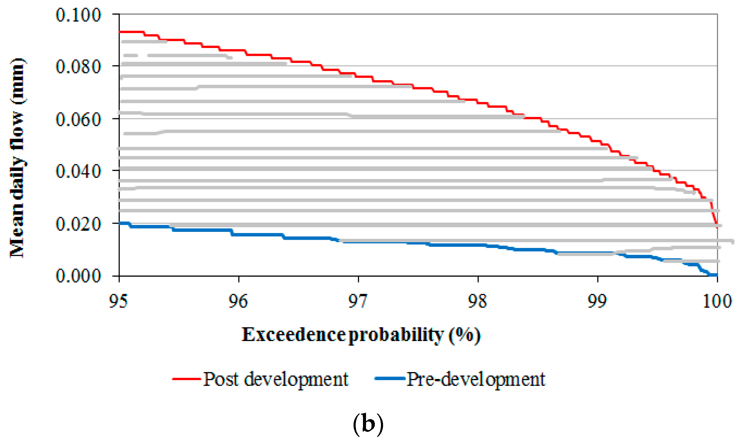
(a) Eco-surplus in a high-flow portion of the FDC for the White Rock Creek watershed (eco-surplus is the net volume of water now available that is above the pre-development conditions). (b) Eco-surplus in low-flow portion of the FDC for the White Rock Creek watershed (eco-surplus is the net volume of water now available that is above the pre-development conditions).
Figure 5.
(a) Eco-surplus in a high-flow portion of the FDC for the White Rock Creek watershed (eco-surplus is the net volume of water now available that is above the pre-development conditions). (b) Eco-surplus in low-flow portion of the FDC for the White Rock Creek watershed (eco-surplus is the net volume of water now available that is above the pre-development conditions).


Figure 6.
(a) Impact of urbanization on streamflow in the White Rock Creek watershed at the watershed outlet; (b) Impact of urbanization on streamflow in the White Rock Creek watershed at sub-basin 10.
Figure 6.
(a) Impact of urbanization on streamflow in the White Rock Creek watershed at the watershed outlet; (b) Impact of urbanization on streamflow in the White Rock Creek watershed at sub-basin 10.


Table 1.
List of Indicators of Hydrologic Alteration (IHA) Parameters Chosen for the Estimation of Stream Health and their Importance.
Table 1.
List of Indicators of Hydrologic Alteration (IHA) Parameters Chosen for the Estimation of Stream Health and their Importance.
| Group | Parameter Details | Total Number of Parameters | Importance |
|---|---|---|---|
| 1 | Magnitude of monthly flow Average flow for each month Jan–Dec | 12 | Habitat availability for aquatic organisms, availability of water for terrestrial animals |
| 2 | Magnitude and duration of annual extremes Minimum and maximum of 1, 3, 7, 30, and 90-day flow | 12 | Structuring of aquatic ecosystems by abiotic vs. biotic factors, structuring of river channel morphology and physical habitat conditions, soil moisture stress in plants |
| 3 | Timing of annual extreme flow Dates of daily maximum and minimum flow | 2 | Compatibility with life cycles of organisms |
| 4 | Frequency and duration of high and low flow pulses Number of low and high pulses in each year Mean/median of low and high pulse durations | 4 | Frequency/duration of anaerobic stress for plants, availability of floodplain habitats |
| 5 | Rate and frequency of change in flow Rates of rise and fall and number of hydrologic reversals | 3 | Drought stress on plants, entrapment on islands and floodplains |
Table 2.
Estimating Stream Health by Interpreting Eco-Deficit and Eco-Surplus Information of Flow Duration Curves (FDCs) (D-Deficit and S-Surplus).
Table 2.
Estimating Stream Health by Interpreting Eco-Deficit and Eco-Surplus Information of Flow Duration Curves (FDCs) (D-Deficit and S-Surplus).
| Possible Scenarios | High Flow Portion (Head) of FDC | Low Flow Portion (Tail) of FDC | Stream Health Problems | ||
|---|---|---|---|---|---|
| Eco-Surplus | Eco-Deficit | Eco-Surplus | Eco-Deficit | ||
| SS | Small | Small | None or Minimal | ||
| SS | Big | Big | Minimal to Moderate | ||
| SD | Small | Small | Minimal | ||
| SD | Big | Big | Moderate to High | ||
| DD | Small | Small | Minimal | ||
| DD | Big | Big | Moderate to High | ||
| DS | Small | Small | None or Minimal | ||
| DS | Big | Big | Moderate to High | ||
Table 3.
DHRAM Classes and Stream Health Impact Categories.
| Class | Range of Points | Impact Category |
|---|---|---|
| 1 | 0 | Unimpacted condition |
| 2 | 1–4 | Low risk of impact |
| 3 | 5–10 | Moderate risk of impact |
| 4 | 11–20 | High risk of impact |
| 5 | 21–30 | Severely impacted condition |
Table 4.
Model Setup for Stream Health Assessment.
| Condition | Case 1: Ungauged Stream | Case 2: Gauged Stream | ||
|---|---|---|---|---|
| Period | 1981–2005 | 1962–1979 | 1985–2008 | |
| Land-use map | 1980 | 2001 | N/A | |
| Drainage area | 73.2 km2 | 165.5 km2 | ||
| Flow data | SWAT | USGS 08057200 | ||
Table 5.
Calculated IHA Indices and Parametric Statics.
| Watershed Outlet | Sub-Basin 10 | |||||||||||
|---|---|---|---|---|---|---|---|---|---|---|---|---|
| IHA Indices | Pre-Alteration | Post-Alteration | Absolute Change | Pre-Alteration | Post-Alteration | Absolute Change | ||||||
| Mean | CV * (%) | Mean | CV (%) | Mean | CV (%) | Mean | CV * (%) | Mean | CV (%) | Mean | CV (%) | |
| January | 17 | 66.3 | 45 | 55.2 | 160 | 17 | 0.7 | 87.4 | 0.1 | 97.8 | 87.3 | 11.9 |
| February | 28 | 76.9 | 54 | 48.1 | 94 | 37 | 0.6 | 79.8 | 0.2 | 109.8 | 58.4 | 37.4 |
| March | 29 | 82.3 | 57 | 54.9 | 97 | 33 | 0.7 | 83.6 | 0.2 | 119.0 | 69.9 | 42.3 |
| April | 24 | 61.6 | 51 | 67.1 | 116 | 9 | 0.5 | 82.8 | 0.3 | 213.8 | 35.9 | 158.0 |
| May | 35 | 80.2 | 47 | 57.6 | 37 | 28 | 0.6 | 95.5 | 0.5 | 115.7 | 20.4 | 21.2 |
| June | 15 | 73.3 | 44 | 85.5 | 188 | 17 | 0.5 | 92.2 | 0.3 | 146.2 | 32.9 | 58.5 |
| July | 8 | 106.4 | 20 | 103.1 | 171 | 3 | 0.2 | 41.9 | 0.1 | 189.0 | 77.4 | 351.4 |
| August | 6 | 82.6 | 15 | 53.7 | 175 | 35 | 0.1 | 69.3 | 0.0 | 132.5 | 70.7 | 91.3 |
| September | 9 | 110.6 | 22 | 75.7 | 131 | 32 | 0.1 | 125.8 | 0.1 | 159.4 | 33.6 | 26.8 |
| October | 14 | 115.6 | 27 | 69.8 | 97 | 40 | 0.2 | 171.9 | 0.2 | 150.7 | 21.2 | 12.3 |
| November | 17 | 100.2 | 42 | 82.3 | 141 | 18 | 0.5 | 133.7 | 0.2 | 125.0 | 51.7 | 6.5 |
| December | 17 | 89.3 | 43 | 57.7 | 149 | 35 | 0.7 | 95.4 | 0.1 | 121.5 | 82.1 | 27.3 |
| Group 1 score | 130 | 25 | 53.5 | 70.4 | ||||||||
| 1-day min | 1 | 112.1 | 5 | 43.8 | 239 | 61 | 0.0 | 137.3 | 0.0 | 99.5 | 91.4 | 27.6 |
| 3-day min | 2 | 103.5 | 5 | 42.5 | 192 | 59 | 0.0 | 136.0 | 0.0 | 97.9 | 91.0 | 28.1 |
| 7-day min | 2 | 102.9 | 6 | 40.6 | 175 | 61 | 0.0 | 129.9 | 0.0 | 93.5 | 90.3 | 28.0 |
| 30-day min | 4 | 101.8 | 12 | 50.5 | 199 | 50 | 0.0 | 122.9 | 0.0 | 164.3 | 13.2 | 33.7 |
| 90-day min | 10 | 74.3 | 33 | 62.9 | 224 | 15 | 0.1 | 92.3 | 0.5 | 50.3 | 451.0 | 45.5 |
| 1-day max | 4012 | 85.3 | 4783 | 49.3 | 19 | 42 | 21.9 | 55.0 | 42.7 | 34.9 | 95.3 | 36.6 |
| 3-day max | 1728 | 86.1 | 2139 | 48.9 | 24 | 43 | 9.6 | 56.0 | 23.6 | 35.7 | 146.6 | 36.3 |
| 7-day max | 868 | 89.5 | 1112 | 48.0 | 28 | 46 | 4.8 | 50.0 | 12.8 | 29.7 | 164.9 | 40.6 |
| 30-day max | 284 | 72.1 | 456 | 52.9 | 61 | 27 | 2.4 | 45.5 | 5.3 | 35.8 | 121.9 | 21.3 |
| 90-day max | 143 | 54.9 | 250 | 46.8 | 74 | 15 | 1.5 | 45.5 | 3.0 | 30.4 | 104.2 | 33.1 |
| Group 2 score | 124 | 42 | 137.0 | 33.1 | ||||||||
| Date min | 233 | 19.7 | 221 | 14.6 | 5 | 26 | 260.1 | 32.1 | 252.8 | 28.4 | 2.8 | 11.6 |
| Date max | 158 | 57.9 | 166 | 75.5 | 5 | 30 | 174.4 | 68.3 | 198.3 | 50.3 | 13.7 | 26.2 |
| Group 3 score | 5 | 28 | 8.3 | 18.9 | ||||||||
| Lo pulse # | 13 | 50.6 | 3 | 116.1 | 76 | 129 | 2.8 | 54.6 | 11.72 | 38.4 | 318.6 | 29.5 |
| Lo pulse L | 4 | 62.3 | 3 | 58.8 | 33 | 6 | 36.7 | 131.5 | 5.6 | 40.0 | 84.7 | 69.6 |
| Hi pulse # | 22 | 25.1 | 21 | 25.8 | 2 | 3 | 9.1 | 45.5 | 29.44 | 10.3 | 224.2 | 77.3 |
| Hi pulse L | 2 | 42.0 | 3 | 45.0 | 112 | 7 | 2.0 | 81.0 | 2.66 | 18.6 | 34.3 | 77.1 |
| Group 4 score | 56 | 36 | 165.5 | 63.4 | ||||||||
| Rise rate | 5 | 114.3 | 15 | 81.0 | 206 | 29 | 0.009 | 56.2 | 0.24 | 100.6 | 2579.7 | 79.0 |
| Fall rate | −2 | −35.2 | −5 | −31.0 | 128 | 12 | −0.004 | 31.2 | −0.06 | −43.7 | 1292.8 | 40.0 |
| Reversals | 131 | 15.0 | 135 | 6.9 | 3 | 54 | 98.4 | 9.0 | 123.6 | 7.7 | 25.6 | 14.7 |
| Group 5 score | 113 | 32 | 1299.4 | 44.5 | ||||||||
* CV: covariance (= mean/standard deviation).
Table 6.
DHRAM scores and stream classes.
| Watershed Outlet | Sub-Basin 10 | ||||||||||
|---|---|---|---|---|---|---|---|---|---|---|---|
| IHA Score | Mean Changes | Impact Points | IHA Score | Mean Changes | Impact Points | ||||||
| Group | Means | CVs | Means | CVs | Total | Group | Means | CVs | Means | CVs | Total |
| 1 | 129.7 | 25.3 | 3 | 0 | 3 | 1 | 53.5 | 70.4 | 2 | 1 | 3 |
| 2 | 123.5 | 41.9 | 2 | 0 | 2 | 2 | 137.0 | 33.1 | 2 | 0 | 2 |
| 3 | 5.0 | 28.1 | 0 | 0 | 0 | 3 | 8.3 | 18.9 | 1 | 0 | 1 |
| 4 | 55.5 | 36.3 | 1 | 1 | 2 | 4 | 165.5 | 63.4 | 3 | 1 | 4 |
| 5 | 112.5 | 31.8 | 2 | 0 | 2 | 5 | 1299.4 | 44.5 | 3 | 0 | 3 |
| Total Points | 9 | Total Points | 13 | ||||||||
| Interim classification | 3 | Interim classification | 4 | ||||||||
| Flow cessation | 0 | Flow cessation | 0 | ||||||||
| Final classification | 3 | Final classification | 4 | ||||||||
Table 7.
Validation of Estimated Stream Health with that of Observed Physical/chemical Indicators Describing the Quality of the Stream.
Table 7.
Validation of Estimated Stream Health with that of Observed Physical/chemical Indicators Describing the Quality of the Stream.
| Development Stage | Data Availability | Physical/Chemical Parameters Describing Stream Health | |||
|---|---|---|---|---|---|
| TDS (tons/day) | Nitrate (mg/L) | Chloride (mg/L) | Sulfate (mg/L) | ||
| Pre-development | 1969 | 8.6 | 24.0 | 34.0 | 68.0 |
| Post-development | 1985–2016 | 44.6 a | 8.6 | 44.5 | 72.0 |
a Data available from 1995–2006 only. Note: TDS is total dissolved solids.
© 2018 by the authors. Licensee MDPI, Basel, Switzerland. This article is an open access article distributed under the terms and conditions of the Creative Commons Attribution (CC BY) license (http://creativecommons.org/licenses/by/4.0/).
Share and Cite
MDPI and ACS Style
Kannan, N.; Anandhi, A.; Jeong, J. Estimation of Stream Health Using Flow-Based Indices. Hydrology 2018, 5, 20. https://doi.org/10.3390/hydrology5010020
AMA Style
Kannan N, Anandhi A, Jeong J. Estimation of Stream Health Using Flow-Based Indices. Hydrology. 2018; 5(1):20. https://doi.org/10.3390/hydrology5010020
Chicago/Turabian StyleKannan, Narayanan, Aavudai Anandhi, and Jaehak Jeong. 2018. "Estimation of Stream Health Using Flow-Based Indices" Hydrology 5, no. 1: 20. https://doi.org/10.3390/hydrology5010020
Note that from the first issue of 2016, this journal uses article numbers instead of page numbers. See further details here.