Spatial Distribution of Soil Hydrological Properties in the Kilombero Floodplain, Tanzania

Abstract

Analysis and interpretation of soil properties dynamics is a keystone in understanding the hydrologic responses and yield potential of floodplain wetlands. This study characterizes the distribution and spatial trends of selected soil physical properties in the Kilombero floodplain, Tanzania. A total of 76 composite soil samples were taken from 0 to 20 cm and 20 to 40 cm depth in a regular grid design across three hydrological zones, related to flooding intensity defined as fringe, middle, and riparian during the rainy season of 2015. The samples were analyzed for soil texture, bulk density, organic carbon, and saturated hydraulic conductivity. Seasonal soil moisture content was monitored at depths of 10, 20, 30, and 40 cm, using 17 frequency domain reflectometry profile probes type PR2, installed at each hydrological zone for 18 months (March 2015–August 2016). Data were subjected to classical statistical and geostatistical analyses. Results showed significant (p < 0.05) differences in bulk density, texture, soil organic carbon (SOC), and saturated hydraulic conductivity (K_sat) across the hydrological zones. Bulk density showed a clear increasing trend towards the fringe zone. Mean K_sat was highest at the riparian zone (69.15 cm·d⁻¹), and clay was higher in the riparian (20.3%) and middle (28.7%) zones, whereas fringe had the highest percentage of sand (33.7–35.9%). Geostatistical spatial results indicated that bulk density, silt, and SOC at 0–20 cm had intermediate dependence, whereas other soil properties at both depths had high spatial dependence. Soil moisture content showed a significant (p < 0.05) difference across the hydrological zones. The riparian zone retained the highest soil moisture content compared to the middle and fringe zone. The temporal soil moisture pattern corresponded to rainfall seasonality and at the riparian zone, soil moisture exhibited a convex shape of sloping curve, whereas a concave sloping curve for topsoil and for the middle zone at the subsoil was observed during the start of the dry season. Our results are seen to contribute to a better understanding of the spatial distribution of soil properties and as a reference for soil and water management planning in the floodplain.

1. Introduction

Soil properties vary spatially and temporally from one place to another and are influenced by both intrinsic, e.g., soil formation factors and extrinsic factors, e.g., soil management practices [1]. Other factors include differences in geological substrate, soil texture, topography, and vegetation [2]. Variation in soil properties in the field contributes to the variation in water retention, availability, transport, and storage of nutrients [3]. Studies on spatial distribution of soil considered several aspects including soil moisture, salinity, texture, bulk density, hydraulic conductivity, soil water content, water retention, and organic matter [4]. Soil moisture content is one of the important properties for agricultural activities because it is required in irrigation scheduling, soil-based precision farming, flood forecasting, and soil hydrological research [5]. Several factors have been reported to affect soil moisture content, including soil infiltration capacity, soil porosity, soil permeability, and particle size distribution [6]. These soil physical variables are highly related to bulk density, hence, besides the natural soil formation to land use and agricultural practice at the site, soil moisture content is also directly related to the soil textural variability [7].

In natural landscapes such as wetlands (floodplains), wide varieties of soil attributes are found as a result of the interaction of the processes that control soil formation [8]. In addition to natural soil formation processes, activities related to land use impose another dimension of heterogeneity [9]. In these areas, fresh materials are frequently added through depositions and are characterized with a mixture of clay, silts, sands, gravels, and organic matter and, therefore, considered to have high soil fertility and hence, potential for crop production [10,11].

To distinguish and adequately evaluate this spatial variability of soil properties, geostatistical methods, such as kriging, are now frequently used over classical statistics [8,12]. The geostatistical interpolation method kriging is utilized in numerous studies in interpolating values for non-sampled locations [13], generating raster layers of water content at field capacity and permanent wilting point at depths of 0–15 cm and 15–30 cm as crucial parameters in agriculture [14]. Inverse Distance Weighting (IDW) and ordinary kriging are the most applied methods for the spatial interpolation of soil parameters like nitrogen, potassium organic carbon and soil pH. For instance, in the North Nile Delta, ordinary kriging generated continuous surfaces of carbon and nitrogen, with the low distribution of N and C near the Mediterranean Sea [15]. This spatial information on soil properties is needed as parameterization data for distributed hydrological modelling to simulate the overall water balance or it`s particular components, such as soil moisture dynamics [16,17] and therefore it is crucial for many land use and climate change hydrological impact studies [17,18,19,20].

Due to the shallow moisture depth of microwave sensors, spaceborne platforms applying active or passive microwave sensors only provide spatial information of the topsoil (~0–5 cm) [21]. Thus, spatial information on soil properties that is based on in situ measurements still is indispensable for in-depth soil moisture studies essential for agricultural and environmental studies [22,23,24]. The Kilombero floodplain is among the major floodplains in Tanzania situated in Morogoro region. Despite covering a very large area of about 7967 km² [25] with agricultural activities already having been practiced over a long period of time, there are no detailed studies that have been undertaken to evaluate the dynamicity of soil hydrologic properties for sustainable agricultural use. Furthermore, activities such as livestock-keeping, large-scale farming, and deforestation have been contributing to the improper use of the Kilombero floodplain leading to low crop production and the effects to the vulnerable ecosystem at large [25,26]. Therefore, there is a need for detailed hydrological studies emphasizing soil hydrological properties for maintaining the ecosystem and enhancing crop production through sustainable agricultural practices. Understanding the distribution of soil properties at the field-scale is important for refining land use and management practices. The purpose of this study was to determine spatial distribution of soil physical hydrological properties in the Kilombero floodplain.

2. Materials and Methods

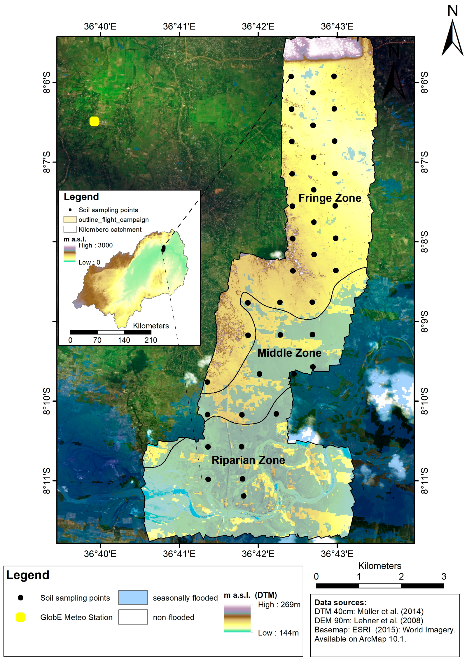
2.1. Study Area

The study area is a confined wetland transect located in the north of the Kilombero floodplain between latitude 7.67°–10.03° S and longitude 34.56°–37.29° E in the Morogoro region in Southern Tanzania (Figure 1). The Kilombero catchment comprises 40,240 km² covering the broad floodplain of the main Kilombero River [17]. The floodplain is framed by the Northwestern Udzungwa mountains and the Mahenge and Mbarika mountains in the southeast with elevation ranges between 200 and 2500 m above sea level (m a.s.l.) [27]. Geologically, the plain is characterized by sedimentary basin infillings forming a seasonal alluvial floodplain dominated by Fluvisols [28]. The Kilombero catchment receives a bimodal pattern of rainfall which is mainly driven by the movement of the Intertropical Convergence Zone (ITCZ). The annual rainfall ranges from 1200–1400 mm with a mean annual temperature of about 23–25 °C [29]. Short rains are experienced in the months of November to January, and long rains occur between March and May of every year. A dry spell is experienced between the months of June and November annually [29,30,31]. According to the annual rainfall pattern, the Kilombero River floodplain is prevailingly flooded during the long rainy season. The main cultivated crops are rice and cash-crops such as maize and sugarcane by large- and small-scale farmers. Additionally, land use systems comprise of fishery and cattle grazing [32]. The predominant semi-natural vegetation of the floodplain comprises of 1–3 m high Guinea grass (Panicum maximum L.), Pennisetum sp. grasses and some small areas of flood resistant woodlands consisting of Kigeliapinnata, Lonchocarpuscapassa, and Combretum sp.

2.2. Experimental Design

For the analysis of the spatial distribution of the selected soil properties in the floodplain, soil sampling was conducted at three hydrological zones: fringe, middle, and riparian (Figure 1). The hydrological zones were subdivided based on origin, extent, duration, and depth of flooding water. The fringe zone is characterized by precipitation and ground water induced flooding and a balanced groundwater table dynamic with shallow depth inundation [33]. Landsat 7 ETM+ and 8 OLI surface reflectance images [34,35] were processed to identify riverine flooded areas and generate inundation extents for seasonally-flooded sections during the long rainy season (Figure 1). The non-flooded part was defined as fringe zone. The middle zone is partially flooded, whereas the riparian zone is nearly completely flooded during the long rainy season. Additionally, the flooding depth and duration are higher and longer, respectively in the riparian zone. The spatial differentiation between these two riverine flooded hydrological zones was applied by a combination of two remote sensing products and the following three boundary conditions. The first boundary condition for the riparian area was an effectively full coverage of the seasonal flooding detected by Landsat images. The second boundary condition was the absolute distance to the river and the third boundary condition was the absolute height derived from the Digital Elevation Mode (DEM) as a proxy for the inundation depths and lengths. The lower parts of transect were assumed to be flooded more deeply and hence for a longer period. Overall, the riparian zone is close to the river, low in absolute altitude, and nearly completely flooded, while the middle zone still has greater shares of non-flooded areas and more shallowly inundated areas.

2.3. Soil Sampling and Analysis

Disturbed and undisturbed (100 cm³) soil samples were taken from 0–20 cm (topsoil) and 20–40 cm (subsoil) in a regular grid design. Due to the size and shape of each hydrological zone the number of sampling spots varied from 20 (fringe, trigonal design) to 9 (middle and riparian, rectangular design). Each sampling spot was not more than 750 m away from the next. The undisturbed soil samples were analyzed for bulk density using the core method. Disturbed samples were air-dried, and ground to pass through a 2-mm sieve prior to the analysis of soil organic carbon (SOC) and soil texture. SOC was determined using a modified Walkley-Black-method [36], and soil texture was determined using the laser method (LA950, Horiba Instruments Inc., Irvine, CA, USA) [37] following the technical procedure protocol [38]. Additionally, undisturbed (250 cm³) soil samples were taken from 17 spots at four depths (10, 20, 30, and 40 cm) to determine the saturated hydraulic conductivity using a laboratory permeameter (Eijkelkamp, Griesbeek, Netherlands) [39] following the procedures described by Eijkelkamp [39]. Analysis was performed in duplicate. All sampling took place in March and April 2015.

2.4. Soil Moisture Monitoring

To understand the spatial distribution of soil moisture content along the hydrological zones of the floodplain, measurements were conducted using frequency domain reflectometry (FDR) profile probe type PR2 [40] equipped with HH2 moisture meter (Dynamax Inc., Houston, TX, USA) [41] at depths of 10, 20, 30, and 40 cm. A total of 17 access tubes were installed at each hydrological zone. Soil moisture was monitored every two days for a period of eighteen months (March 2015–August 2016) except during periods when the wetland was flooded or probe failure.

2.5. Statistical and Spatial Analysis

Statistical analysis of data involved two approaches; classical statistical analysis, and geostatistical analysis to establish spatial patterns of soil properties.

2.5.1. Classical Statistical Analysis

To ascertain patterns and trends in data, descriptive statistics covering mean, standard deviation (SD), median and coefficient of variation (CV) were computed for each soil property and soil moisture. CVs were expressed according to Wilding [42]; CV < 15% signifies low variability, CV < 35% signifies moderate variability, CV > 35% signifies high variability. Significance in mean differences related to hydrological zones and soil depths were tested using analysis of variance (ANOVA). Significance difference between means in the ANOVA test was determined at p < 0.05. Classical statistical analysis was conducted with the STATA statistical package.

2.5.2. Geostatistical Spatial Analysis

Geostatistical analysis was applied to detect and map spatial distribution of selected soil physical properties (SOC, Bulk density, and texture). Geostatistical analysis involved the kriging method [43]. Kriging interpolates data of non-sampled point locations on the basis of sampled locations [44]. Spatial autocorrelation determines interrelation of the values and analysis of existence of a spatial pattern. A function is fitted to a number of points within a specified radius to determine values of unmeasured points. Ordinary kriging assumes there is no trend that is, constant mean over the areal mean [45]. Ordinary kriging in ArcGIS 10.3.1 was adopted to generate raster images. The semivariograms were generated with the Geostatistical Analyst toolbox and the models used in kriging.

Variograms express the spatial variance of data points:

$$\mathbf{\gamma }\left(\mathit{h}\right)=\frac{1}{2\mathit{N}\left(\mathit{h}\right)}{\displaystyle \sum }_i^{\mathit{N}\left(\mathit{h}\right)}[{\left(\mathit{z}\left({\mathit{x}}_{\mathit{i}}\right)-\mathit{z}\left({\mathit{x}}_{\mathit{i}}+\mathit{h}\right)\right)}^2]$$

(1)

where $\mathbf{\gamma }\left(\mathit{h}\right)$ is the semi variance between all observations, $\mathit{N}\left(\mathit{h}\right)$ is the number of pairs of observations separated by distance $\mathit{h}$, $\mathit{z}\left({\mathit{x}}_{\mathit{i}}\right)$ is the measured soil moisture value at the sample point ${\mathit{x}}_{\mathit{i}}$ and $\mathit{z}\left({\mathit{x}}_{\mathit{i}}+\mathit{h}\right)$ is the measured soil moisture value at location ${\mathit{x}}_{\mathit{i}}+\mathit{h}$.

The exponential variogram is given by:

$$\mathbf{\gamma }\left(\mathit{h}\right)=\{\begin{array}{c}0\\ \mathit{C}\mathbf{0}+\mathit{C}\mathbf{1}(1-e^{\raisebox{1ex}{$-h$}\!\left/ \!\raisebox{-1ex}{$a$}\right.})\end{array}\begin{array}{c}h=0\\ h>0\end{array}$$

(2)

where $\mathit{C}\mathbf{0}$ is the nugget variance, $\mathit{C}\mathbf{1}$ is the structural variance (C ≥ C0), $\mathit{C}\mathbf{0}+\mathit{C}\mathbf{1}$ is the sill, and a is the range.

Variation due to random factors is given by nugget variance. The sill gives a variation due to the structure of the data. The range gives the distance over which the data points are correlated. Spatial dependence is computed as the ratio of nugget to sill. Strong spatial dependence is lower than 25%; a ratio greater than 75% indicates low spatial dependence and values between 25% and 75% moderate dependence [46]:

$$degreeofspatialdependence=\frac{\mathit{C}\mathbf{0}}{\mathit{C}\mathbf{0}+\mathit{C}\mathbf{1}}\times \mathbf{100}\%$$

(3)

where $\mathit{C}\mathbf{0}$ is the nugget variance, $\mathit{C}\mathbf{1}$ the structural variance, $\mathit{C}\mathbf{0}+\mathit{C}\mathbf{1}$ is the sill, and a is the range.

3. Results

3.1. Variability of Selected Soil Properties

The descriptive statistical analysis of the total soil sample quantity of the selected floodplain transect (

Table 1. Descriptive statistics of selected soil properties within the entire floodplain transect.

Soil Property	n	Mean	SD	Min	Max	Median	CV (%)
BD (g∙cm−3)	76	1.38	0.13	1.00	1.70	1.39	9.70
SOC (g∙kg−1)	76	11.1	5.2	1.40	25.7	10.8	47.04
Ksat (cm∙d−1)	76	41.73	64.75	4.00	478.2	25.66	155.2
Sand (%)	76	27.10	20.61	1.04	72.21	26.66	76.05
Silt (%)	76	53.71	13.09	25.96	74.28	55.94	24.37
Clay (%)	76	19.19	11.62	1.17	47.27	14.40	60.55

BD: Bulk density; SOC: Soil Organic Carbon; K_sat: Saturated hydraulic conductivity; SD: Standard deviation; CV: Coefficient of variation; n: Number of samples.

) described a general low variability of the bulk density with a coefficient of variation (CV) of 9.7%, and an overall mean of 1.38 g∙cm³. The silt had a CV of 24.4%, indicating a moderate variability with an overall mean of 53.7%. All other soil physical variables were characterized by a high variability with a CV ranging from 47.0% for soil organic carbon (SOC) up to 155.2% for saturated hydraulic conductivity (K_sat). This was also expressed for each soil physical variable with a high and accordingly moderate and low standard deviation (SD) with respect to the particular mean value.

3.2. Spatial Variability of Selected Soil Properties Across the Hydrological Zones

Table 2. Spatial variability of mean values of selected soil properties for the three defined hydrological zones at 0–20 cm and 20–40 cm depths.

Soil Depth	Hydrological Zone	n	BD (g∙cm−3)	SOC (g∙kg−1)	Ksat (cm∙d−1)	Sand (%)	Silt (%)	Clay (%)
0–20 cm	Riparian	9	1.26	10.9	68.2	27	53.8	19.2
	Middle	9	1.31	12	29.8	14.1	59.3	26.6
	Fringe	20	1.41	13	27.9	33.7	52	14.3
20–40 cm	Riparian	9	1.31	9.4	70.1	20.7	58	21.3
	Middle	9	1.43	10.4	35	12.4	56.9	30.8
	Fringe	20	1.46	10.1	39.3	35.9	49.5	14.6
p-value (depth)			0.016	NS	NS	NS	NS	NS
p-value (hydrologic zones)			<0.001	NS	NS	<0.001	NS	<0.001

BD: Bulk density; SOC: Soil Organic Carbon; K_sat: Saturated hydraulic conductivity; n: Number of samples; NS: Not significant at p < 0.05.

shows the spatial variability of selected soil physical properties along the defined hydrological zones of the floodplain transect. The bulk density of the topsoil ranges from 1.0–1.6 g∙cm⁻³ and was highest in the fringe zone (mean = 1.41 g∙cm⁻³), followed by the middle (mean = 1.31 g∙cm⁻³), and riparian zones (mean = 1.26 g∙cm⁻³). The subsoil had the highest bulk density in the fringe zone (mean = 1.46 g∙cm⁻³) followed by the middle (mean = 1.43 g∙cm⁻³) and riparian zones (mean = 1.31 g∙cm⁻³). The calculated p-value for the bulk density variable indicated a significant difference for bulk density by depth (p = 0.016) and hydrological zone (p < 0.01). For the other soil physical variables a significant difference was observed for the soil texture fraction by hydrological zone for sand and clay. The remaining variables were not significantly different across depths or hydrological zones.

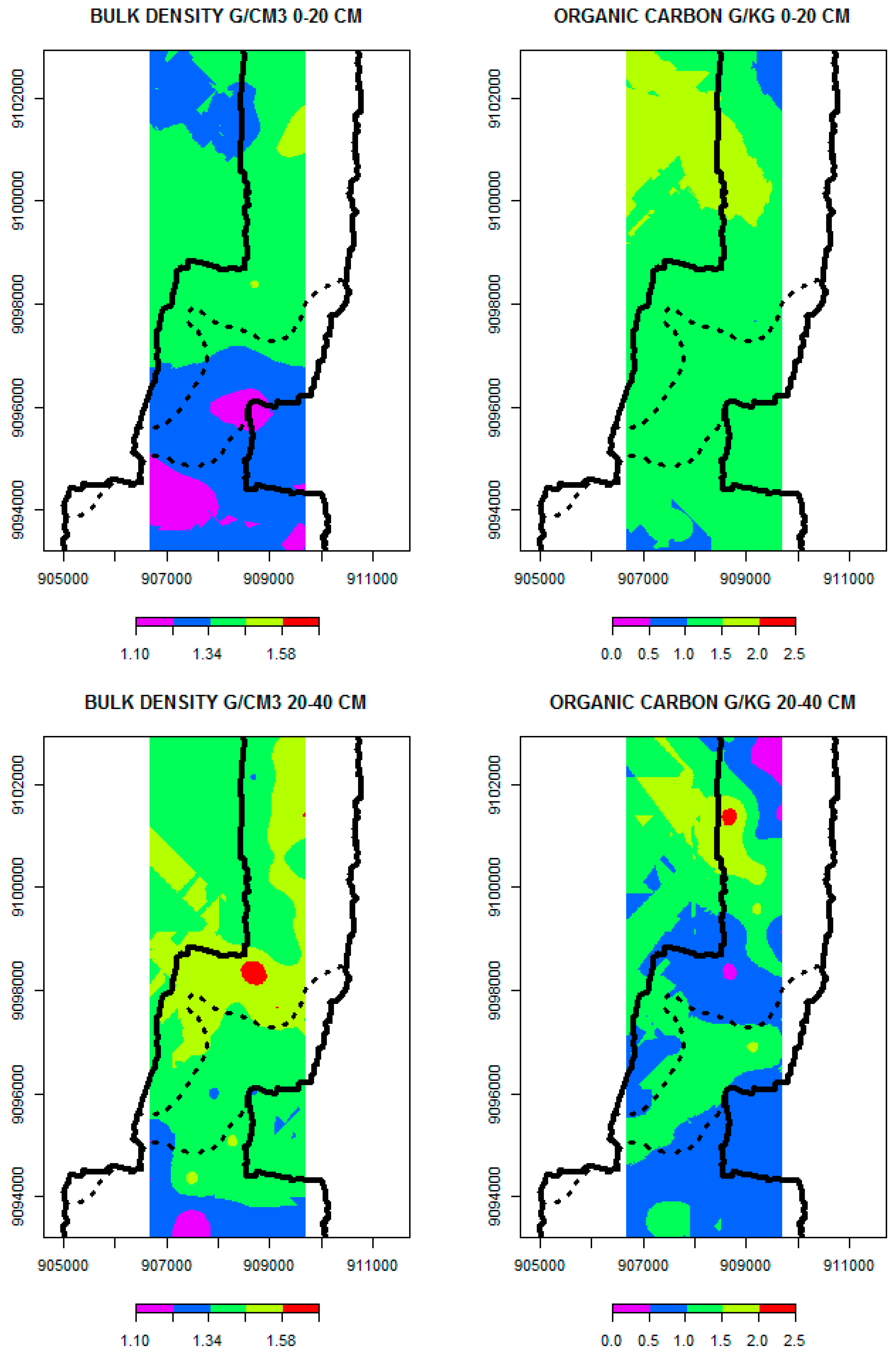
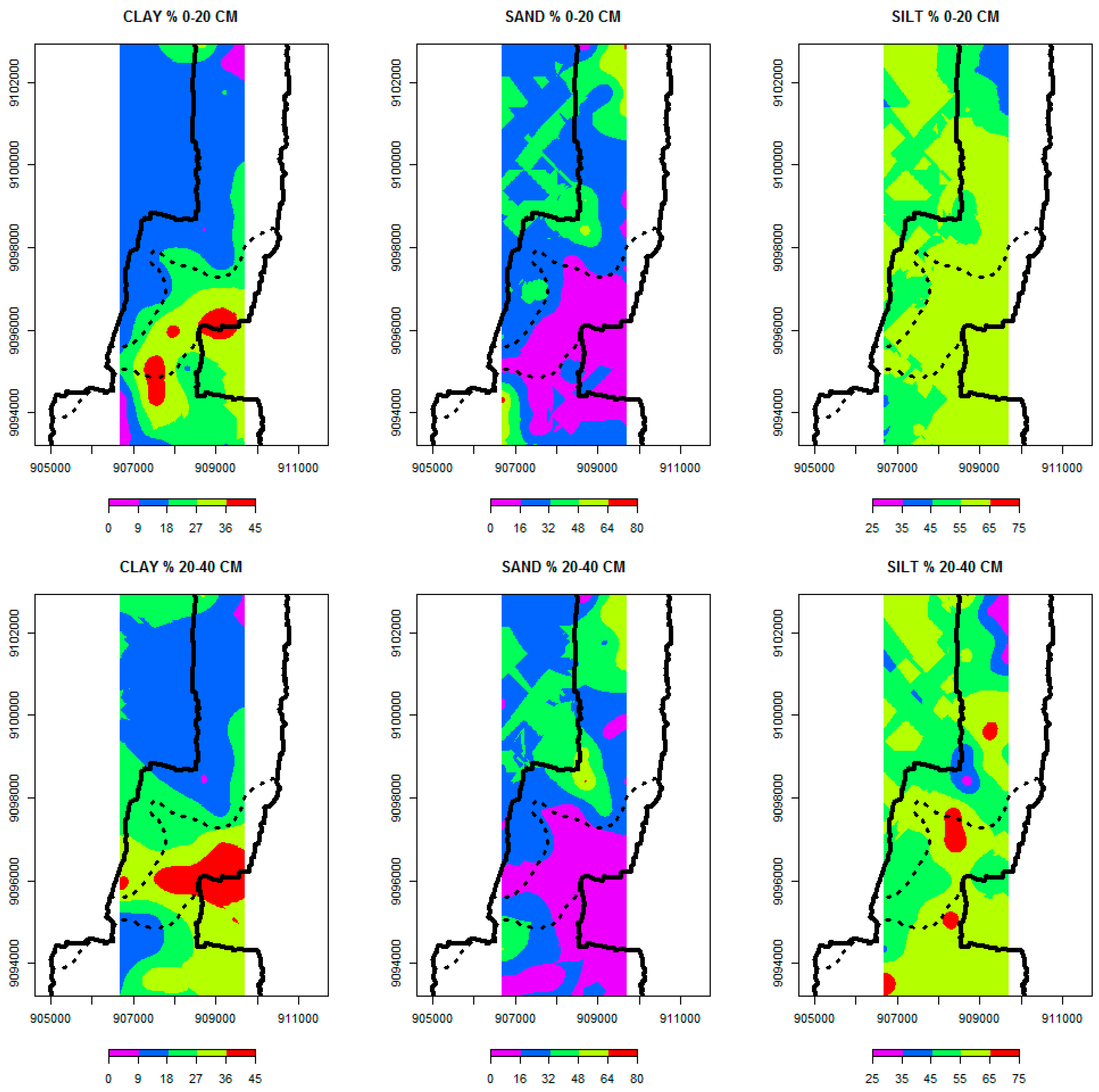
3.3. Geostatistical Analysis of Soil Physical Properties

The images showing spatial variation of soil properties derived from the geostatistical kriging method are presented in Figure 2 and Figure 3. The results indicate that the bulk density, silt, and organic carbon at 0–20 cm had intermediate dependence, whereas all the other soil parameters at 0–20 cm and 20–40 cm depth had high spatial dependence. Images generated at a depth of 20–40 cm had lower RMSE errors as compared to their corresponding image at depths of 0–20 cm for all parameters except clay (

Table 3. Summary of model parameters fitted through the semi-variograms for all sample points in the floodplain.

Soil Property	Depth (cm)	Model	Lag Size	Nugget (C0)	Range	Partial Sill (C)	Spatial Dependence (C0/C0 + C) × 100	RMSE
BD (g∙cm−3)	0–20	Exp	204.16	0.01	2449.97	0.01	43.36	0.12
	20–40	Exp	156.68	0.00	1277.13	0.01	0.00	0.11
Silt (%)	0–20	Exp	157.72	95.54	1244.62	80.99	54.12	13.95
	20–40	Exp	159.83	0.00	1463.32	175.80	0.00	12.39
Clay (%)	0–20	Exp	442.81	0.00	2815.90	138.76	0.00	9.88
	20–40	Exp	649.99	15.25	5568.68	170.29	8.22	10.26
Sand (%)	0–20	Exp	158.77	0.00	1244.62	409.47	0.00	20.70
	20–40	Exp	202.82	0.00	1984.02	377.72	0.00	17.28
SOC (g∙kg−1)	0–20	Exp	280.49	0.20	3365.94	0.12	62.47	0.52
	20–40	Exp	168.51	0.00	1273.26	0.29	0.00	0.48

).

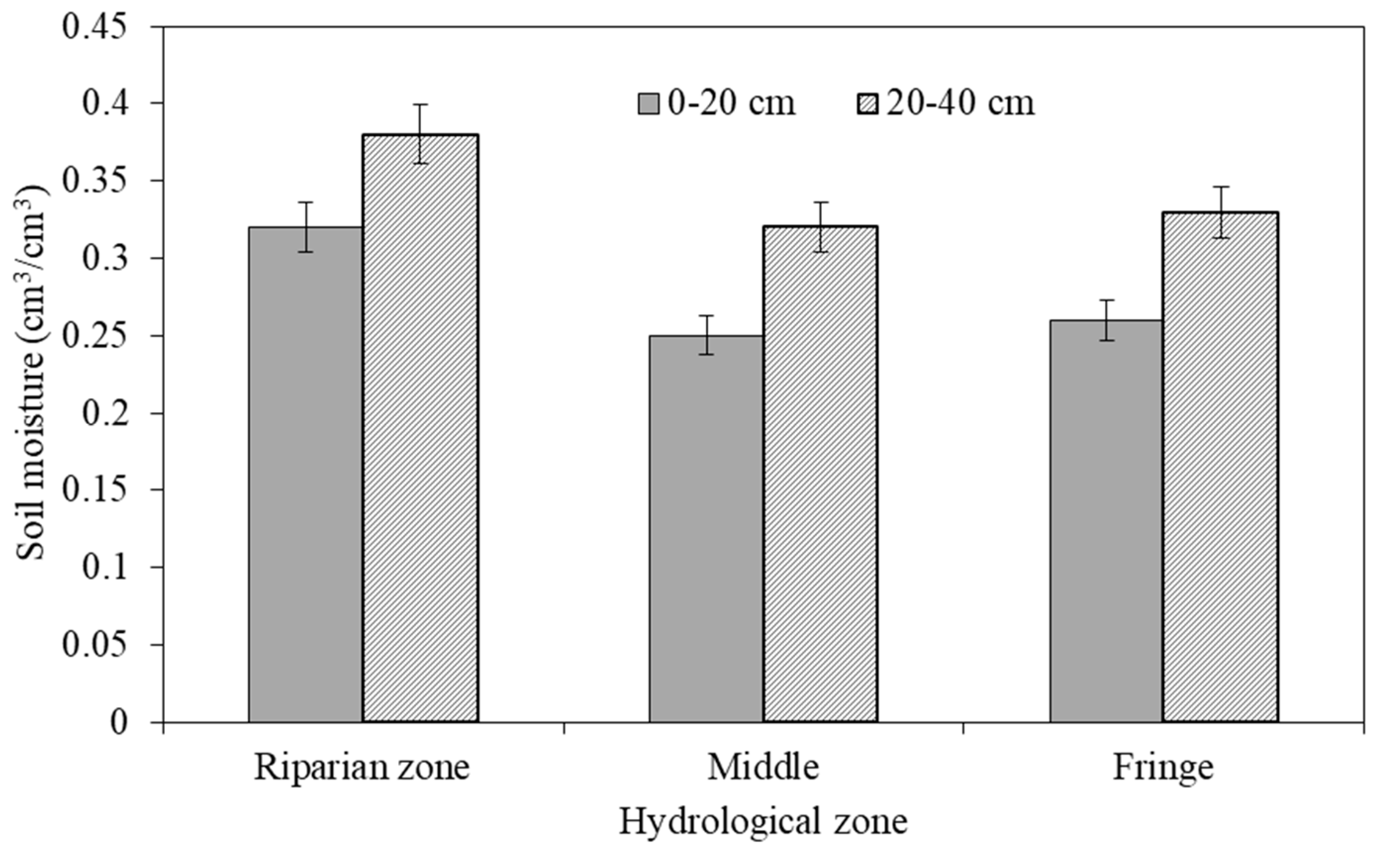
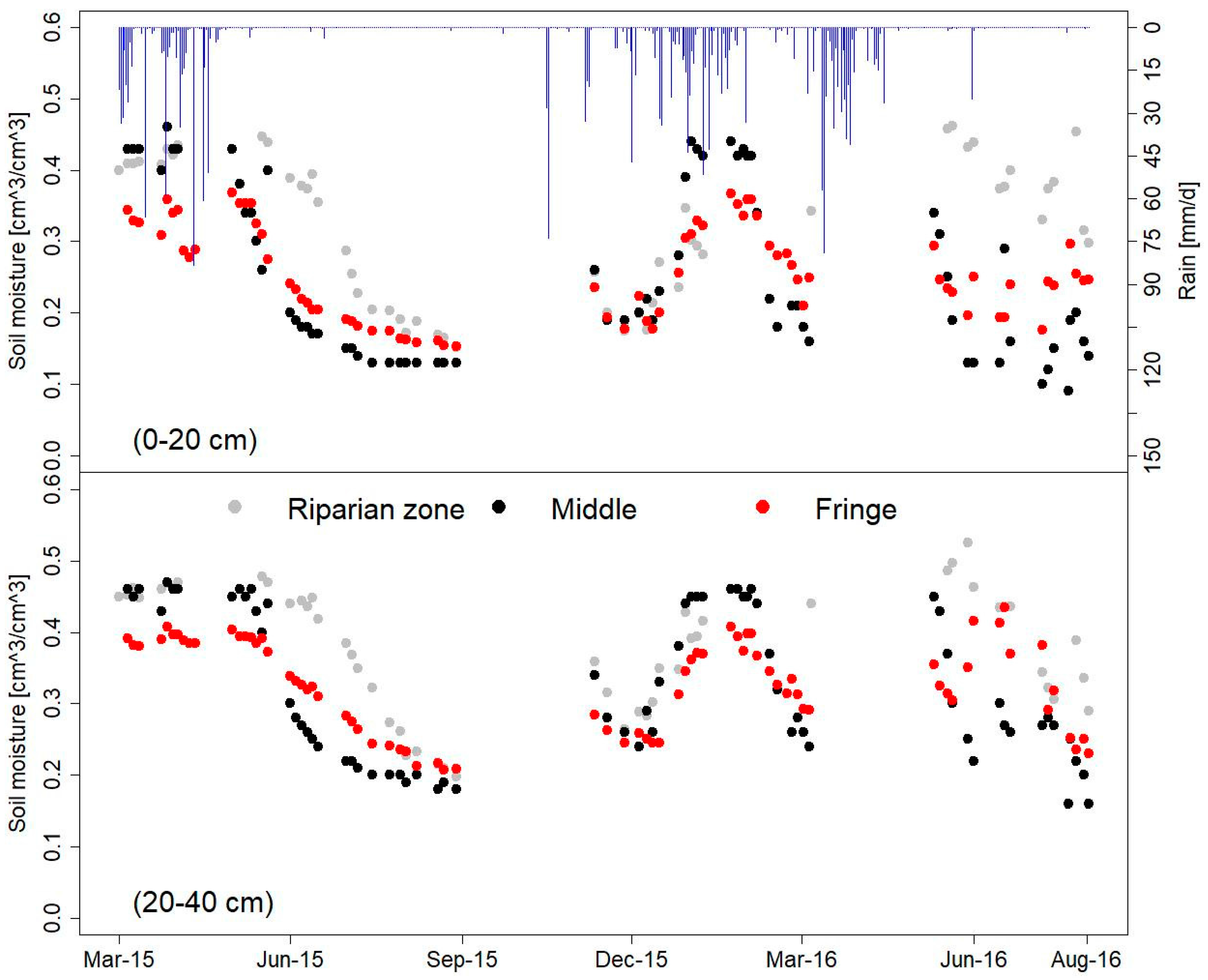
3.4. Spatial and Temporal Soil Moisture Variability

The spatial analysis of soil moisture measurements according to the hydrological zones and depths showed a higher soil moisture at the subsoil (20–40 cm) compared to the topsoil (0–20 cm) layer along all hydrological zones (Figure 4). There was a significant (p < 0.05) difference in soil moisture content across the hydrological zones and soil depth. The riparian zone retained the highest soil moisture content for all the depths compared to the middle and fringe zones. The temporal pattern of soil moisture dynamics along the hydrological zones (Figure 5) corresponded to rainfall seasonality of the Kilombero floodplain with a long dry season from June to November, a short rainy season from December to January, and a long rainy season from March to May. Furthermore, the temporal dynamics showed that in comparison to the middle and fringe zones, the riparian zone retained the saturated soil moisture content for a longer period of time describing a convex shape of the sloping curve of soil moisture content for both soil layers. The soil moisture time series of the middle and fringe zones described a concave sloping curve for the topsoil and for the middle zone in the subsoil. Overall, the saturated soil moisture at the riparian and middle zones showed higher values than the fringe zone.

4. Discussion

The soils depicted high spatial variability with a CV above 35%, especially percentage clay and sand, SOC and Ksat across the hydrological zones of the floodplain. Soil properties depicting low variability with CVs below 35% were bulk density and silt. The high variability is not unusual for cultivated floodplain environments. The spatial variability may emanate from nature of parent materials, climate, flora, fauna, land use, management practices [47], and deposition of materials from flooding due to river overbank flow. The results also showed that the bulk density increased with depth and it was higher in the subsoil and in the fringe zone. The increase of bulk density in the subsoil was most likely due to soil compaction and resulting in decreasing soil porosity. Furthermore, the increasing bulk density correlates with increasing distance from river, related with inundation depth, duration and frequency. The bulk density is reported to increase with compaction and with increasing depth [48]. The literature shows that human activities, like frequent farming, tend to increase soil compaction and, hence, increase the bulk density [49]. Further studies show that floods cause fluvial deposits rich in organic matter, also increasing the bulk density. Other studies demonstrated that bulk density is the soil hydraulic property that influences soil water movement and retention [50]. In this study we observed bulk densities ranging from 1.0 g∙cm⁻³ to 1.70 g∙cm⁻³. Other researchers have reported that bulk densities of less than 1.5 g∙cm⁻³ are good for agricultural activities because it allows for optimum movement of water and air [51]. It is reported by [52] that soils with a bulk density higher than 1.6 g∙cm⁻³ tend to restrict root growth. This interferes with the ability of the plant to absorb water and nutrients.

The SOC distribution showed higher values in the topsoil in all three hydrological zones than in the subsoil. The results of SOC obtained in all three hydrological zones was comparably lower than the threshold of 3% recommended for agricultural tropical soils. Below this value, SOC is insufficient in quantity and possesses potential negative effects on the quality of arable land [53]. Though it affects the rate of decomposition of organic matter, the amount of carbon and nitrogen is an important factor in agricultural activities [54]. The binding capacity of organic matter creates higher soil porosity and reduced soil bulk density [55]. The observed low values of SOC in all three hydrological zones of the floodplain could be attributed to the high silt and sand content, and common management practices in the floodplain, like bush burning for field preparation. Additionally, the low organic carbon content could be related to minor vegetation growth and fast rate of decomposition under high temperature during the dry season.

This study observed variations in silt, clay, and sand soil textures. Silty soil was dominant in all hydrological zones, whereas sand and clay described a significant difference in the classical statistical analysis (Table 2) which is also reflected in the geostatistical spatial analysis (Figure 3). The observed variations might be due to sedimentary variations rather than soil forming processes, nature of parent materials, and the energy of deposition of the river. The soil texture is an important parameter in agriculture as it is related to soil aeration, soil water supply, the cation-exchange capacity, and soil hydraulic conductivity [56]. There was no significant variation in hydraulic conductivity in all three hydrological zones. Hydraulic conductivity is associated with soil types, land uses, positions on landscape, preferential flow, depths, instruments, and methods of measurement and experimental errors [47]. During data collection the samples were collected at different hydrological zones approximately 1 km apart (Figure 1), but there was no statistically significant variation in hydraulic conductivity in the fringe, middle and riparian zones. Moreover, hydraulic conductivity might be affected by additional factors such as vegetation cover, bio- and human activities [57]. The overall all-season lower soil moisture values of the middle and fringe zones were related to the global variability of the soil physical properties bulk density and soil texture, resulting in a common lower saturated soil water content with respect to hydrological zones. Additionally, soil management practices like tillage, have an impact on soil physical properties and, hence, on overall soil moisture content [58,59]. Though the riparian zone was characterized by the deepest and longest inundation of the floodplain, this was also reflected in the soil moisture dynamics at the beginning of the dry season retrieving soil moisture for a longer period, which is reflected in a convex shape of the soil moisture sloping curve at the start of the dry season.

5. Conclusions

The study shows that soil properties in the Kilombero floodplain are generally heterogeneous and spatially variable. Noteworthy is that quantities of SOC, K_sat, and silt content were not significantly different among the three defined hydrological zones. The spatial dependence of soil properties in the floodplain is generally high. The results also show that spatial soil moisture content increases towards the Riparian zone. The riparian zone retains relatively high temporal soil moisture content for longer periods of time, which exhibits a convex shape of the soil moisture slope curve at the start of the dry season, whereas a concave sloping curve for soil moisture time series is exhibited at the middle and fringe zones.

References

1. Sun, B.; Zhou, S.; Zhao, Q. Evaluation of spatial and temporal changes of soil quality based on geostatistical analysis in the hill region of subtropical China. Geoderma 2003, 115, 85–99. [Google Scholar] [CrossRef]
2. Gonzales, O.J.; Zak, D.R. Geostatistical analysis of soil properties in a secondary tropical dry forest, St. Lucia, West Indies. Plant Soil 1994, 163, 45–54. [Google Scholar] [CrossRef]
3. Adhikari, K.; Guadagnini, A.; Toth, G.; Hermann, T. Geostatistical analysis of surface soil texture from Zala County in western Hungary. In Proceedings of the International Symposium on Environment, Energy and Water in Nepal: Recent Researches and Direction for Future, Kathmandu, Nepal, 31 March–1 April 2009; pp. 219–224. [Google Scholar]
4. Abuduwaili, J.; Tang, Y.; Abulimiti, M.; Liu, D.; Ma, L. Spatial distribution of soil moisture, salinity and organic matter in Manas River watershed, Xinjiang, China. J. Arid Land 2012, 4, 441–449. [Google Scholar] [CrossRef]
5. Hupet, F.; Vanclooster, M. Intraseasonal dynamics of soil moisture variability within a small agricultural maize cropped field. J. Hydrol. 2002, 261, 86–101. [Google Scholar] [CrossRef]
6. Lal, R.; Shukla, M.K. Principles of Soil Physics; Dekker Inc.: New York, NY, USA, 2004; ISBN 0-8247-5324-0. [Google Scholar]
7. Crave, A.; Gascuel-Odoux, C. The influence of topography on time and space distribution of soil surface water content. Hydrol. Process. 1997, 11, 203–210. [Google Scholar] [CrossRef]
8. Ngailo, J.A.; Vieira, S.R. Spatial patterns and correlation of soil properties of a lowland soil. J. Soil Sci. Environ. Manag. 2012, 3, 287–296. [Google Scholar] [CrossRef]
9. Iqbal, J. Spatial Variability Analysis of Soil Physical Properties of Alluvial Soils. Soil Sci. Soc. Am. J. 2005, 69, 1338–1350. [Google Scholar] [CrossRef]
10. Banta, S.; Mendoza, C.V. Organic Matter and Rice; International Rice Institute: Los Banos Laguna, Phillipines, 1984; ISBN 971-104-104-9. [Google Scholar]
11. Reddy, K.R.; DeLaune, R.D. Biogeochemistry of Wetlands: Science and Applications; Taylor and Francis GRoup: Boca Raton, FL, USA, 2008. [Google Scholar]
12. Wendroth, O.; Reynolds, D.; Vieira, S.; Reichardt, K.; Wirth, S. Statistical approaches to the analysis of soil quality data. In Soil Quality for Crop Production and Ecosystem Health; Elsevier: Amsterdam, The Netherlands, 1997; pp. 247–276. [Google Scholar]
13. Santra, P.; Chopra, U.K.; Chakraborty, D. Spatial variability of soil properties and its application in predicting surface map of hydraulic parameters in an agricultural farm. Curr. Sci. 2008, 95, 937–945. [Google Scholar]
14. Reza, S.K.; Sarkar, D.; Baruah, U.; Das, T.H. Evaluation and comparison of ordinary kriging and inverse distance weighting methods for prediction of spatial variability of some chemical parameters of Dhalai district, Tripura. Agropedology 2010, 20, 38–48. [Google Scholar]
15. Elbasiouny, H.; Abowaly, M.; Abu_Alkheir, A.; Gad, A. Spatial variation of soil carbon and nitrogen pools by using ordinary Kriging method in an area of North Nile Delta, Egypt. CATENA 2014, 113, 70–78. [Google Scholar] [CrossRef]
16. Xu, X.; Kalhoro, S.A.; Chen, W.; Raza, S. The evaluation/application of Hydrus-2D model for simulating macro-pores flow in loess soil. Int. Soil Water Conserv. Res. 2017, 5, 196–201. [Google Scholar] [CrossRef]
17. Cornelissen, T.; Diekkrüger, B.; Giertz, S. A comparison of hydrological models for assessing the impact of land use and climate change on discharge in a tropical catchment. J. Hydrol. 2013, 498, 221–236. [Google Scholar] [CrossRef]
18. Mango, L.M.; Melesse, A.M.; McClain, M.E.; Gann, D.; Setegn, S.G. Land use and climate change impacts on the hydrology of the upper Mara River Basin, Kenya: Results of a modeling study to support better resource management. Hydrol. Earth Syst. Sci. 2011, 15, 2245–2258. [Google Scholar] [CrossRef]
19. Yira, Y.; Diekkrüger, B.; Steup, G.; Bossa, A.Y. Impact of climate change on hydrological conditions in a tropical West African catchment using an ensemble of climate simulations. Hydrol. Earth Syst. Sci. 2017, 2143–2161. [Google Scholar] [CrossRef]
20. Bormann, H.; Breuer, L.; Gräff, T.; Huisman, J.A. Analysing the effects of soil properties changes associated with land use changes on the simulated water balance: A comparison of three hydrological catchment models for scenario analysis. Ecol. Model. 2007, 209, 29–40. [Google Scholar] [CrossRef]
21. Montzka, C.; Moradkhani, H.; Weihermüller, L.; Franssen, H.J.H.; Canty, M.; Vereecken, H. Hydraulic parameter estimation by remotely-sensed top soil moisture observations with the particle filter. J. Hydrol. 2011, 399, 410–421. [Google Scholar] [CrossRef]
22. Yang, X. Evaluation and application of DRAINMOD in an Australian sugarcane field. Agric. Water Manag. 2008, 95, 439–446. [Google Scholar] [CrossRef]
23. Danvi, A.; Giertz, S.; Zwart, S.J.; Diekkrüger, B. Comparing water quantity and quality in three inland valley watersheds with different levels of agricultural development in central Benin. Agric. Water Manag. 2017, 192, 257–270. [Google Scholar] [CrossRef]
24. Yang, H.; Wang, H.; Fu, G.; Yan, H.; Zhao, P.; Ma, M. A modified soil water deficit index (MSWDI) for agricultural drought monitoring: Case study of Songnen Plain, China. Agric. Water Manag. 2017, 194, 125–138. [Google Scholar] [CrossRef]
25. Mombo, F.; Speelman, S.; Van Huylenbroeck, G.; Hella, J.; Moe, S. Ratification of the Ramsar convention and sustainable wetlands management: Situation analysis of the Kilombero Valley wetlands in Tanzania. J. Agric. Ext. Rural Dev. 2011, 3, 153–164. [Google Scholar]
26. Rebelo, L.-M.; McCartney, M.P.; Finlayson, C.M. Wetlands of Sub-Saharan Africa: Distribution and contribution of agriculture to livelihoods. Wetl. Ecol. Manag. 2010, 18, 557–572. [Google Scholar] [CrossRef]
27. Leemhuis, C.; Thonfeld, F.; Näschen, K.; Steinbach, S.; Muro, J.; Strauch, A.; López, A.; Daconto, G.; Games, I.; Diekkrüger, B. Sustainability in the food-water-ecosystem nexus: The role of land use and land cover change for water resources and ecosystems in the Kilombero Wetland, Tanzania. Sustainability 2017, 9. [Google Scholar] [CrossRef]
28. Beck, A.D. The Kilombero valley of south-central Tanganyika. East Afr. Geogr. Rev. 1964, 1964, 37–43. [Google Scholar]
29. Koutsouris, A.J.; Chen, D.; Lyon, S.W. Comparing global precipitation data sets in Eastern Africa: A case study of Kilombero Valley, Tanzania. Int. J. Climatol. 2016, 36, 2000–2014. [Google Scholar] [CrossRef]
30. Nicholson, S.E. A review of climate dynamics and climate variability in Eastern Africa. In The Limnology, Climatology and Paleoclimatology of the East African Lakes; Gordon and Breach: Amsterdam, The Netherlands, 1996; pp. 25–26. [Google Scholar]
31. Basalirwa, C.P.K.; Odiyo, J.O.; Mngodo, R.J.; Mpeta, E.J. The climatological regions of Tanzania based on the rainfall characteristics. Int. J. Climatol. 1999, 19, 69–80. [Google Scholar] [CrossRef]
32. Hughes, R.H.; Hughes, J.S. A Directory of African Wetlands; IUCN: Gland, Switzerland, 1992; ISBN 978-2-88032-949-5. [Google Scholar]
33. Burghof, S.; Gabiri, G.; Stumpp, C.; Chesnaux, R.; Reichert, B. Development of a hydrogeological conceptual wetland model in the data-scarce North-Eastern region of Kilombero Valley, Tanzania. Hydrogeol. J. 2017. [Google Scholar] [CrossRef]
34. Department of the Interior, U.S.G.S. Product Guide—Landsat 4–7 Surface Reflectance (LEDAPS) Product Version 8.0. Available online: https://landsat.usgs.gov/sites/default/files/documents/ledaps_product_guide.pdf (accessed on 6 August 2017).
35. Department of the Interior, U.S.G.S. Product Guide Landsat 8 Surface Reflectance Code (LASRC) Product Version 4.1. Available online: https://landsat.usgs.gov/sites/default/files/documents/lasrc_product_guide.pdf (accessed on 6 August 2017).
36. Okalebo, J.; Gathua, K.; Woomer, P. Laboratory Methods of Plant and Soil Analysis: A Working Manual; Tropical Soil Biology and Fertility Programme: Nairobi, Kenya, 2002. [Google Scholar]
37. Horiba Instruments Inc.; Irvine, U. LA950. Available online: http://www.horiba.com/fileadmin/uploads/Scientific/Documents/PSA/LA950_V2_bro.pdf (accessed on 27 November 2017).
38. Horiba, S. A Guidebook to Particle Size Analysis. Available online: www.horiba.com/us/particle (accessed on 20 May 2015).
39. Eijkelkamp User Manual. Available online: https://en.eijkelkamp.com/products/laboratory-equipment/soil-water-permeameters.html (accessed on 27 November 2017).
40. Delta-T Devices Ltd. User Manual for the Profile Probe Type PR2. Available online: ftp://ftp.dynamax.com/manuals/PR2_QSG.pdf (accessed on 3 March 2014).
41. Delta-T Devices Ltd. User Manual for the Moisture Meter Type HH2. Available online: http://www.delta-t.co.uk/wp-content/uploads/2016/10/HH2-UM-4.2.pdf (accessed on 3 March 2014).
42. Wilding, L.G. Soil spatial variability: Its documentation, accommodation and implication to soil surveys. In Soil Spatial Variability Proceedings of a Workshop of the ISSS and the SSA, Las Vegas PUDOC, Wageningen; Center Agricultural Pub and Document, Pudoc Wageningen: Wageningen, The Netherlands, 1985; pp. 166–187. [Google Scholar]
43. Webster, R.; Oliver, M.A. Geostatistics for Environmental Scientists, 2nd ed.; Wiley: Chichester, UK, 2007; ISBN 978-0-470-02858-2. [Google Scholar]
44. Hengl, T. A Practical Guide to Geostatistical Mapping, 2nd ed.; Hengl: Amsterdam, The Netherlands, 2009; ISBN 978-90-90-24981-0. [Google Scholar]
45. Childs, C. Interpolating surfaces in ArcGIS spatial analyst. ArcUser Jul.–Sept. 2004, 3235, 569. [Google Scholar]
46. Huang, Y.; Wang, Y.; Zhao, Y.; Xu, X.; Zhang, J.; Li, C. Spatiotemporal distribution of soil moisture and salinity in the taklimakan desert highway shelterbelt. Water (Switzerland) 2015, 7, 4343–4361. [Google Scholar] [CrossRef]
47. Stockton, J.; Warrick, A. Spatial variability of unsaturated hydaulic conductivity. Soil Sci. Soc. Am. J. 1971, 35, 201–205. [Google Scholar] [CrossRef]
48. Arshad, M.A.; Martin, S. Identifying Critical Limits for Soil Quality Indicators in Agro-Ecosystem. Agric. Ecosyst. Environ. 2002, 88, 153–160. [Google Scholar] [CrossRef]
49. Maurice, K.; Boniface, O.; Francis, P. Intensity of Farmland Cultivated and Soil Bulk Density in Different Physiographic Units in Nyakach District. IOSR J. humanit. Soc. Sci. 2014, 19, 86–91. [Google Scholar]
50. Rawls, W.J. Estimating soil bulk density from particle size analysis and organic matter content. Soil Sci. 1983, 135, 123–125. [Google Scholar] [CrossRef]
51. Hunt, N.; Gilkes, B. Farm Monitoring Handbook; University of Western Australia, Land Management Society, and National Dryland Salinity Program: Crawley, Australia, 1992. [Google Scholar]
52. McKenzie, N.; Coughlan, K.; Cresswell, H. Soil Physical Measurement and Interpretation for Land Evaluation; CSIRO Publishing: Clayton, Australia, 1992; Volume 5, ISBN 9780643069879. [Google Scholar]
53. Loveland, P.; Webb, J. Is there a critical level of organic matter in the agricultural soils of temperate regions: A review. Soil Tillage Res. 2003, 70, 1–18. [Google Scholar] [CrossRef]
54. Doran, J.W.; Elliott, E.T.; Paustian, K. Soil microbial activity, nitrogen cycling, and long-term changes in organic carbon pools as related to fallow tillage management—Iowa State University. Soil Tillage Res. 1998, 49, 3–18. [Google Scholar] [CrossRef]
55. De Vos, B.; Van Meirvenne, M.; Quataert, P.; Deckers, J.; Muys, B. Predictive Quality of Pedotransfer Functions for Estimating Bulk Density of Forest Soils. Soil Sci. Soc. Am. J. 2005, 69, 500–510. [Google Scholar] [CrossRef]
56. Faulkner, S.P.; Richardson, C.J. Physical and chemical characteristics of freshwater wetland soils. In Constructed Wetlands for Wastewater Treatment: Municipal, Industrial and Agricultural; Hammer, D.A., Ed.; Lewis Publishers: Boca Raton, FL, USA, 1989; pp. 41–72. [Google Scholar]
57. Abaci, O.; Papanicolaou, A.N. Long-term effects of management practices on water-driven soil erosion in an intense agricultural sub-watershed: Monitoring and modelling. Hydrol. Process. 2009, 23, 2818–2837. [Google Scholar] [CrossRef]
58. Gicheru, P.; Gachene, C.; Mbuvi, J.; Mare, E. Effects of soil management practices and tillage systems on surface soil water conservation and crust formation on a sandy loam in semi-arid Kenya. Soil Tillage Res. 2004, 75, 173–184. [Google Scholar] [CrossRef]
59. Mulebeke, R.; Kironchi, G.; Tenywa, M.M. Soil moisture dynamics under different tillage practices in cassava–sorghum based cropping systems in eastern Uganda. Ecohydrol. Hydrobiol. 2013, 13, 22–30. [Google Scholar] [CrossRef]
Figure 1. Study site and soil sampling locations along the three hydrological zones and the corresponding experimental sites of the GlobE project (riparian, middle, fringe).
Hydrology 04 00057 g001
Figure 2. Spatial variation in bulk density, SOC along hydrological zones of transect derived from the geostatistical kriging method.
Hydrology 04 00057 g002
Figure 3. Spatial variation in soil texture (clay, sand, and silt fraction) along hydrological zones of transect derived from the geostatistical kriging method.
Hydrology 04 00057 g003
Figure 4. Spatial variation of soil moisture content at different hydrological zones of the floodplain transect.
Hydrology 04 00057 g004
Figure 5. Temporal variation in soil moisture content along hydrological zones of the floodplain transect.
Hydrology 04 00057 g005