
Impacts of Rainfall Variability, Land Use and Land Cover Change on Stream Flow of the Black Volta Basin, West Africa


Abstract
:1. Introduction
2. Materials and Methods
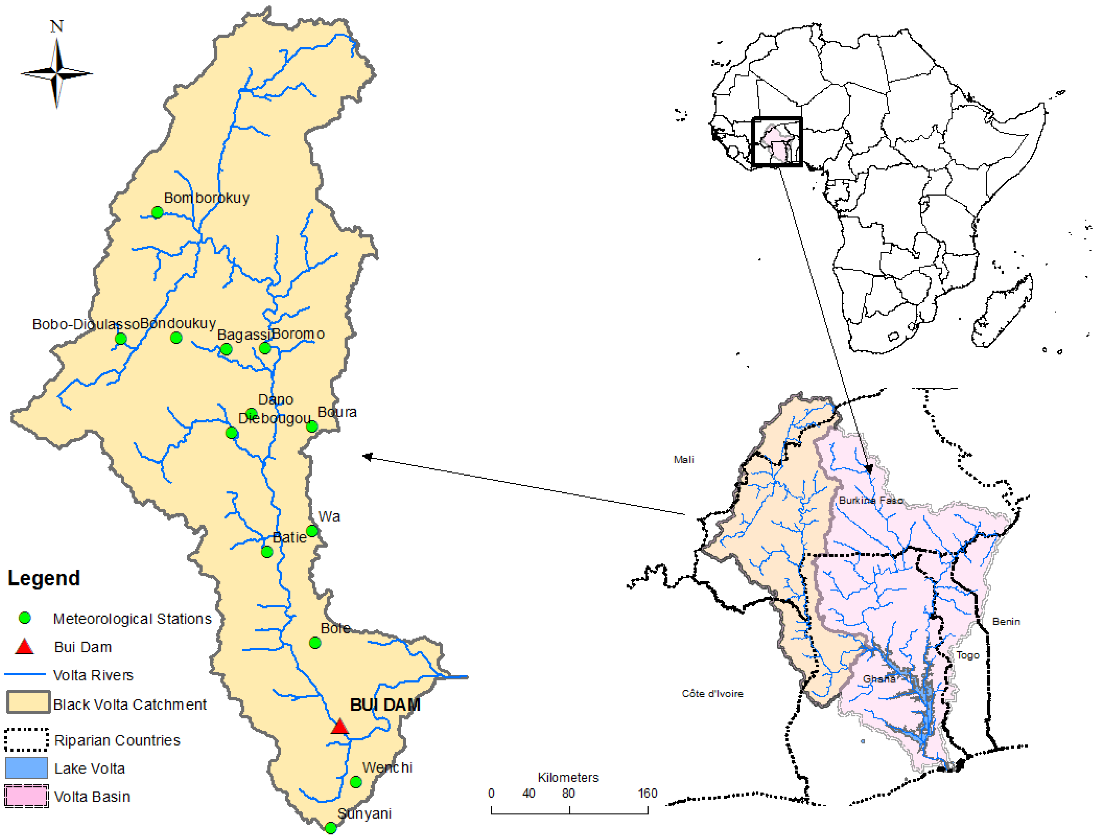
2.1. Study Area Presentation
2.2. Rainfall Data Analysis
2.2.1. Aridity Index
2.2.2. Standardized Precipitation Index
2.2.3. Mann-Kendall Trend Test
2.2.4. Sen’s Slope Estimator
2.3. Land Use and Land Cover Change Maps Development
2.4. Brief Description of the SWAT Model
2.4.1. Surface Runoff
2.4.2. Model Input
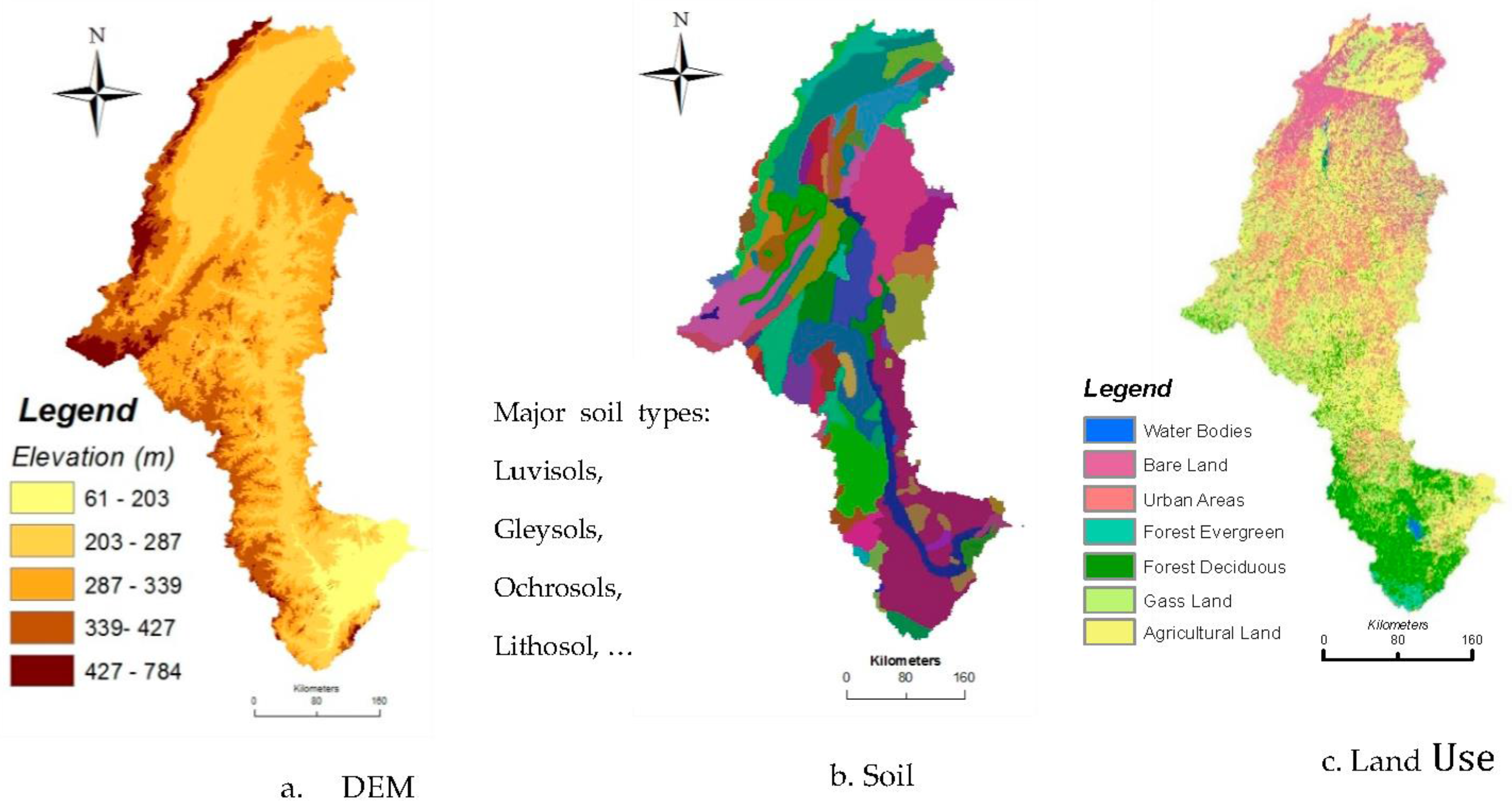
Digital Elevation Model
Soil Data
River Discharge
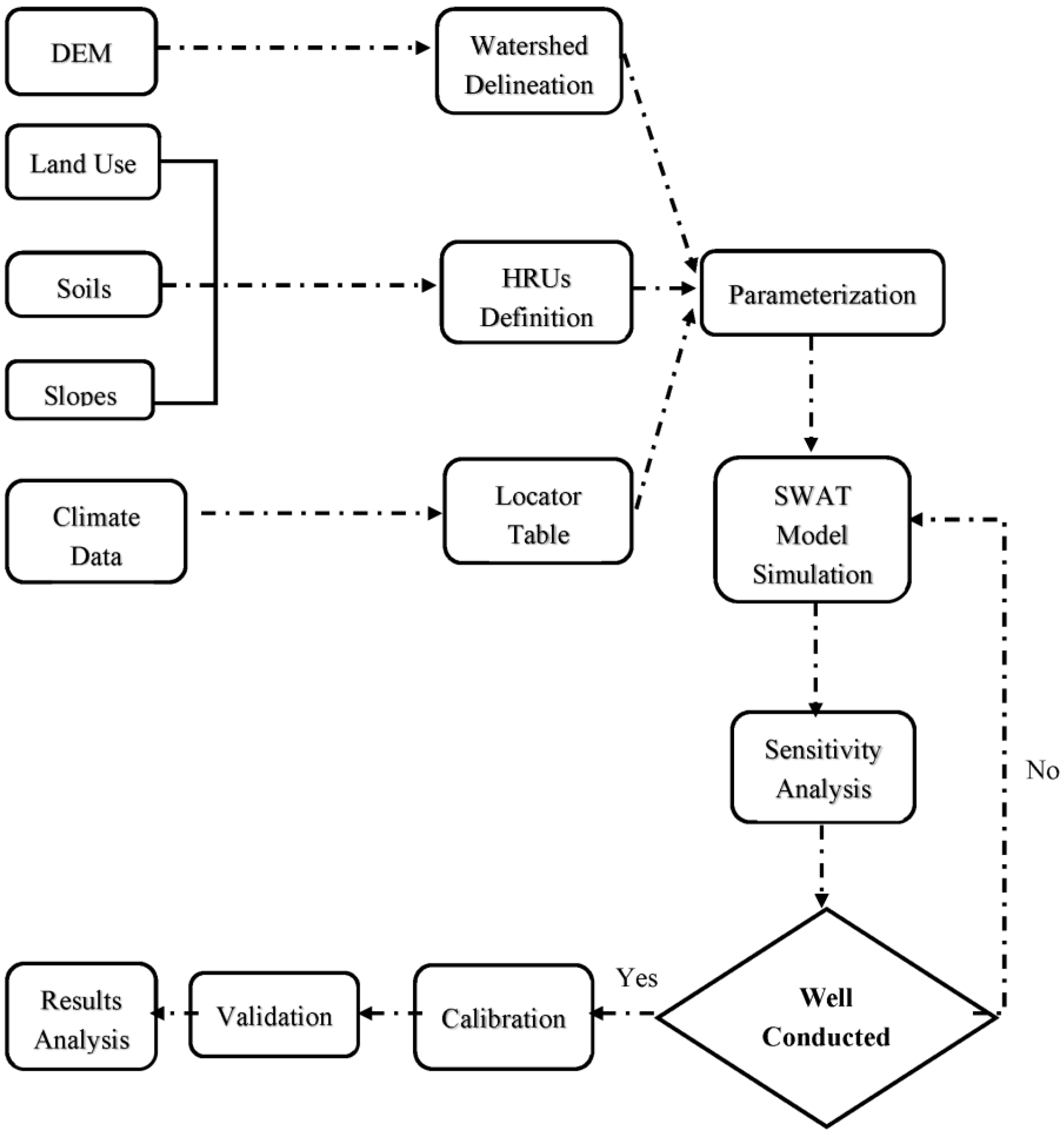
2.4.3. Black Volta Basin Model Set Up
- Goodness of fit or coefficient of determination (R2) between the observation and the final best simulation:
- And the Nash-Sutcliffe (NS) coefficient (Nash et al., 1970) [47]:where: Qobs,i is the observed flow at time i (m3/s), is the mean of observed flow (m3/s), Qsim.i is the simulated flow at time i (m3/s), the mean of simulated flow (m3/s). The Nash-Sutcliffe coefficient rating on monthly time step is given by (Moriasi et al., 2007) [49]. (Awotwi et al., 2015) [14] stated that for model the calibration to be accepted, R2 should be greater than 0.6 and the NS greater than 0.5.
3. Results and Discussions
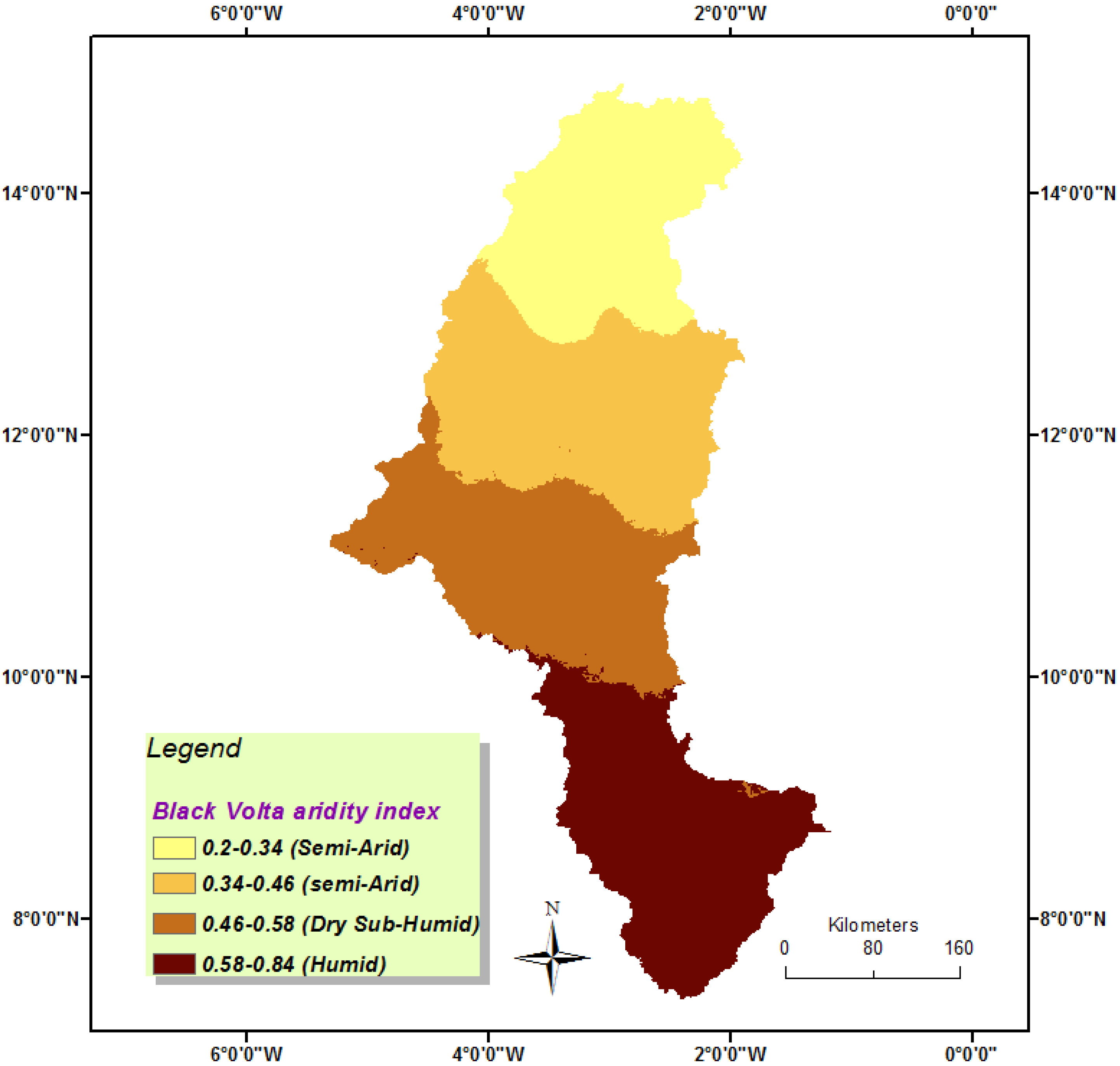
3.1. Aridity Index Profile of the Black Volta and the Standardired Precipitation Index
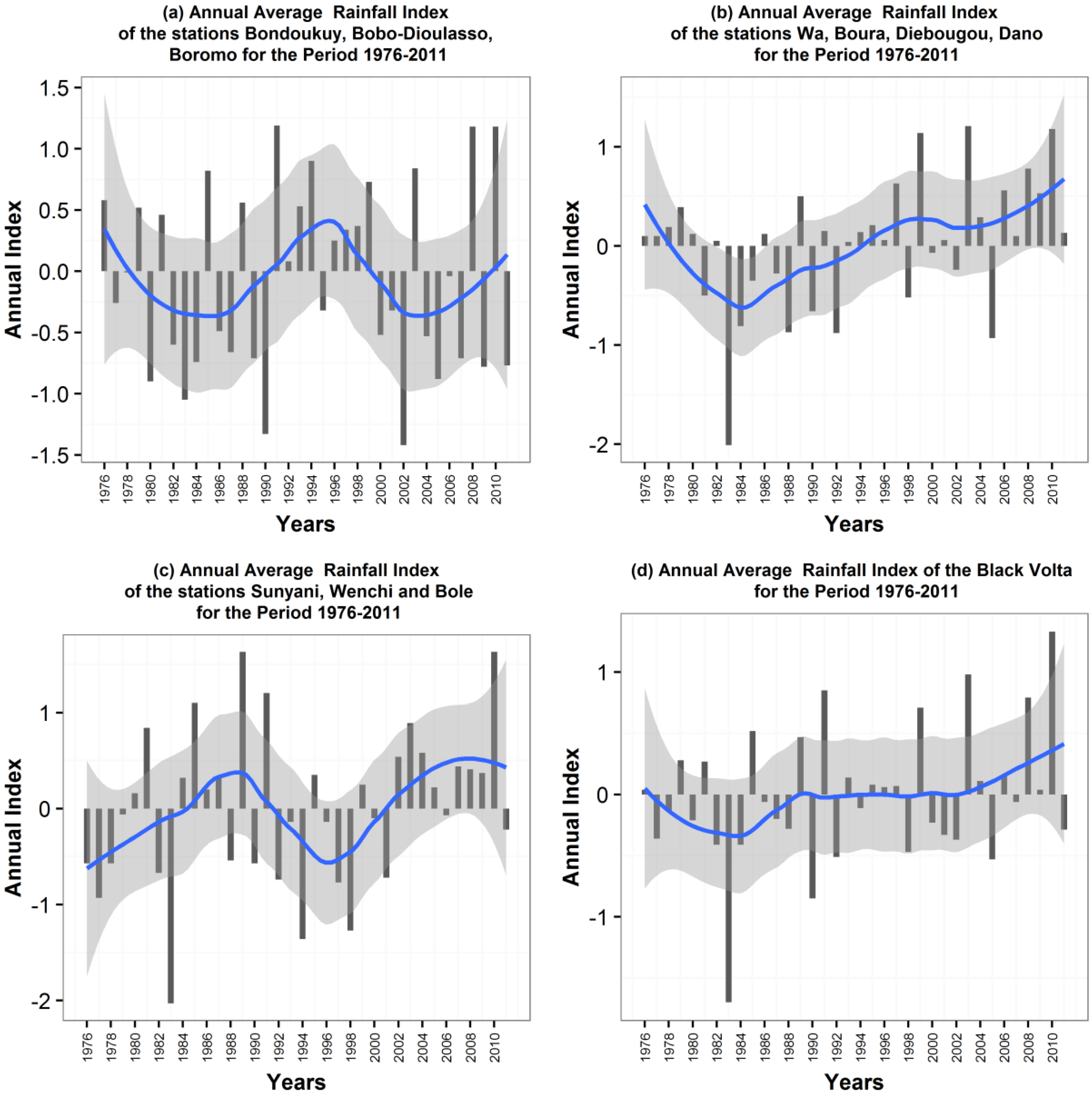
3.2. Rainfall Trend Analysis
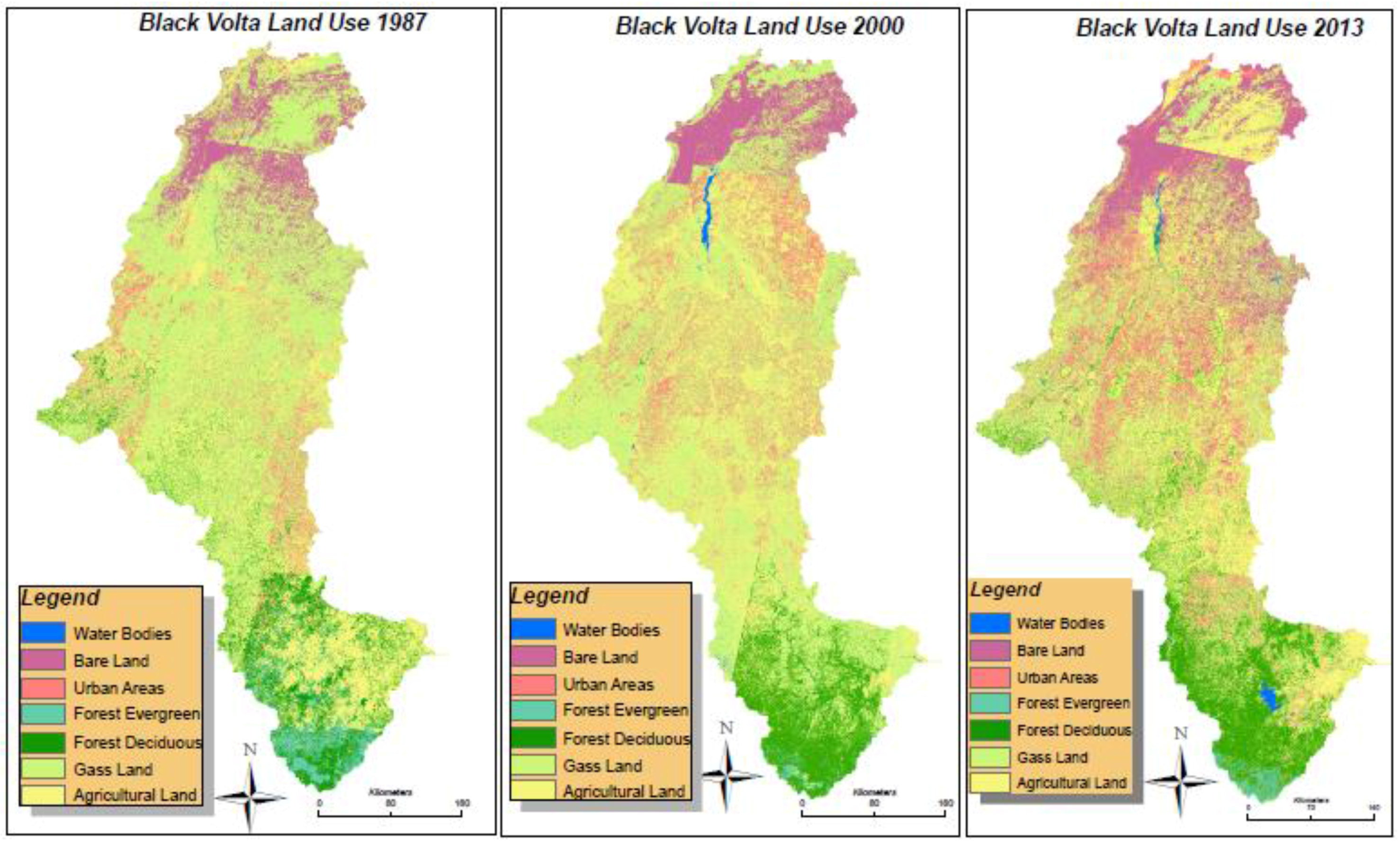
3.3. Land Use and Land Cover Change Analysis
3.4. SWAT Modeling Results
3.4.1. Sensitivity Analysis
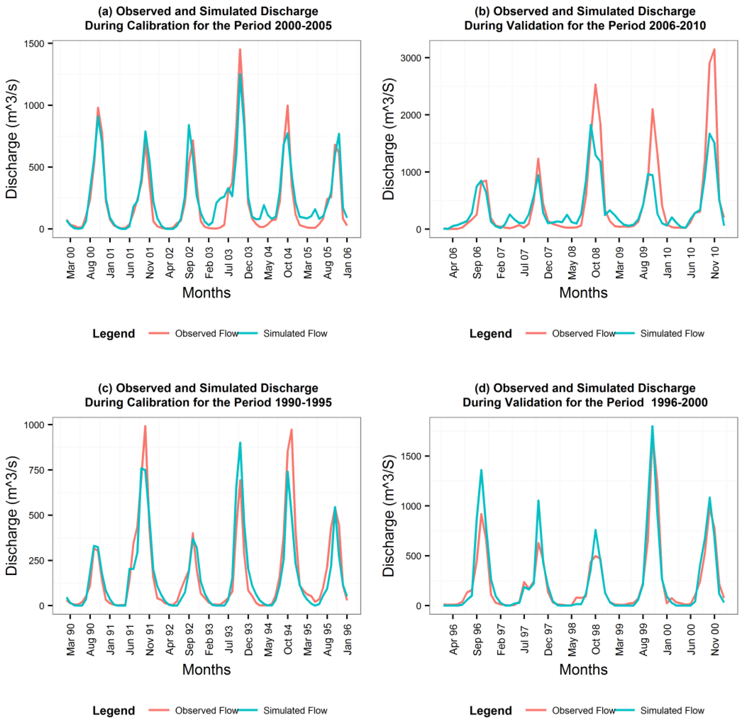
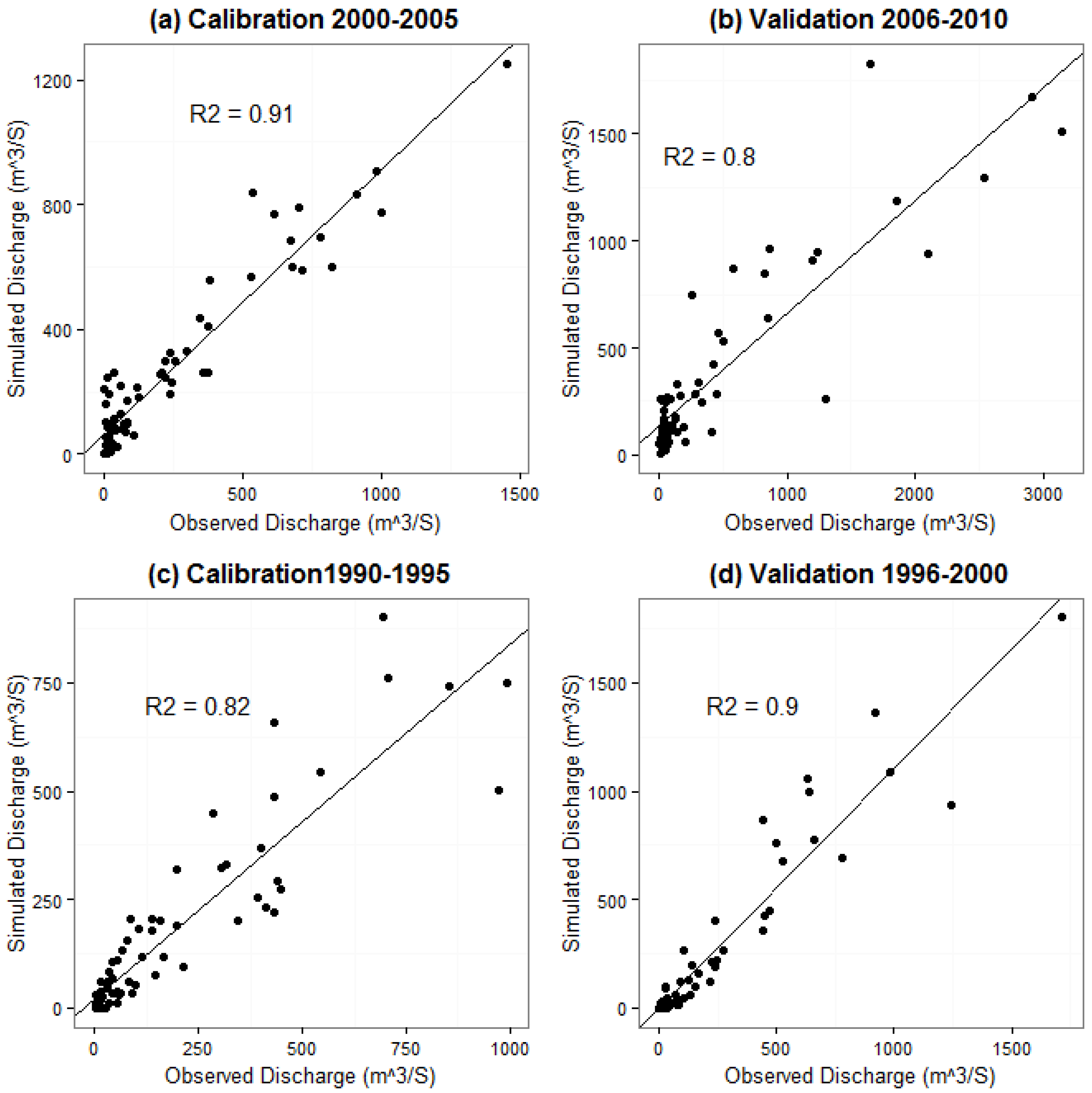
3.4.2. Calibration and Validation
3.4.3. Model Uncertainties
3.4.4. Changes in Seasonal Stream Flow Due to LULC
3.4.5. Changes in Stream Flow Components Due to LULC
4. Conclusions
Acknowledgments
Author Contributions
Conflicts of Interest
Appendix A
Aridity Index
Standardized Precipitation Index
Mann-Kendall Trend Test
Sen’s Slope Estimator
References
- Oguntunde, P.G.; Friesen, J.; van de Giesen, N.; Savenije, H.H.G. Hydroclimatology of the Volta River Basin in West Africa: Trends and variability from 1901 to 2002. Phys. Chem. Earth 2006, 31, 1180–1188. [Google Scholar] [CrossRef]
- Conway, D.; Persechino, A.; Ardoin-Bardin, S.; Hamandawana, H.; Dieulin, C.; Mahé, G. Rainfall and Water Resources Variability in Sub-Saharan Africa during the Twentieth Century. J. Hydrometeorol. 2009, 10, 41–59. [Google Scholar] [CrossRef]
- Mahe, G.; L’Hote, Y.; Olivry, J.C.; Wotling, G. Trends and discontinuities in regional rainfall of West and Central Africa: 1951–1989. Hydrol. Sci. J. 2001, 46, 211–226. [Google Scholar] [CrossRef]
- Owusu, K.; Waylen, P. Trends in spatio-temporal variability in annual rainfall in Ghana (1951–2000). Weather 2009, 64, 115–120. [Google Scholar] [CrossRef]
- Logah, F.Y.; Obuobie, E.; Ofori, D.; Kankam-Yeboah, K. Analysis of Rainfall Variability in Ghana. Int. J. Latest Res. Engineer. Comput. 2013, 1, 1–8. [Google Scholar]
- Lacombe, G.; McCartney, M.; Forkuor, G. Drying climate in Ghana over the period 1960–2005: Evidence from the resampling-based Mann-Kendall test at local and regional levels. Hydrol. Sci. J. 2012, 57, 1594–1609. [Google Scholar] [CrossRef]
- Andreini, M.; van de Giesen, N.; van Edig, A.; Fosu, M.; Andah, W. Volta Basin Water Balance; ZEF: Bonn, Germany, 2000. [Google Scholar]
- Arnold, J.G.; Kiniry, J.R.; Srinivasan, R.; Williams, J.R.; Haney, E.B.; Neitsch, S.L. Soil and Water Assessment Tool, Input/output File Documentation; Technical Report 439; Texas Water Research Institute: College Station, TX, USA, 2012. [Google Scholar]
- Neitsch, S.L.; Arnold, J.G.; Kiniry, J.R.; Srinivasan, R.; Williams, J.R. Soil and Water Assessment Tool Input/Output File Documentation; Blackland Research Center: Temple, TX, USA, 2005. [Google Scholar]
- Setegn, S.G.; Srinivasan, R.; Dargahi, B. Hydrological modelling in the Lake Tana Basin, Ethiopia using SWAT model. Open Hydrol. J. 2008, 2, 49–62. [Google Scholar] [CrossRef]
- Malunjkar, V.S.; Shinde, M.G.; Ghotekar, S.S.; Atre, A.A. Estimation of Surface Runoff using SWAT Model. Int. J. Latest Res. Engineer. Comput. 2015, 3, 12–15. [Google Scholar]
- Easton, Z.M.; Fuka, D.R.; White, E.D.; Collick, A.S.; Ashagre, A.B.; McCartney, M.; Awulachew, S.B.; Ahmed, A.A.; Teenhuis, T.S. A multi basin SWAT model analysis of runoff and sedimentation in the Blue Nile, Ethiopia. Hydrol. Earth System Sci. 2010, 14, 1827–1841. [Google Scholar] [CrossRef]
- Spruill, C.A.; Workman, S.R.; Taraba, J.L. Simulation of Daily and Monthly Stream Discharge from Small Watershed Using the SWAT Model. Am. Soc. Agric. Eng. 2000, 1, 1431–1439. [Google Scholar] [CrossRef]
- Awotwi, A.; Kumi, M.; Pe, J.; Yeboah, F.; Nti, I.K. Predicting Hydrological Response to Climate Change in the White Volta. J. Earth Sci. Clim. Chang. 2015, 6, 1–7. [Google Scholar] [CrossRef]
- Obuobie, E. Estimation of Groundwater Recharge in the Context of Future Climate Change in the White Volta River Basin, West Africa; ZEF: Bonn, Germany, 2008. [Google Scholar]
- Schuol, J.; Abbaspour, K.C. Calibration and uncertainty issues of a hydrological model (SWAT) applied to West Africa. Adv Geosci. 2006, 2, 137–143. [Google Scholar] [CrossRef]
- Allwaters Consult. Diagnostic Study of The Black Volta Basin in Ghana; Final Report; ALLWATERS Consult Limited: Kumasi, Ghana, June 2012. [Google Scholar]
- Green Cross International, Burkina Faso, 2001. Trans-boundary Basin Sub-Projects: The Volta River Basin. Available online: www.greencrossitalia.it/ita/acqua/wfp/pdf/greencrosswfp_volta.pdf (accessed on 15 January 2016).
- Barry, B.; Obuobie, E.; Andreini, M.; Andah, W.; Pluquet, M. The Volta River Basin: Comparative Study of River Basin Development and Management. Comprehensive Assessment of Water Management in Agriculture; IWMI: Colombo, Sri Lanka, 2005. [Google Scholar]
- Shaibu, S.; Odai, S.N.; Adjei, K.A.; Osei, E.M.; Annor, F.O. Simulation of runoff for the Black Volta Basin using satellite observation data. Int. J. River Basin Manag. 2012, 10, 245–254. [Google Scholar] [CrossRef]
- Peterson, T.C.; Easterling, D.R.; Karl, T.R.; Groisman, P.; Nicholls, N.; Plummer, N.; Vincent, L. Homogeneity adjustments of in situ atmospheric climate data: A review. Int. J. Climatol. 1998, 18, 1493–1517. [Google Scholar] [CrossRef]
- Reeves, J.; Chen, J.; Wang, X.L.; Lund, R.; Lu, Q.Q. A review and comparison of changepoint detection techniques for climate data. J. Appl. Meteorol. Climatol. 2007, 46, 900–915. [Google Scholar] [CrossRef]
- Searcy, J.K.; Hardison, C.H. Double-Mass Curves; US Government Printing Office: Washington, WA, USA, 1960.
- Westmacott, J.R.; Burn, D.H. Climate change effects on the hydrologic regime within the Churchill-Nelson River Basin. J. Hydrol. 1997, 202, 263–279. [Google Scholar] [CrossRef]
- Cannarozzo, M.; Noto, L.V.; Viola, F. Spatial distribution of rainfall trends in Sicily (1921–2000). Phys. Chem. Earth 2006, 31, 1201–1211. [Google Scholar] [CrossRef]
- Liu, Q.; Yang, Z.; Cui, B. Spatial and temporal variability of annual precipitation during 1961–2006 in Yellow River Basin, China. J. Hydrol. 2008, 361, 330–338. [Google Scholar] [CrossRef]
- Zhang, Y.; Guan, D.; Jin, C.; Wang, A.; Wu, J.; Yuan, F. Analysis of impacts of climate variability and human activity on streamflow for a river basin in northeast China. J. Hydrol. 2011, 410, 239–247. [Google Scholar] [CrossRef]
- Gocic, M.; Trajkovic, S. Analysis of changes in meteorological variables using Mann-Kendall and Sens slope estimator statistical tests in Serbia. Glob. Planet. Chang. 2013, 100, 172–182. [Google Scholar] [CrossRef]
- Lanzante, J.R. Resistant, Robust and Non-Parametric Techniques for the Analysis of Climate Data: Theory and Examples, Including Applications to Historical Radiosonde Station Data. Int. J. Climatol. 1996, 16, 1197–1226. [Google Scholar] [CrossRef]
- Kendall, M.G. Rank Correlation Methods; Hafner Press: New York, NY, USA, 1962. [Google Scholar]
- Ahmad, I.; Tang, D.; Wang, T.; Wang, M.; Wagan, B. Precipitation Trends over Time Using Mann-Kendall and Spearman’s Rho Tests in Swat River Basin, Pakistan. Adv. Meteorol. 2015, Article ID 431860. [Google Scholar] [CrossRef]
- Hirsch, R.M.; Alexander, R.B.; Smith, R.A. Selection of methods for the detection and estimation of trends in water quality. Water Resour. Rese. 1991, 27, 803–813. [Google Scholar] [CrossRef]
- Tabari, H.; Marofi, S.; Aeini, A.; Talaee, P.H.; Mohammadi, K. Trend analysis of reference evapotranspiration in the western half of Iran. Agric. For. Meteorol. 2011, 151, 128–136. [Google Scholar] [CrossRef]
- Bayazit, M.; Önöz, B.; Yue, S.; Wang, C. Comment on “Applicability of prewhitening to eliminate the influence of serial correlation on the Mann-Kendall test” by Sheng Yue and Chun Yuan Wang. Water Resour. Res. 2004, 40, 1–5. [Google Scholar] [CrossRef]
- Sen, P.K. Estimates of the Regression Coefficient Based on Kendall’s Tau. J. Am. Stat. Assoc. 1968, 63, 1379–1389. [Google Scholar] [CrossRef]
- Van Vliet, J.; Bregt, A.K.; Hagen-Zanker, A. Revisiting Kappa to account for change in the accuracy assessment of land-use change models. Ecol Modell. 2011, 222, 1367–1375. [Google Scholar] [CrossRef]
- Stehman, S.V.; Czaplewski, R.L. Design and Analysis for Thematic Map Accuracy Assessment—An application of satellite imagery. Remote Sens. Environ. 1998, 64, 331–344. [Google Scholar] [CrossRef]
- Foody, G.M. Status of land cover classification accuracy assessment. Remote Sens. Environ. 2002, 80, 185–201. [Google Scholar] [CrossRef]
- Zăvoianu, F.; Caramizoiub, A.; Badeaa, D. Study and Accuracy Assessment of Remote Sensing Data for Environmental Change Detection in Romanian Coastal Zone of the Black Sea. In Proceedings International Society for Photogrammetry and Remote Sensing, Istanbul, Turkey, 12–23 July 2004.
- Carletta, J. Assessing agreement on classification tasks: The kappa statistic. Comput. Linguist. 1996, 22, 249–254. [Google Scholar]
- Neitsch, S.L.; Williams, J.R.; Arnold, J.G.; Kiniry, J.R. Soil and Water Assessment Tool Theoretical Documentation; Version 2009; Texas Water Resources Institute: College Station, TX, USA, 2011. [Google Scholar]
- United States. Soil Conservation Service. Hydrology. In SCS National Engineering Handbook; U.S Department of Agriculture: Washington, WA, USA, 1972; Section 4. [Google Scholar]
- Green, W.H.; Ampt, G.A. Studies on Soil Phyics. J. Agric. Sci. 1911, 4, 1. [Google Scholar] [CrossRef]
- NRCS. In Urban Hydrology for Small Watersheds TR-55; U.S Department of Agriculture: Washington, WA, USA, 1986.
- Abbaspour, K.C.; Vejdani, M.; Haghighat, S.; Yang, J. SWAT-CUP Calibration and Uncertainty Programs for SWAT. Fourth Int. SWAT Conf. 2007, 1596–1602. [Google Scholar]
- Abbaspour, K.C.; Johnson, C.A.; van Genuchten, M.T. Estimating Uncertain Flow and Transport Parameters Using a Sequential Uncertainty Fitting Procedure. Vadose Zone J. 2004, 3, 1340–1352. [Google Scholar] [CrossRef]
- Nash, J.E.; Sutcliffe, J.V. River flow forecasting through conceptual models part I—A discussion of principles. J. Hydrol. 1970, 10, 282–290. [Google Scholar] [CrossRef]
- Abbaspour, K.C. SWAT-CUP 2012: SWAT calibration and uncertainty Programs-A user manual; Eawag (Swiss Federal Institute of Aquatic Science and Technology): Zurich, Switzerland, 2013. Available online: swat.tamu.edu/media/114860/usermanual_swatcup.pdf (accessed on 29 June 2016).
- Moriasi, D.; Arnold, J. Model evaluation guidelines for systematic quantification of accuracy in watershed simulations. Trans. ASABE 2007, 50, 885–900. [Google Scholar] [CrossRef]
- L’Hôte, Y.; Mahé, G.; Somé, B.; Triboulet, J.P. Analysis of a Sahelian annual rainfall index from 1896 to 2000; the drought continues. Hydrol. Sci. J. 2002, 47, 563–572. [Google Scholar] [CrossRef]
- Anderson, J.R. A land use and land cover classification system for use with remote sensor data. US Government Printing Office: Washington, WA, USA, 1976. [Google Scholar]
- Adjei, K.A.; Ren, L.; Appiah-adjei, E.K.; Odai, S.N. Application of satellite-derived rainfall for hydrological modelling in the data-scarce Black Volta trans-boundary basin. Hydrol. Res. 2015, 46, 777–791. [Google Scholar] [CrossRef]
- Zomer, R.J.; Trabucco, A.; Bossio, D.A.; Verchot, L.V. Climate change mitigation: A spatial analysis of global land suitability for clean development mechanism afforestation and reforestation. Agric. Ecosyst. Environ. 2008, 126, 67–80. [Google Scholar] [CrossRef]
- Allen, R.G.; Pereira, L.S.; Raes, D.; Smith, M. Crop Evapotranspiration-Guidelines for Computing Crop Water Requirements-FAO Irrigation and Drainage Paper 56; FAO: Rome, Italy, 1998. [Google Scholar]
- Mcleod, A.A.I. Kendall rank correlation and Mann-Kendall trend test. Available online: https://cran.r-project.org/web/packages/Kendall/ (accessed on 25 June 2016).
- Hollander, M.; Wolfe, D.A.; Chicken, E. Nonparametric Statistical Methods; John Wiley & Sons: Hoboken, NJ, USA, 2013. [Google Scholar]
- Jassby, A.D.; Cloern, J.E. wq: Exploring water quality monitoring data. Available online: https://www.icesi.edu.co/CRAN/web/packages/wq/ (accessed on 25 June 2016).


| Country | Gauging Station | Lat (°N) | Lon (°W) | Elevation (m) |
|---|---|---|---|---|
| Ghana | Sunyani | 7.3328 | −2.3281 | 296 |
| Ghana | Wenchi | 7.75 | −2.1 | 322 |
| Ghana | Bui | 8.2361 | −2.2772 | 176 |
| Ghana | Bole | 9.0319 | −2.4762 | 295 |
| Ghana | Wa | 10.0667 | −2.5 | 262 |
| Burkina Faso | Batie | 9.8739 | −2.9213 | 298 |
| Burkina Faso | Diebougou | 10.9667 | −3.25 | 298 |
| Burkina Faso | Boura | 11.0333 | −2.5 | 306 |
| Burkina Faso | Dano | 11.1490 | −3.2931 | 304 |
| Burkina Faso | Boromo | 11.75 | −2.9333 | 260 |
| Burkina Faso | Bondoukuy | 11.8450 | −3.7639 | 326 |
| Burkina Faso | Bobo-Dioulasso | 11.1605 | −4.3298 | 374 |
| Burkina Faso | Bomborokuy | 12.9972 | −3.9496 | 344 |
| Gauging Station | Tau | p-Value | Zs | Qs med or Sen’s Slope Estimator | Constant B |
|---|---|---|---|---|---|
| Sunyani | 0.156 | 0.1864 | 1.321 | 0.3437 | 93.12 |
| Wenchi | 0.073 | 0.5399 | 0.6129 | 0.1197 | 101.68 |
| Bui | −0.0724 | 0.4535 | −0.7497 | −0.1283 | 94.11 |
| Bole | 0.18 | 0.1271 | 1.55 | 0.3961 | 82.17 |
| Wa | 0.127 | 0.2819 | 1.076 | 0.1749 | 83.29 |
| Batie | −0.0635 | 0.5953 | −0.531 | −0.1559 | 88.69 |
| Diebougou | 0.106 | 0.3686 | 0.899 | 0.1178 | 83.47 |
| Boura | 0.279 | 0.0171 | 2.38 | 0.3218 | 70.02 |
| Dano | 0.143 | 0.2254 | 1.21 | 0.222 | 72.03 |
| Boromo | 0.113 | 0.3403 | 0.954 | 0.1754 | 68.17 |
| Bondoukuy | −0.132 | 0.6728 | −0.422 | −0.0936 | 71.85 |
| Bobo-Dioulasso | −0.0635 | 0.5952 | −0.5312 | −0.1683 | 84.75 |
| Bomborokuy | −0.126 | 0.2584 | −1.13 | −0.2106 | 62.73 |
| Year | Overall Accuracy | Kappa Coefficient |
|---|---|---|
| 1987 | 90.20 | 88.57 |
| 2000 | 93.06 | 91.90 |
| 2013 | 99.18 | 99.05 |
| Land Cover Type | Area Coverage (km2) | Area Coverage (%) | 1987–2000 | 2000–2013 | 1987–2013 | |||||||
|---|---|---|---|---|---|---|---|---|---|---|---|---|
| 1987 | 2000 | 2013 | 1987 | 2000 | 2013 | Change (%) | Change Rate (%/year) | Change (%) | Change Rate (%/year) | Change (%) | Change Rate (%/year) | |
| Bare Land | 13231.9 | 11279.37 | 18842.86 | 8.5 | 7.3 | 12.15 | −14.76 | −1.05 | 67.06 | 4.79 | 42.4 | 1.57 |
| Urban Areas | 9619.8 | 16537.32 | 22030.4 | 6.2 | 10.7 | 14.21 | 71.91 | 5.14 | 33.22 | 2.37 | 129.01 | 4.78 |
| Water Bodies | 101.7 | 872.6904 | 939.15 | 0.1 | 0.6 | 0.61 | 758.1 | 54.15 | 7.62 | 0.54 | 823.45 | 30.5 |
| Agricultural Land | 36125.7 | 36796.48 | 47710.4 | 23.3 | 23.7 | 30.77 | 1.86 | 0.13 | 29.66 | 2.12 | 32.07 | 1.19 |
| Grass Land | 76253.9 | 74198.44 | 41151.4 | 49.2 | 47.9 | 26.54 | −2.7 | −0.19 | −44.54 | −3.18 | −46.03 | −1.7 |
| Forest Deciduous | 14034.6 | 14398.31 | 23063.6 | 9.1 | 9.3 | 14.87 | 2.57 | 0.19 | 60.18 | 4.3 | 64.33 | 2.38 |
| Forest Evergreen | 5708.9 | 967.4019 | 1338.64 | 3.7 | 0.6 | 0.86 | −83.05 | −5.93 | 38.38 | 2.74 | −76.55 | −2.84 |
| Parameter Name | Definition | Absolute SWAT Values | Fitted Value | Minimum Value | Maximum Value | Sensitivity Rank |
|---|---|---|---|---|---|---|
| R__SOL_K | Saturated hydraulic conductivity | 0–2000 | −0.999737 | −1.009404 | −0.966056 | 1 |
| V__MSK_CO2 | Calibration coefficient used to control impact of the storage time constant for low flow | 0–10 | 3.117479 | 2.870465 | 5.470611 | 2 |
| V__SURLAG | Surface runoff lag time | 0.05–24 | 22.728235 | 22.493849 | 22.75284 | 3 |
| V__MSK_CO1 | Calibration coefficient used to control impact of the storage time constant for normal flow | 0–10 | 10.726233 | 9.479877 | 14.147874 | 4 |
| R__SOL_AWC | Available water capacity of the soil layer | 0–1 | 0.201121 | 0.145896 | 0.2093 | 5 |
| R__CN2 | SCS runoff curve number f | −0.2–0.2 | −0.537993 | −0.552411 | −0.505139 | 6 |
| A__GWQMN | Threshold depth of water in the shallow aquifer required for return flow to occur (mm) | 0–5000 | 73.4655 | 73.35611 | 74.378479 | 7 |
| V__ALPHA_BF | Base flow alpha factor (days) | 0–1 | −0.155831 | −0.160484 | −0.153358 | 8 |
| V__GW DELAY | Groundwater delay (days) | 0–500 | 1.087874 | 0.994085 | 1.122037 | 9 |
| V__RCHRG_DP | Deep aquifer percolation fraction | 0–1 | 0.159342 | 0.148055 | 0.176487 | 10 |
| V__ESCO | Soil evaporation compensation factor | 0–1 | 0.599675 | 0.595305 | 0.646715 | 11 |
| V__CH_N2 | Manning’s “n” value for the main channel | −0.01–0.3 | 0.267461 | 0.242134 | 0.271966 | 12 |
| Period | Average Monthly Flow (m3/s) | Standard Deviation (m3/s) | Model Performance | |||||
|---|---|---|---|---|---|---|---|---|
| Measured | Simulated | Measured | Simulated | P-Factor | R-Factor | R2 | NS | |
| Calibration (2000–2005) | 223.16 | 252.70 | 306.38 | 274.3 | 0.64 | 0.66 | 0.91 | 0.9 |
| Validation (2006–2010) | 447.99 | 371.23 | 730.94 | 433.84 | 0.2 | 0.33 | 0.80 | 0.7 |
| Period | Average Monthly Flow (m3/s) | Standard Deviation (m3/s) | Model Performance | |||||
|---|---|---|---|---|---|---|---|---|
| Measured | Simulated | Measured | Simulated | P-Factor | R-Factor | R2 | NS | |
| Calibration (1990–1995) | 172.28 | 161.79 | 234.95 | 212.24 | 0.97 | 0.83 | 0.82 | 0.9 |
| Validation (1996–2000) | 229.18 | 254.37 | 338.39 | 394.68 | 0.64 | 0.9 | 0.85 | 0.7 |
| LULC 2000 | LULC 2013 | Mean Monthly Flow Change | |||
|---|---|---|---|---|---|
| Dry Months (Jan, Feb, Mar) | Wet Months (Aug, Sep, Oct) | Dry Months (Jan, Feb, Mar) | Wet Months (Aug, Sep, Oct) | Dry | Wet |
| 238.62 | 2969.02 | 253.42 | 2995.35 | +6% | +1% |
| Stream Flow Components (m3/s) and ET (mm) | LULC 2000 | LULC 2013 | Changes (%) |
|---|---|---|---|
| SURF_Q | 376.7 | 477.3 | 27% |
| LAT_Q | 5.7 | 6.8 | 19% |
| GW_Q | 828 | 775.1 | −6% |
| WATER_YIELD | 1210.4 | 1259.2 | 4% |
| ET | 521.6 | 546.7 | 4.59% |
© 2016 by the authors; licensee MDPI, Basel, Switzerland. This article is an open access article distributed under the terms and conditions of the Creative Commons Attribution (CC-BY) license (http://creativecommons.org/licenses/by/4.0/).
Share and Cite
Akpoti, K.; Antwi, E.O.; Kabo-bah, A.T. Impacts of Rainfall Variability, Land Use and Land Cover Change on Stream Flow of the Black Volta Basin, West Africa. Hydrology 2016, 3, 26. https://doi.org/10.3390/hydrology3030026
Akpoti K, Antwi EO, Kabo-bah AT. Impacts of Rainfall Variability, Land Use and Land Cover Change on Stream Flow of the Black Volta Basin, West Africa. Hydrology. 2016; 3(3):26. https://doi.org/10.3390/hydrology3030026
Chicago/Turabian StyleAkpoti, Komlavi, Eric Ofosu Antwi, and Amos T. Kabo-bah. 2016. "Impacts of Rainfall Variability, Land Use and Land Cover Change on Stream Flow of the Black Volta Basin, West Africa" Hydrology 3, no. 3: 26. https://doi.org/10.3390/hydrology3030026