Modeling watershed runoff and erosion processes realistically requires field determination or model calibration estimation of surface soil infiltration rates or effective hydraulic conductivities (Km) and erosion rates because they vary with soil cover/tilth/slope conditions, and seasonally with changing water contents. The field methods often used to measure in situ saturated or effective hydraulic conductivities (Ks or Km, respectively, where Km is some fraction of Ks) include surface (e.g., disk, single/double-ring infiltrometers, and rainfall simulators), or subsurface techniques (e.g., bore-hole methods). Indirect estimates of Km and erodibilities available from NRCS soil survey information that are typically derived from soil texture information are also more often used in modeling than field measured values due to the difficulty associated with the field measurements and their variability. While each measurement method may have particular advantages depending on the intended use of the data, surface methods enable measurement of actual conditions as affected by soil tilth and surface cover while also providing insights into the effectiveness of soil restoration methods in the field. However, they are not without complications associated with surface disturbance/roughness, type and configuration of surface cover, steep slope (double-ring methods require mild slopes), disk plate hydraulic contact and estimation from rainfall minus runoff rates using rainfall simulators. Similarly, subsurface measurement techniques or Km estimation from soil texture information may miss the effect of surface layers on infiltration storage or excess leading to runoff–erosion prediction failure.
1.1. Brief Literature Review
Rainfall simulators (RSs) are essential tools for investigating the dynamic processes of infiltration, runoff and erosion under a variety of field conditions [
1,
2,
3,
4], and information from RS test plots can provide the infiltration/runoff parameterization required for watershed modeling. Though multiple RS designs for field application exist, no single RS design (including plot runoff frame installation) has emerged as a standard. Similarly, while in RS plot tests, typically, data about rainfall, runoff and erosion rates and time to runoff are collected from which infiltration rates, or K
m and erodibilities are estimated, no standard RS data analysis methodology has evolved. Despite a number of years of research into the plant/cover effects on soil erosion [
5,
6,
7,
8,
9,
10,
11,
12], it remains difficult to understand erosion processes and mechanics due to the lack of sufficiently comparable data or results [
8,
13]. Moreover, the differences in soil properties, slope surface conditions and vegetation types in field experiments have tended to complicate interpretations of field measurements. It is difficult, therefore, to draw meaningful comparisons between RS plot data reported in different studies [
2,
3,
4,
14,
15]. In addition, there are few, if any, actual comparisons of RS performance with respect to infiltration, erosion, or soil detachment rates. For example, Lascelles et al. [
16] only considered the variability in drop sizes, distributions and energies from two different RSs and speculated on implications with respect to erosion, but did not offer comparison RS plot studies. Similarly, Kinnell [
17,
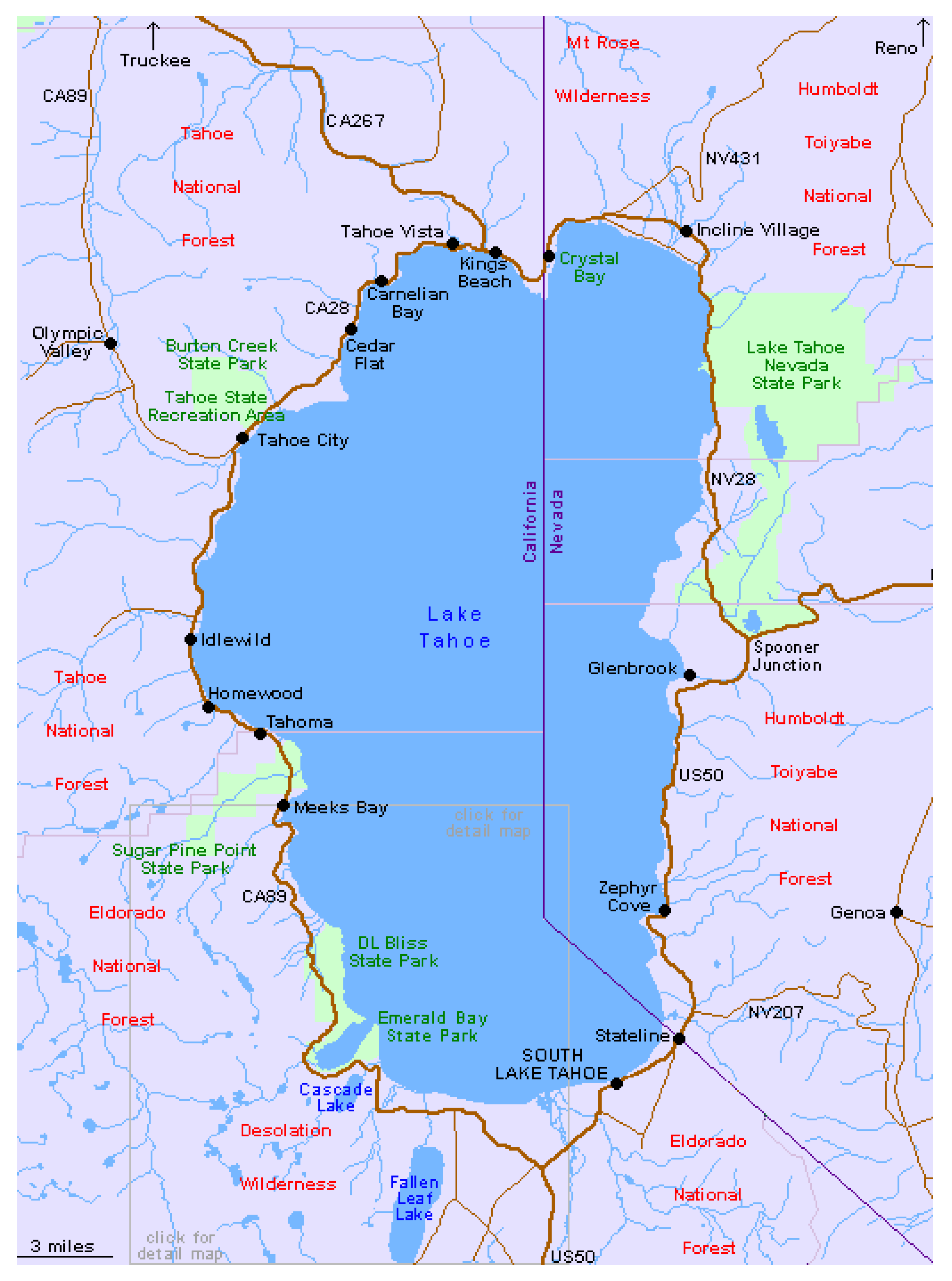
18] completed thorough reviews of the processes associated with raindrop impacted erosion and noted that both conceptual models and measurements fail in various respects to adequately characterize field observed erosion processes from bare soils. Concerns such as these have also arisen in the Tahoe Basin, because a variety of methods for measurement of infiltration and erosion rates have been deployed, but comparisons between results of different studies remain less than definitive.
1.3. Theory—Infiltration Equation Development
Several infiltration equations have been derived during the past few decades and the most often used in watershed modeling revolve around time-to-ponding estimates and the ponded infiltration Green–Ampt type square-wave wetting-front formulation, among others. In RS plot studies, the applied rainfall rates are generally large and for durations that exceed that of natural rainfall so as to achieve runoff after some acceptable elapsed time after rainfall initiation. As such, there are typically a few minutes during which the plot infiltration capacity exceeds that of the applied rainfall followed by shallow ponded infiltration. Ideally, the effective hydraulic conductivity that satisfies both the time-to-ponding and ponded infiltration equations would represent the self-consistent field value that then should apply in watershed modeling. We briefly define terms and develop these equations here, eventually coupling the ponding time and Green–Ampt–type equations to allow implicit determination of Km from the RS data outlined above.
Basic definitions from Grismer [
19] include:
where h
d = displacement pressure head (mm), and h
c = capillary pressure head (mm)
where S = saturation, S
r = residual saturation, S
m= maximum saturation associated with infiltration, and λ = pore-size distribution index.
And the Green–Ampt infiltration equation takes the form
where I = infiltration rate (mm/hr),
Km = “natural saturated hydraulic conductivity” (mm/hr) ≈ 0.5Ks,
H= ponding depth (mm),
hf = wetting front capillary pressure head (mm), and
zf = wetting front depth (mm).
Combining the Green–Ampt Equation (3) with the continuity equation yields
where V = volume infiltrated per unit area (mm).
The Green–Ampt equation above is readily modified to account for air resistance to wetting flow by using β to replace the 1 at the beginning of the RHS of Equation (4) and h
f within the parentheses with H
c [
19]. β and H
c are defined as follows
where μ
w and μ
g are the water and air viscosities, respectively, similalry k
rw and k
rg are the relative permeabilities of the porous media to water and air, respectively. S
e is the effective saturation and
fw is the fractional flow function of water, or the ratio of water flow to total (air and water) flowrate. For all practical purposes, β takes on a value between 1.2 and 1.3 for typical λ values between 2 and 3, an index range that covers loamy to sandy soils [
19]. The wetting front driving head, H
c can be determined from
where h
e is defined in Equation (1). Again for all practical purposes, H
c takes on a value between 1.12 h
d – 1.08 h
d for λ between 2 and 3. Substituting Equations (5) and (6) in the Green–Ampt Equation (4) to correct for air resistance or counterflow during infiltration results in [
19]
Finally, the corresponding ‘time–to-ponding’ infiltration equation that accounts for air resistance or counterflow as well is given by
where q
o is the rainfall rate and
fw is practically zero for ponded infiltration (see Morel-Seytoux [
20] discussion linking the transition of rainfall rate controlled infiltration conditions to that for ponded infiltration).
With a relationship between h
d and K
m together with the time-to-ponding, infiltrated depth and times from RS plot data, Equations (7) and (8) can be solved simultaneously for K
m (assuming that K
m = 0.5 K
s) by solving Equation (8) for φ(S
m − S
i) and letting
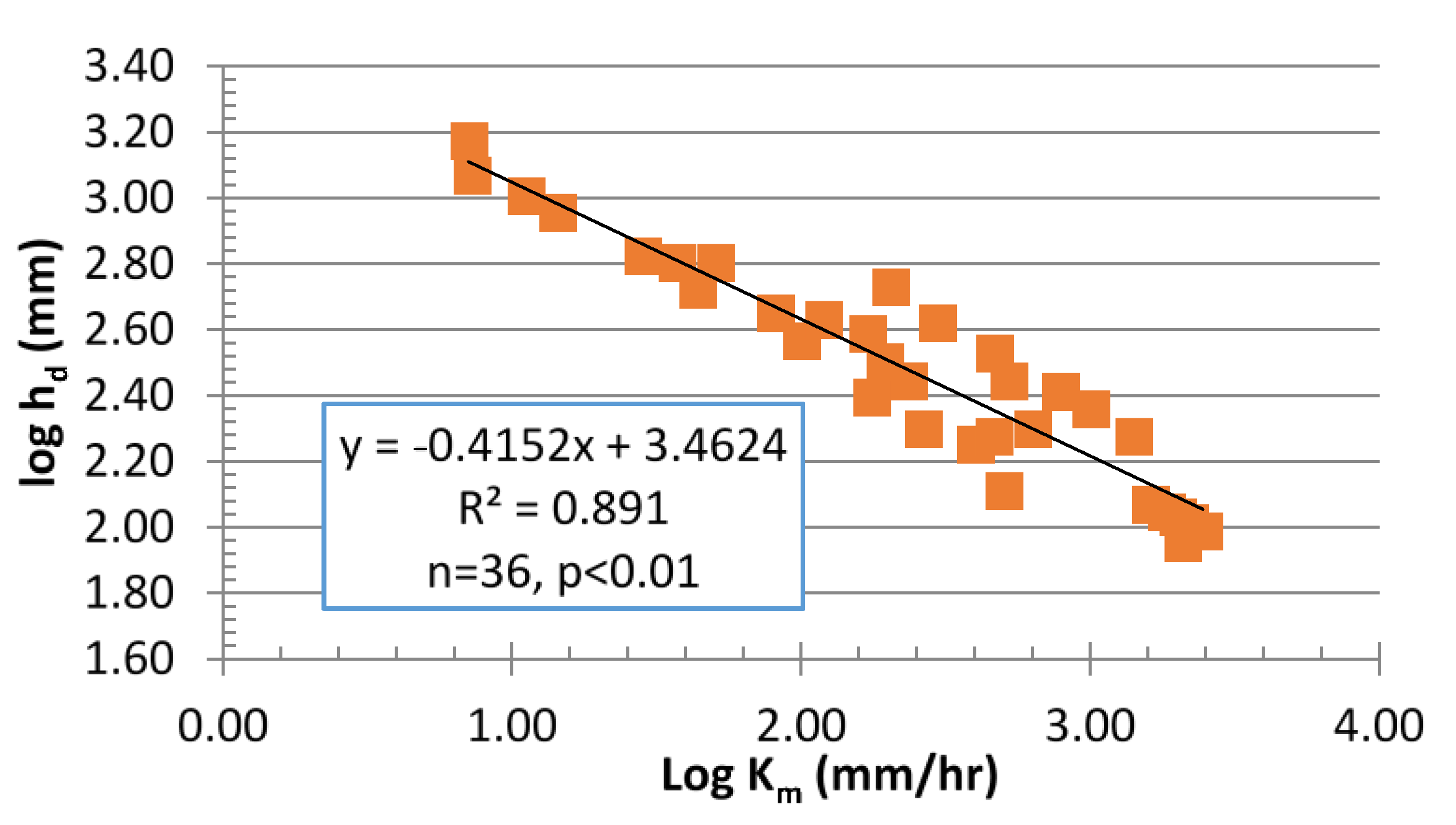
fwi = 0. Using lab column data collected to date, Grismer [
19] determined that for h
d in meters, the semi-empirical theoretical relationship for permeability was k (μm
2) ≈ 0.84/h
d2. Using only that lab data for sands that more closely replicate the Tahoe soils and changing to more directly applicable units, we found that K
m (mm/hr) = 19.9/h
d2.4 for h
d (mm), as shown in
Figure 1. And as noted above, taking H
c 1.1 h
d, β
1.3 for λ = 3, and the ponded depth H of Equations (4) or (7) as typically assumed to be small (e.g., 1 mm as in watershed modeling, [
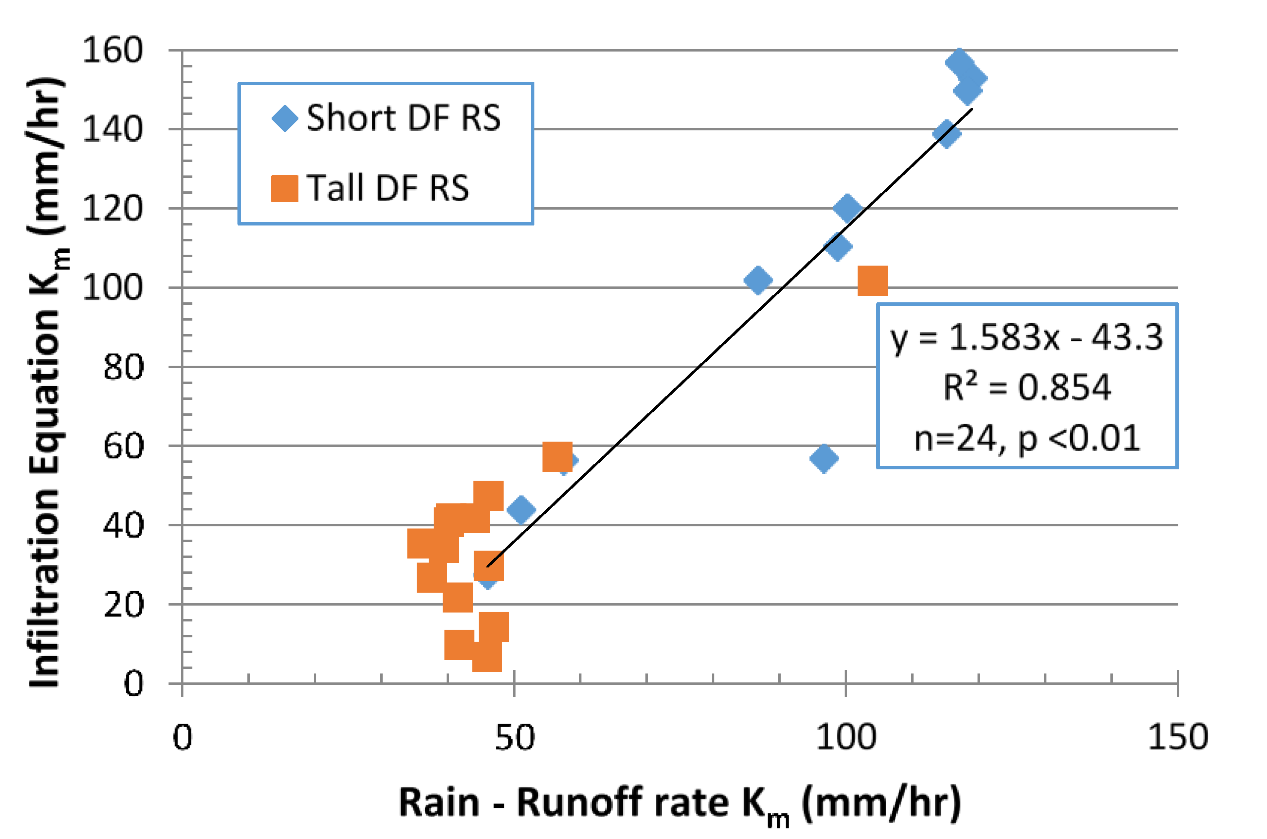
21]), we can implicitly solve for K
m from Equations (7) and (8) by re-arranging Equation (8) to solve for ∆θ = φ(S
m − S
i), as shown below as Equation (9) and substituted into Equation (7).
Alternatively, we can use the simpler Main–Larson equations analogous to Equations (7) and (9) below, but still accounting for air-resistance to infiltration
and
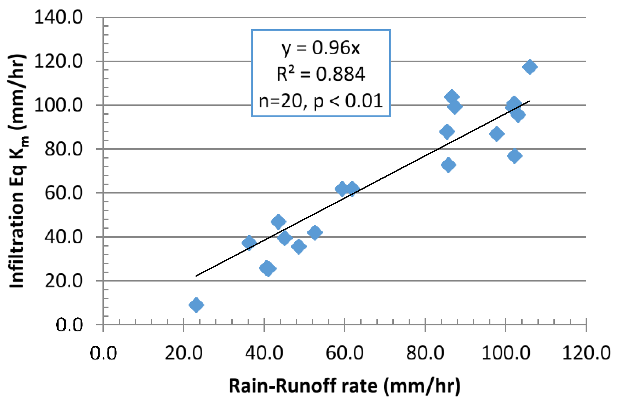
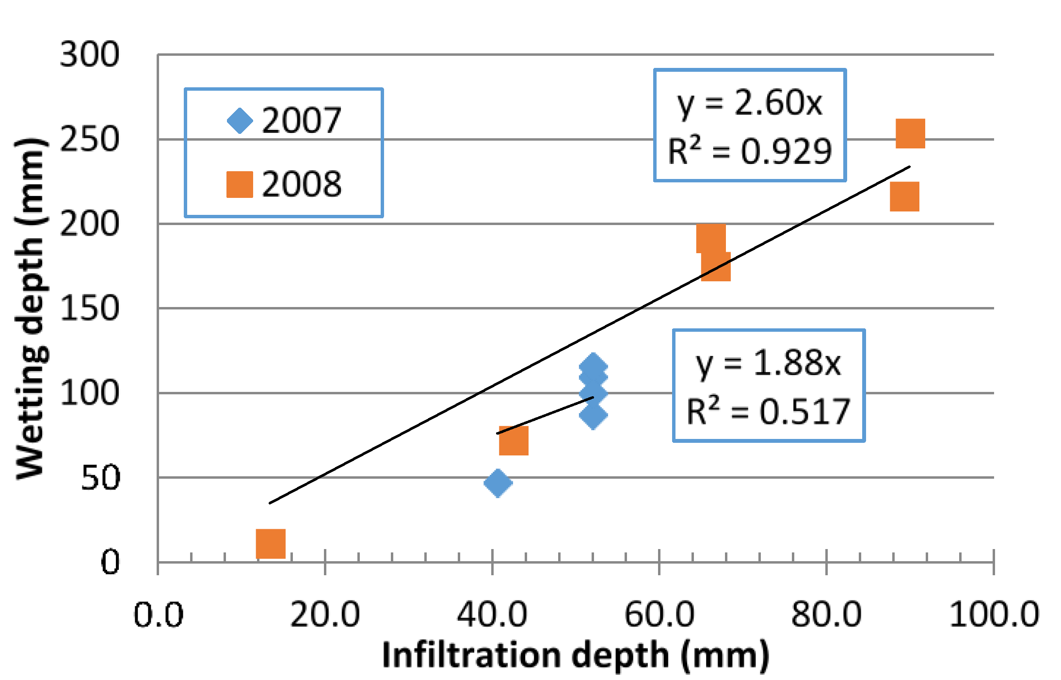
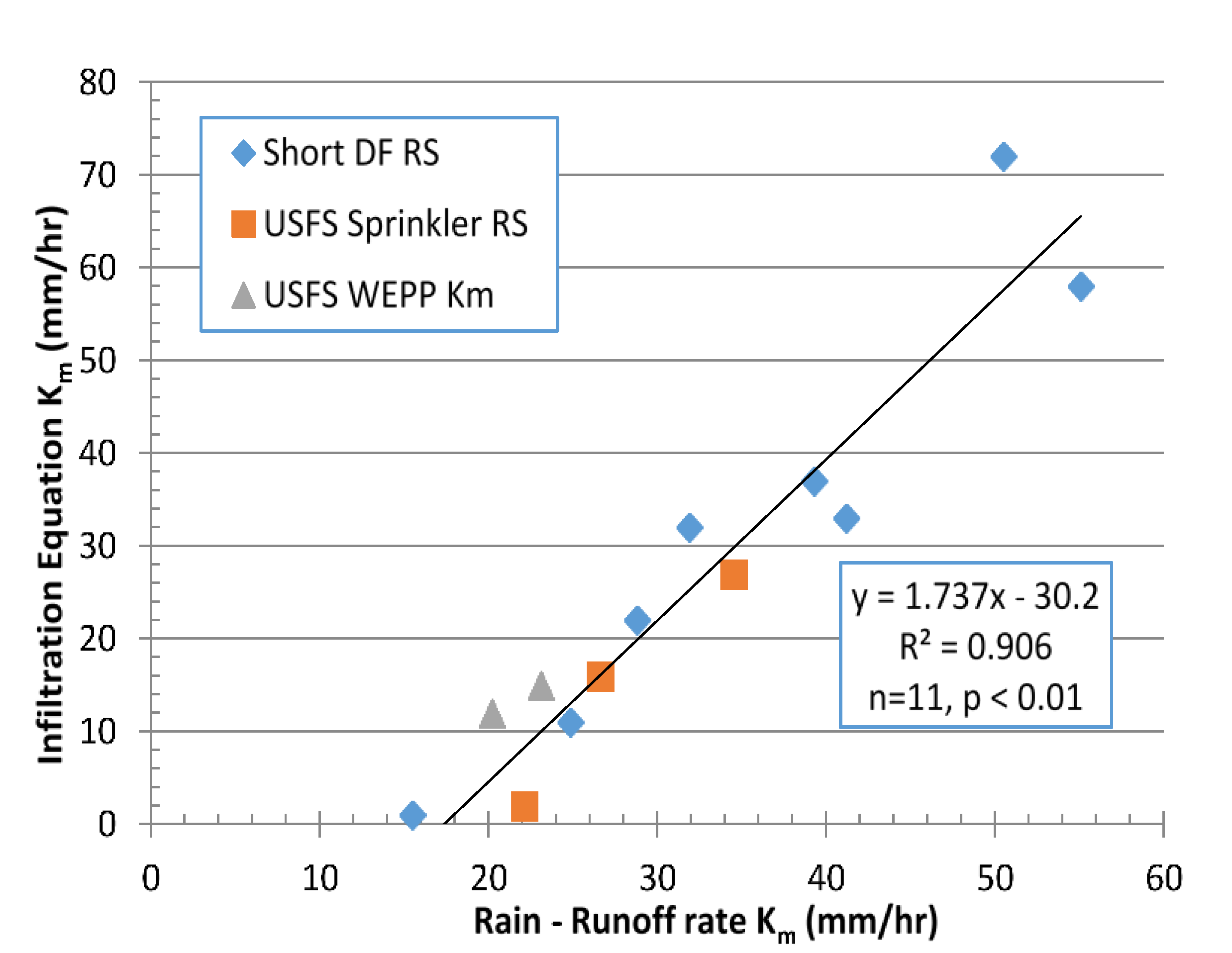
Finally, we can use the estimated effective ∆θ, taken as the measured infiltrated depth compared to the visual wetting front depth, from RS plot data when no runoff occurs, combined with the infiltrated depth and RS test duration to determine K
m from Equation (7). For example,
Figure 2 shows the relationship between visual wetting and infiltrated depths from the long-term monitoring site at Heavenly ski area on the coarser-textured granitic soils where the average regression slope suggests an effective ∆θ
45%.
1.4. Theory—Erosion Equation Development
Most watershed modeling efforts and associated estimation of sediment detachment or erosion rates employ the well-known Manning’s equation to relate overland or channel flowrates and velocity to flow depth and hillslope, or channel gradient. Of course, use of Manning’s equation implies that an appropriate surface roughness value, “n”, can be identified, that the driving force, or slope angle <10% and that flows are fully turbulent. The assumption of turbulent flow conditions during sheet flow across the RS plot or the landscape is questionable when flow depths are quite small and laminar flows are more likely present [
21]. The general derivation of the laminar flow equation for thin films on inclined planes at any angle, α, to the horizontal requires only the assumptions of the “no-slip” boundary condition together with constant fluid properties [
22]. Considering two-dimensional steady laminar flow of depth, y, down an inclined plane at angle, α, to the horizontal, the shear force as given by the fluid viscosity, μ, and the parabolic velocity function is balanced by the gravitational force (unit weight, ρg) on the fluid body in the direction of flow. That is, the flowrate Q per unit width is given by
where u
m is the mean velocity taken as 2/3
rds of the maximum velocity assuming a parabolic velocity distribution perpendicular to the inclined plane. Of course, the equivalent flowrate equation assuming turbulent flow and mild slopes (<10%) is taken from the approximation for the Chezy–Mannings equation assuming flow depths are very small compared to flow width, B,
The flow mean velocity needed to determine shear stresses on soil particles is given by Q/y from Equations (12) or (13), depending on whether laminar or turbulent flow is assumed. Replacing the sine function with a power function approximation in Equation (14), it is apparent that under steady laminar flow conditions the mean surface flow velocity is practically proportional to the slope, S, rather than the square root of the slope, as in the mean velocity determined from Manning’s Equation (15); moreover, there is no slope limitation or need to identify the roughness value, “n”.
In RS plot studies, the runoff rate, q, is often expressed as the steady flowrate collected at the runoff lip frame divided by the area of the plot, as this allows convenient comparison to the infiltration and rainfall rates, and because rarely is the actual sheet flow depth measured or estimated so as to enable calculation of the mean, or average, overland flow velocity, u
m. The relationship between q and u
m is simply given by the mass balance
where A = runoff frame area (m
2), B = the runoff lip width (m) and the other parameters are as previously defined. Solving Equation (16) for the mean velocity then requires substitution for the flow depth based on either Equation (15) for turbulent flow, or Equation (14) for laminar flow, as shown below, respectively, in Equations (17) and (18).
Quantitative description of soil particle detachment or erosion processes perhaps originated with Ellison’s [
23] observation that “erosion is a process of detachment and transport of soil materials by erosive agents”. These “erosive agents”, of course, include raindrop impact and overland flow. Of course, rain drop impact energy diminishes with increasing flow depth and presence of soil cover that both “absorb” the drop impact energy. Raindrop impact energy, while an erosive agent on bare soils should probably be related to the aggregate strength, that is, the energy needed to break up and mobilize surface aggregates [
24,
25]. Subsequent research, more or less, begins with Ellison’s paradigm of sorts that continues in concept through the soil-detachment equation review by Owoputi and Stolte [
26]. Similarly, Foster and Meyer [
27] interpreted results of several experiments in terms of Yalin’s equation that assumes “sediment motion begins when the lift force of flow exceeds a critical force … necessary to … carry the particle downstream until the particle weight forces it out the flow and back to the bed.” Bridge and Dominic [
28] built on this concept and described the critical velocities and shears needed for single particle transport over fixed rough planar beds. Gilley et al. [
29,
30,
31] included the Darcy–Weisbach friction factor as a measure of the resistance to flow that was eventually adopted in the WEPP model. Moore and Birch [
32] combined slope and velocity and suggested that particle transport and transport capacity for both sheet (interrill) and rill flows is best derived from the unit stream power. In all these descriptions, the erodibility process essentially involves momentum transfer with an energy loss to friction. More recently, the concept of stream power as the primary factor controlling soil detachment rates has been adopted in several reviews e.g., [
33,
34,
35,
36]. Assuming turbulent and laminar flow conditions, respectively, from Equations (17) and (18), stream power,
P, can be expressed as
and
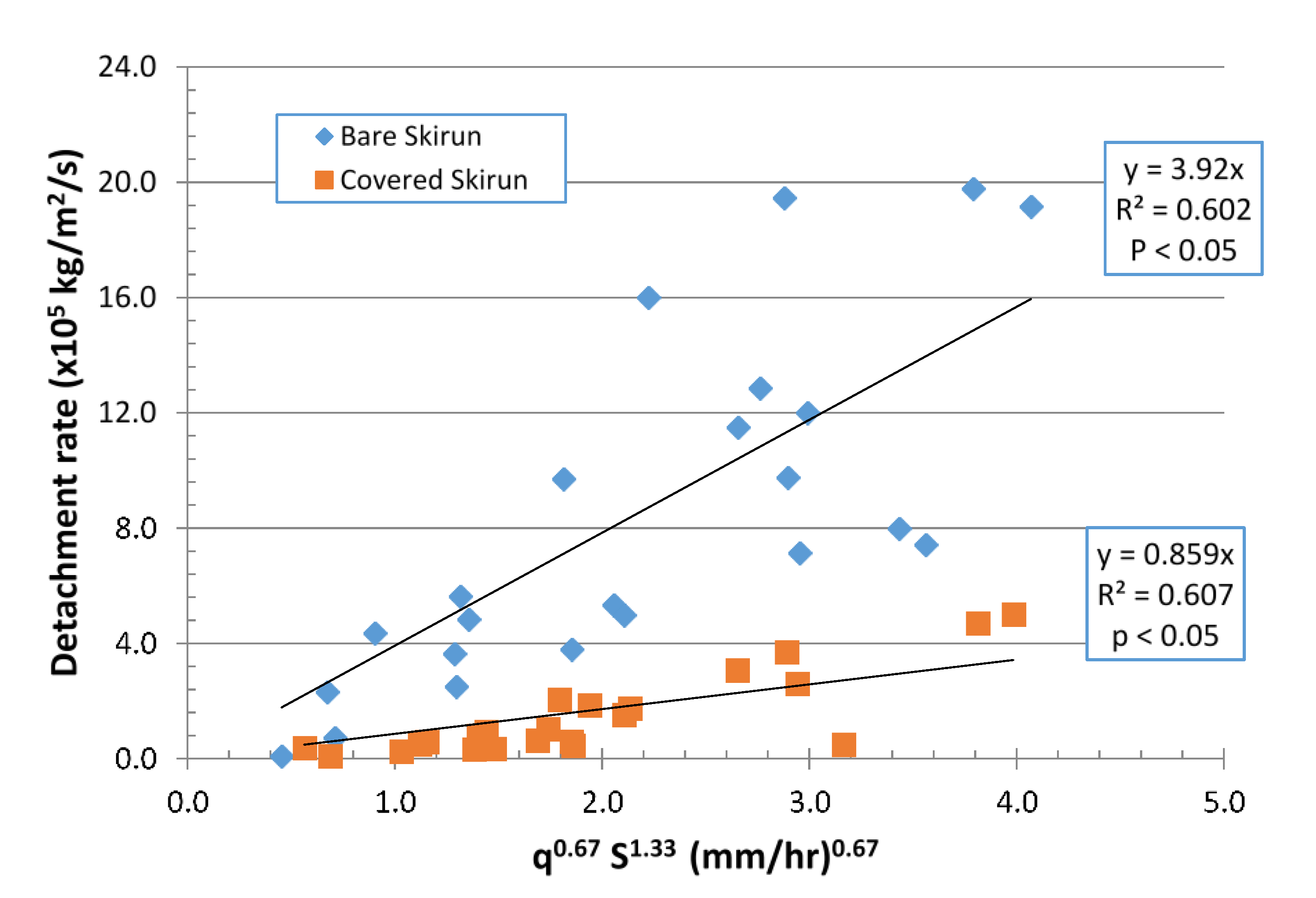
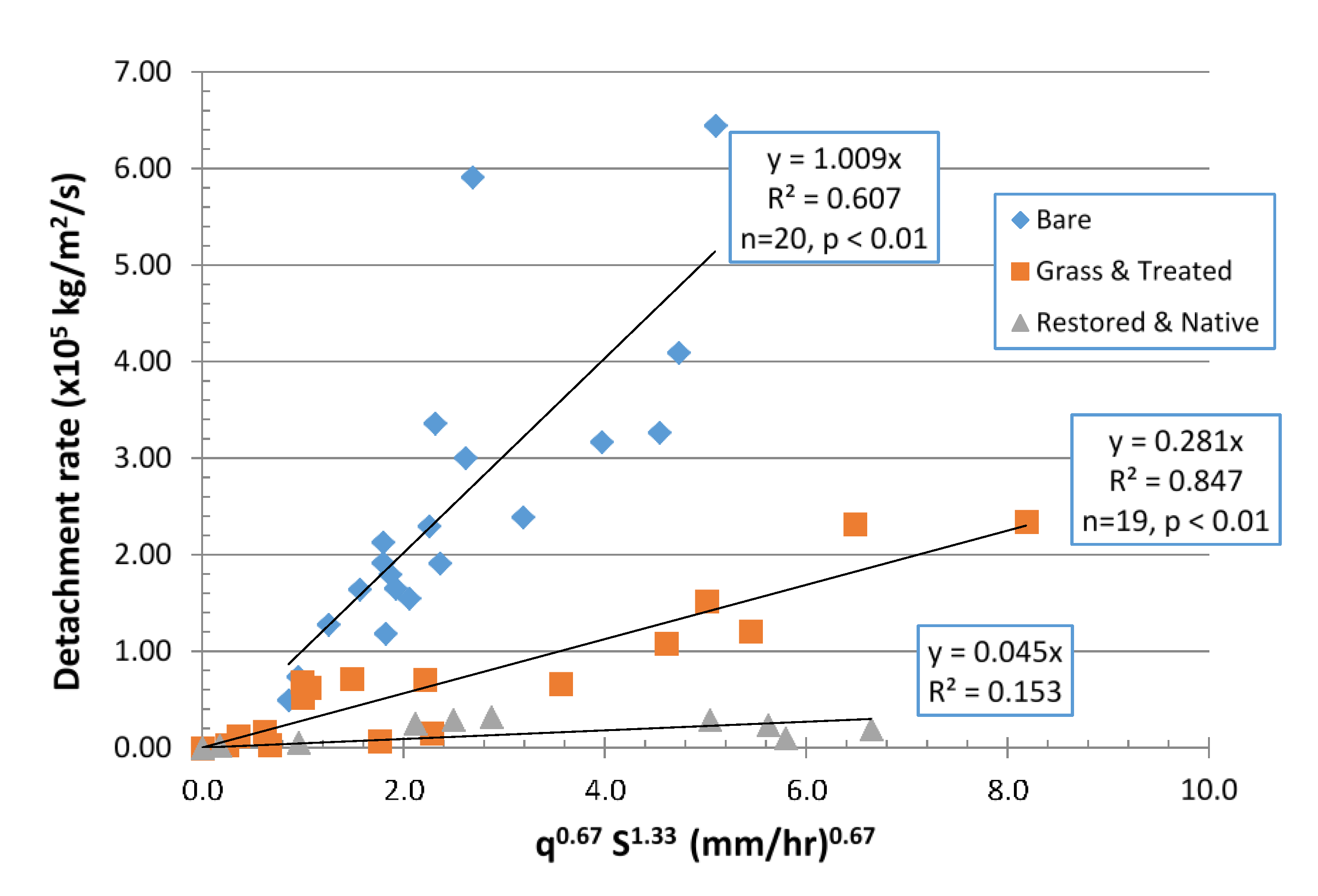
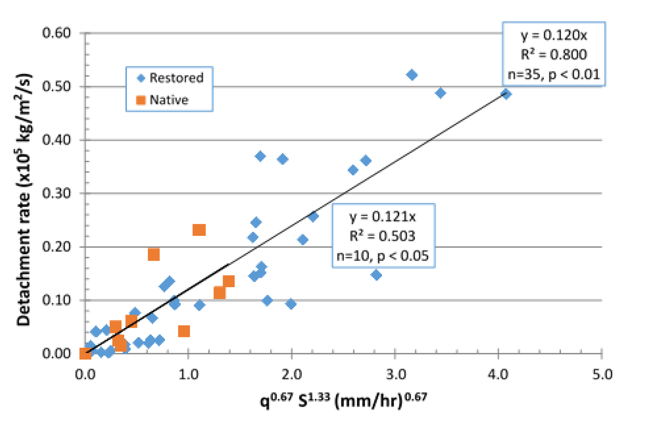
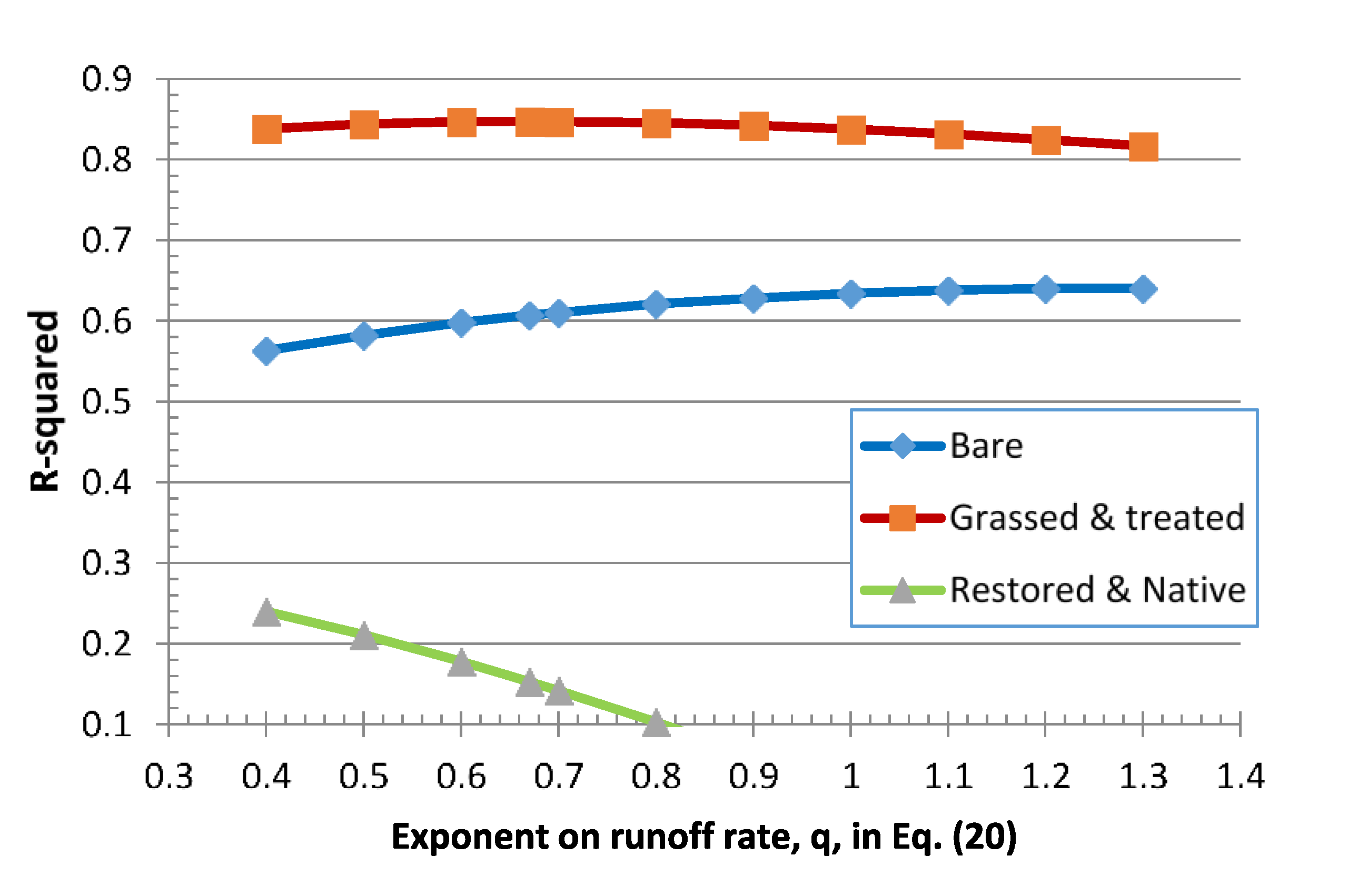
Note that in both Equations (19) and (20), slope, S, has a practically the same effect on stream power, hence detachment rate, whether the flow is laminar or turbulent; that is, P is proportional to S~1.3. However, the runoff rate under laminar flow conditions has a much greater affect than that under turbulent flow conditions (i.e., P is proportional to q0.67 as compared to q0.4), as do the unit weight and plot dimensions (though offset to some degree by ‘n’). Nonetheless, in terms of practical analyses of RS plot runoff and erosion data, when rain splash impacts are negligible, it is apparent that the soil particle detachment rate is proportional to ~S1.3 and , where ‘a’ takes on a value between 0.4 and 0.7.
Experimentally, the dependence of stream power on slope between laminar and turbulent flow is not well articulated. In fact, at slopes of 4%–12%, McCool et al. [
37] found soil loss rates dependent on S
1.37–S
1.5, rather than S~
1.3. In flume studies, Zhang et al. [
38] found across a slope range of 3%–47% their detachment data was proportional to q
2.04 S
1.27 suggesting that both Equations (19) and (20) may underestimate the effects of runoff rate. At small slopes, detachment rate was more sensitive to q than S, however, as S increased, its influence on detachment rate increased. Later, Zhang et al. [
39] found that for undisturbed “natural” soils across a similar slope range (9%–47%), detachment rates were most proportional to q
0.89 S
1.02. In contrast, on nearly flat slopes (1%–2%) with deep flow depths (~10 mm), Nearing and Parker [
40] found that turbulent flow resulted in far greater soil detachment rates than did laminar flow, in part as a result of greater shear stresses. Following Gilley and Finkner [
29], Guy et al. [
41] examined the effects of raindrop impact on interrill sediment transport capacity in flume studies at 9%–20% slopes. Assuming a laminar flow regime, they found that raindrop splash accounted for ~85% of the transport capacity, in some contrast to earlier studies indicating that raindrop impact had little or no effect on slopes greater than about 10%. Sharma et al. [
42,
43,
44] systematically examined rain splash effects on aggregate breakdown and particle transport in the laboratory but did not relate their results to stream power. At larger slopes, Lei et al. [
45] found that both slope and runoff rate were important towards transport capacity on slopes up to about 44%, but that transport capacity increased only slightly at still steeper slopes. Zhang et al. [
39] found the best linear regression quantifying soil detachment rates occurred for equations that included the square of the rainfall rate (I
2) times the WEPP slope factor, or I times the runoff rate and slope, S, as compared to I times the square root of the runoff rate times S
0.67. This observation of a better fit with the first two equations suggested that detachment rate is proportional to stream power. Similarly, considering soil detachment from overland flow only across a range of burned, disturbed and relatively undisturbed rangeland soils with slopes of 6%–57%, Al-Hamdan et al. [
35] found that detachment rates were proportional to
P1.18, but that the exponent of 1.18 did not differ significantly from unity. Gabriels [
34] found that detachment rates were related to
P1.3 for a range of clay fractions of 7%–41%, an exponent value consistent with that for the plot slope in Equations (19) and (20). In the RS plot studies considered here, we assume that detachment rates are proportional to S
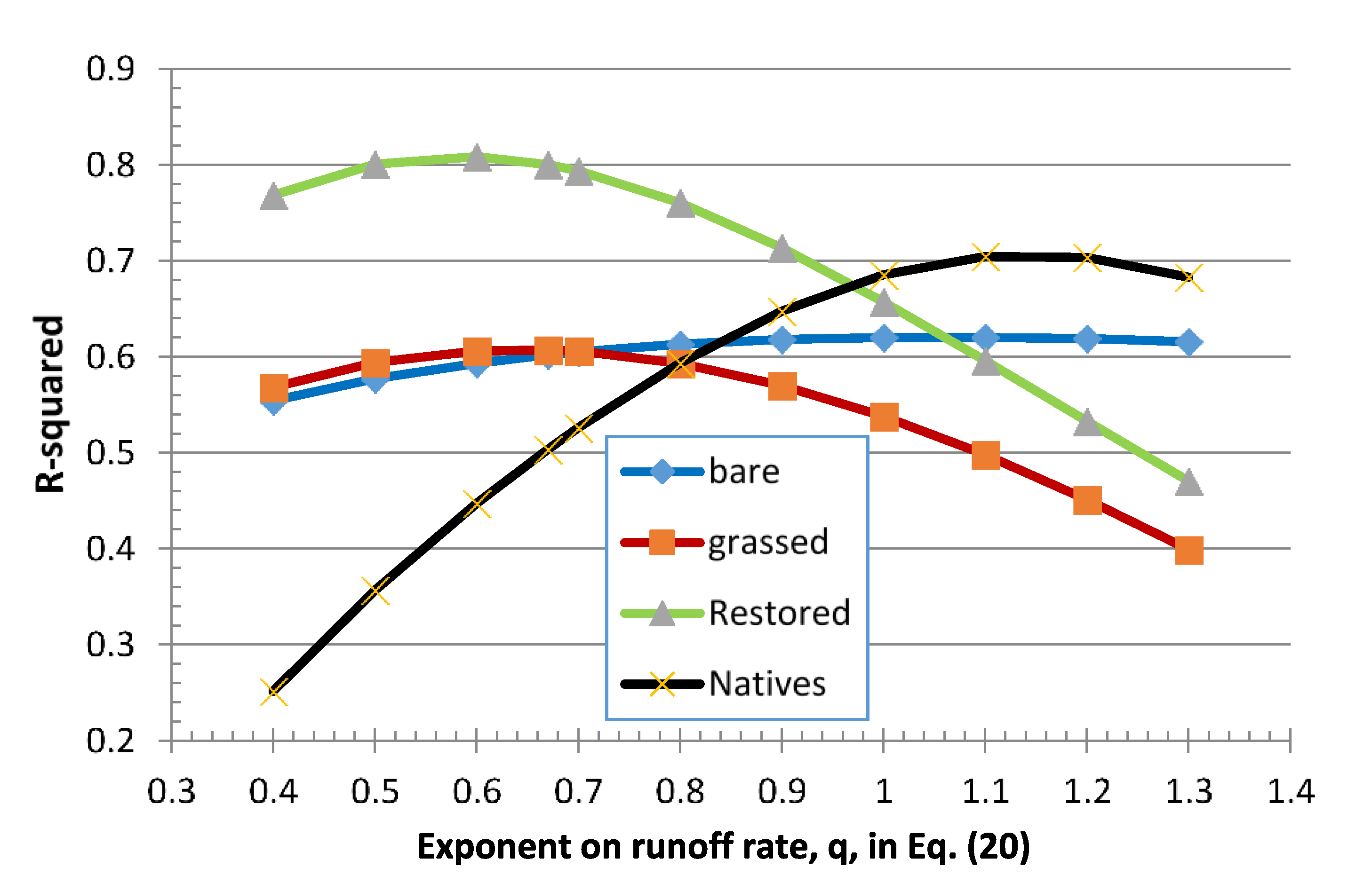
~1.3 and then determine the optimal exponent applicable to the runoff rate.


