Article

Assessing Terrestrial Water Storage Variations in Southern Spain Using Rainfall Estimates and GRACE Data

by
Eulogio Pardo-Igúzquiza
1,*,
Jean-Philippe Montillet
2,3,
José Sánchez-Morales
4,
Peter A. Dowd
5,
Juan Antonio Luque-Espinar
6,
Neda Darbeheshti
7 and
Francisco Javier Rodríguez-Tovar
4
1
Instituto de Geociencias (CSIC-UCM), Severo Ochoa 7, 28040 Madrid, Spain
2
Space and Earth Geodesy Laboratory (SEGAL), Universita da Beira Interior, 6201-001 Covilha, Portugal
3
World Radiation Center (WRC), 7260 Davos, Switzerland
4
Departamento de Estratigrafía y Paleontología, Universidad de Granada, Campus Fuentenueva s/n, 18071 Granada, Spain
5
Faculty of Sciences, Engineering and Technology, University of Adelaide, Adelaide, SA 5005, Australia
6
Instituto Geológico y Minero de España, Urbanización Alcázar del Genil 4, Edificio Zulema, 18006 Granada, Spain
7
Independent Researcher, 1000-001 Lisbon, Portugal
*
Author to whom correspondence should be addressed.
Hydrology 2023, 10(9), 187; https://doi.org/10.3390/hydrology10090187
Submission received: 18 July 2023 / Revised: 11 September 2023 / Accepted: 13 September 2023 / Published: 15 September 2023
(This article belongs to the Section Hydrology–Climate Interactions)

Abstract

:
This paper investigates the relationship between rainfall, groundwater and Gravity Recovery and Climate Experiment (GRACE) data to generate regional-scale estimates of terrestrial water storage variations in the Andalucía region of southern Spain. These estimates can provide information on groundwater depletion (caused by periods of low rainfall or droughts) and groundwater recovery. The spatial distribution of groundwater bodies in southern Spain is complex and current in situ groundwater monitoring methods are deficient, particularly in terms of obtaining representative samples and in implementing and maintaining groundwater monitoring networks. The alternative approach proposed here is to investigate the relationship between precipitation time series and changes in the terrestrial water storage estimated from GRACE observations. The results were validated against the estimated fluctuation in regional groundwater. The maximum correlation between the mean groundwater level and the GRACE observations is 0.69 and this occurs at a lag of one month because the variation in gravity is immediate, but rainfall water requires around one month to travel across the vadose zone before it reaches the groundwater table. Using graphical methods of accumulated deviations from the mean, we show that, in general, groundwater storage follows the smooth, multi-year trends of terrestrial water storage but with less short-term trends; the same is true of rainfall, for which the local trends are more pronounced. There is hysteresis-like behaviour in the variations in terrestrial water storage and in the variations of groundwater. In practical terms, this study shows that, despite the abnormal dryness of the Iberian Peninsula during the 2004–2010 drought, the depleted groundwater storage in Andalucía recovered almost to its pre-drought level by 2016. In addition, groundwater storage and terrestrial water storage show very similar trends but with a delay in the groundwater trend.

1. Introduction

The Gravity Recovery and Climate Experiment (GRACE) and the continuing GRACE-Follow-on (GRACE-FO) are space-based missions [1] designed to measure changes in the Earth’s gravity field (in the form of the geoid) that are directly related to variations in surface mass [2]. International research centres provide estimates of the temporal variation of the Earth’s gravity field derived from GRACE observations in the form of spherical harmonic coefficients (Groupe de Recherche en Geodesie Spatiale, Geo Forchungs Zentrum (Potsdam), Centre for Space Research at the University of Texas Austin) or global mascons (NASA/Jet Propulsion Laboratory). Several websites [3,4] provide variations in the gravity field interpreted as a change in geoid height, equivalent water thickness, and viscoelastic or elastic deformation. In continental areas, variations in the gravity field, after atmospheric corrections, are mainly related to redistributions in continental water storages. These spatial and temporal variations in the surface mass signal are largely the sum of the changes in groundwater, water in the vadose zone, soil moisture and surface water stored in dams, lakes, and the snowpack [5]. Previous studies have shown that the GRACE observations can be used to monitor water mass redistributions at the global scale [6,7,8], the continental scale [9,10], the regional scale [11,12,13] and large aquifer scale [14,15]. For large areas in the mid-latitudes, monthly variations in the snowpack and in water in dams and lakes are small relative to the total terrestrial water storage (TWS). In these cases, the TWS can be regarded as the variation in the water in the subsurface including soil water storage (SWS), groundwater storage (GWS) and water in the vadose zone that can be considered to be in transit from the SWS to the GWS in the groundwater recharge process. Despite the importance of SWS in agriculture and evapotranspiration, GWS is the primary contributor to groundwater resources. GWS can be considered as a deposit from which water can be extracted for irrigation, industrial purposes and potable purposes. Groundwater delivers a worldwide average of 42% of the water required for irrigation [16]. The natural discharge of groundwater gives rise to springs, and it is the origin of rivers that support important aquatic ecosystems [17]. The widespread decline in groundwater levels over recent years [18] is generally associated with higher extraction rates and longer periods of severe drought [19,20]. Reliable forecasting of the availability of water resources requires local and regional information on aquifer properties together with the impact of long dry periods on the water resources of stressed aquifer systems. The over-extraction of groundwater can cause aquifer compaction with accompanying land subsidence and consequent adverse impacts on infrastructure [21]. Despite the importance of groundwater resources, the general quality and extent of monitoring networks makes it very difficult to quantify changes in the level of groundwater at regional scales [22]. There are significant difficulties in processing in situ data such as the extent to which samples are representative of each aquifer; the quality and extent of the maintenance of monitoring networks; the representativeness of piezometers in relation to the spatial variability within a single aquifer; and the cost of sampling in frequency and in space [23]. The use of the GRACE data could circumvent these issues and provide a direct measurement of regional groundwater variation, i.e., depletions and recoveries [20,24], whilst rendering the process more efficient. Van Loon et al. [25] used GRACE observations to study the impact of drought on spatially variable groundwater patterns in Europe. Other studies have used GRACE observations to investigate the manner in which worldwide drought is changing due to climate change [26].
The purpose of the work presented here is to assess the possibility of using GRACE data as a surrogate for groundwater variability over time (depletion and recovery of groundwater resources) at a regional scale and in a region with high hydrogeological complexity. There are many scientific papers using GRACE data in relation to the hydrology of large river basins or large aquifers. The case study presented here is in an administrative area (the Andalucía autonomous region in southern Spain with an area of 87,000 km2) with high hydrogeological complexity. A total of 62% of the surface can be considered as permeable and able to store groundwater (i.e., aquifers) and 38% of the surface can be considered as impervious and without aquifers. Furthermore, the 62% of the permeable surface includes 189 aquifers with complex spatial dispositions. In this context, there is a significant difficulty, if not an impossibility in practical terms, in using in situ measurements to monitor the regional groundwater variations for the entire Andalucía region. The purpose of this paper is to analyse the possibility of monitoring the groundwater evolution (depletion and recoveries) by using the gravity data provided by GRACE.

2. Methodology and Assumptions for the Hydrological Cycle, Rainfall Data and GRACE Observations

The ANU GRACE visualisation tool portal [3], based on the spherical harmonics field estimated by the Groupe de Recherche en Geodesie Spatiale (GRGS), was used to estimate the equivalent water height or terrestrial water storage (TWS) time series at specific locations. The TWS time series were estimated using the integrated water change equation [3,5]:
Δ T W S ( θ , λ , t ) = l = 2 L m = 0 l R ρ e 3 ρ w 2 l + 1 1 + k l P l m ( cos ( θ ) ) [ Δ C l m cos ( m λ ) + Δ S l m sin ( m λ ) ] ,
where Δ T W S ( θ , λ , t ) represents the variation in terrestrial water storage at the geographical location of co-latitude ( θ ) and longitude ( λ ) at time ( t ) ; R is the radius of the Earth; l , m are, respectively, the degree and order of the spherical harmonic model; P l m ( cos ( θ ) ) is the normalised associated Legendre functions at co-latitude ( θ ) ;   ρ e and ρ w are, respectively, the densities of the Earth and water; k l is the elastic load Love numbers of degree l ; and Δ C l m and Δ S l m are the spherical harmonic coefficient anomalies from the GRGS GRACE gravity fields at time ( t ) . This equation is a function of the spherical harmonic coefficients and the maximum harmonic degree (L) of the spherical harmonic expansion. This parameter is important in gravity field recovery and, depending on the geographical location, an increase or decrease in its value impacts not only the stochastic noise properties of the resulting time series but may also result in the inclusion of other gravity effects from mass concentrations that are outside the spatial region that the measure represents, a phenomenon known as spatial gravity leakage [27,28]. A rough estimate of the spatial resolution (SR) is given by the relationship S R = π / L [29], which implies that the GRACE measurement at a given location refers to an average value over a square area of side-length 680 km for degree 30 and of 400 km for degree 50. Using geostatistical terminology [30], this area is termed the spatial support of the GRACE data. In the same manner, the time support of the GRACE data is a month because the data are monthly accumulations of gravity anomalies.
The uncertainties of the computed TWS values were calculated using the method of propagating the variances by the following equation [3] that uses the methodology of propagation of errors [31]:
σ T W S 2 ( t ) = σ Δ C ( t ) 2 ( T W S Δ C ( t ) ) 2 + σ Δ S ( t ) 2 ( T W S Δ S ( t ) ) 2
where σ T W S 2 ,   σ Δ C ( t ) 2 ,   σ Δ S ( t ) 2 are the variances of TWS, Δ C ( t )   and   Δ S ( t )   , respectively. Usually, for each Δ T W S ( θ , λ , t ) there is an associated uncertainty that is evaluated by σ T W S ( t ) , the standard error or standard deviation from Equation (2), which in general is of the order of 1 to 2 cm [3]. A recent study of the uncertainty evaluation of GRACE data can be found in Boergens et al. [32]. The uncertainty of the data used in the case study presented in this paper is discussed below.
One advantage of the GRGS spherical harmonic models is that they are generated in a way that does not require any filtering (i.e., spatial smoothing) or decorrelation (i.e., de-striping) steps [33,34,35] before using the data [3]. Some of the GRACE products use various techniques to filter the raw gravity observations recorded by satellites. We compared the results obtained for the CNES-GRGS data with those of the Centre for Space Research (CSR) at the University of Texas Austin [36] and retrieved from the EGSIEM website [4] and the results were similar.
A TWS time series is a function of the change in the Earth’s gravity field due to changes in mass load, in general, water. In other words, it is the variation of the sum of terrestrial water storage that can be decomposed into surface water storage (SWS), soil moisture storage (SMS) and groundwater storage (GWS) after rainfalls in the wet season (Figure 1A). However, in the dry season, the variation in TWS is mainly proportional to GWS (Figure 1B). Water input to the system comes from precipitation (P in Figure 1A), which may be in the form of liquid water (rainfall) or solid-state water (snow water equivalent, SWE); the latter can be seasonally accumulated in snowpacks in mountainous areas. The SWE and water stored in dams (D), lakes, wetlands and other repositories are the main components of SWS. SMS is the water stored in soil and, after accounting for evapotranspiration (ET), if the maximum storage value is exceeded, the excess water percolates and travels across the vadose zone until it reaches the groundwater zone (i.e., the recharge process). Water from rainfall enters the soil up to an infiltration value and the excess runs over the landscape (runoff water, R), entering drainage channels and forming streams that appear after a rainfall event. In the wet season, there is a transit of water across the vadose zone (VZ) from the soil zone (SZ) to the saturated zone or proper groundwater zone (SGZ). In the dry season (Figure 1B), the main contribution to the loss of TWS is from the decreasing GWS. This suggests a hysteresis-like behaviour of the GRACE signal in which the GWS lags behind the TWS and there is an obvious larger variability in the humid periods than in the dry periods.
Following [37] and our description of the water storage, the hydrological cycle and water budget can be written as:
P = R + E T + Δ S W S + Δ S M S + Δ G W S ,  
where P is the total precipitation, R is runoff, ET is evapotranspiration, Δ SWS is the variation in SWS, Δ SMS is the variation in SMS and Δ GWS is the variation in GWS. After rainfall in the wet season, it is assumed that Δ SWS, Δ SMS and Δ GWS increase. In the dry season (Figure 1B) there is a decrease in Δ SWS, Δ SMS and Δ GWS, with the latter being the most significant. Then, the water flowing in rivers in the dry season comes from aquifer discharge from the GWS.
Thus,
Δ T W S = Δ S W S + Δ S M S + Δ G W S ,
and therefore
P = R + E T + Δ T W S .  
There is also the gravity or GRACE data and, as the GRGS gravity field variation ( Δ G F ) was corrected for changes in atmospheric and ocean variations [3], it is directly proportional to the variation in TWS:
Δ G F Δ T W S .
Thus, during the wet season:
Δ G F Δ S W S + Δ S M S + Δ G W S .  
whereas during the dry season the TWS is mainly groundwater and thus:
Δ G F Δ G W S ,
The same reasoning can be extended from the yearly dry and wet seasons to a continuous multi-annual period of dry years with below-average rainfall (drought conditions) and to a multi-annual period of wet years (humid conditions with above average rainfall). Thus, in the variation in the gravity field, the effect lags behind its cause with more variability in the humid periods and less variability in the drought periods. During drought conditions, there is a decrease in groundwater storage that may be recovered during humid periods. However, it is possible that the rainfall in the humid periods may not be sufficient to recover to pre-drought levels, leading to aquifer depletion.
A useful tool in this study was the cumulative departure from the mean statistic [38] used to enhance the correlation in the short-term trends of rainfall data and TWS. Previous work, such as [38], studied the validity of the cumulative rainfall departure (CRD) and concluded that the CRD is a useful indicator of short-term rainfall trends and is an important parameter for the remainder of this paper. Given a set of n rainfall measurements { R 1 , R 2 , , R n } with mean value:
R ¯ = 1 n i = 1 n R i ,    
the CRD is defined as:
C R D ( k ) = i = 1 k ( R i R ¯ ) .
To ensure a meaningful comparison of the two datasets in the following case study, the same concept of cumulative departures from the mean statistic (CDMS) was applied to the TWS measurements and to the groundwater heads in the validation stage:
C D M S ( k ) = i = 1 k ( T W S i T W S ¯ ) ,  
where T W S ¯ is the mean value of the TWS measurements T W S i . The CDMS can be applied to the time series of any other variable.

3. Case Study: The Andalucía Region of Southern Spain

The study area is in the Andalucía region of southern Spain as shown in Figure 2, which has an area of 87,000 km2. This region is known for its high rainfall variability and includes the low-rainfall areas in the east and high-rainfall areas in the southwest. In Andalucía, dry periods can adversely impact non-irrigated crops (e.g., olive trees), especially in years when abnormally low rainfalls induce severe droughts, for example, the exceptional drought in south-eastern Spain from October 2013 to July 2014 [39]. Eight geographical locations, shown in Figure 2 as large purple dots, were defined on a rectangular grid of 180 km × 90 km covering this region. The geographical co-ordinates of the grid points are shown in Table 1. Because the GRACE measurement at each point represents the mean value of a very large area (for example a square of 400 km × 400 km for maximum degree L = 50 in the spherical harmonics), the measurements overlap and it is irrelevant whether the grid was arbitrarily chosen, as the same results would be obtained with similar alternative grids. Figure 2 also shows a grid (small purple dots) of 5 km × 5 km covering the region of Andalucía that was used to obtain the rainfall estimates as explained below. The monthly TWS time series, for maximum degrees of L = 30 and L = 50, estimated at location 7 from the GRACE observations are shown in Figure 3A. Figure 3 shows 152 values, of which 144 are original GRACE data and the 8 missing monthly values were obtained by linear interpolation from their two nearest neighbours. The reason for the missing values is the failure of the satellite instruments. The completion of the GRACE time series was not strictly necessary for the purposes of this paper, but it was performed for completeness and for calculating the CDMS. It should be noted that these time series represent the average monthly accumulated variations in the gravity field for square areas of side lengths 680 km and 400 km for maximum spherical harmonic degrees L = 30 and L = 50, respectively. In particular, for the period of the anomalies below the average (dry periods denoted by (a) in Figure 3A), the peaks of the valleys are more negative, whereas during the period of anomalies above the average (humid periods, denoted by (b) in Figure 3A), the peaks of the annual maximum are higher. Nevertheless, the 0.90 coefficient of correlation between the two time series is high. Figure 3B shows, for the same maximum degree L = 50, the TWS time series for locations 6 and 7 in Figure 2. The two time-series are very similar (coefficient of correlation of 0.91) because there is a significant overlap of the spatial support of the measurements of two 400 km × 400 km areas, the centres of which are separated by 180 km. This is the conventional 400 km scale [40], which is adequate for studies of the water storage of large structures such as river basins [41], large aquifers [20], and areas with many aquifers and aquicludes as shown below. As the maximum degree of the spherical harmonics (L) increases, the spatial resolution increases (i.e., the support or area decreases) and the variability increases. As can be seen in Figure 3C for location 7a, the uncertainty of the GRACE TWS estimates also increases as the maximum number L of spherical harmonics in Equation (1) increases. In Figure 3C, the uncertainty is evaluated as the square root of the error variance of Equation (2), that is, the standard error or standard deviation of the error. The mean of the errors are 10 mm, 25 mm and 150 mm for the maximum degree of the spherical harmonics of L = 30, L = 50 and L = 80, respectively. While the standard error is acceptable for L = 30 and for L = 50, the standard error for L = 80 is so large that it renders the GRACE data almost useless and, thus, is not used in the work presented here. Figure 3C also shows the variability of the standard errors around their mean values and sometimes there is a spike in the time series, that is, a particularly high uncertainty value for a given month. The magnitude of the standard error is not correlated with the magnitude of the GRACE TWS data. The origin of these spikes may be due to the cumulative uncertainty in different GRACE instruments in that specific months possibly generating computational errors. Figure 3D shows a new perspective of Figure 3B obtained by considering the uncertainty of the measurements. The latter figure shows, for the same maximum degree L = 50, the TWS time series for locations 6 and 7 (as in Figure 3B) plus the standard error of the TWS for the location. This figure shows that the TWS of location 6 is within the interval of the TWS  ± 1 standard error of location 7. In addition, the uncertainty for locations 6 and 7 is almost the same if the same maximum degree L is considered for both locations.
Rainfall estimates on a 5 km × 5 km grid for the Andalucía test site were obtained from the Agencia Estatal de Meteorología (Spanish Meteorological Office (www.ign.es) accessed on 30 March 2022). Temperature estimates on a 10 km × 10 km grid were retrieved from the Spain02 climate database [42]. The mean rainfall values over the test area from 2002 to 2015, the period in which the original GRACE data were recorded, were obtained by averaging the rainfall estimates on the 5 km × 5 km grid. The mean surface temperatures for the same time period were obtained by averaging the mean temperature estimates from the 10 km × 10 km grid.

4. Analysis and Discussion of the Results

The areal monthly rainfall estimates for a 200 km × 200 km area centred on location 7 (red square in Figure 1) and for the whole of Andalucía (small purple dots in Figure 1) are shown in Figure 4A. These estimates show that, for large areas, whilst the variability in the rainfall time series is similar, the magnitudes are different. In Figure 4B, these rainfall estimates are compared with the TWS time series from GRACE for maximum degree L = 50, from which it can be concluded that, in general, the GRACE signal for maximum degree L = 50 captures the bimodality of rainfall together with other small variations that can be attributed to noise or to the filtering technique applied to the raw gravity field [36]. They may also be the result of spatial leakage, a major limitation on the quantitative interpretation of satellite gravity measurements at regional scales. The latter phenomenon has been well documented over the past decade [40,43]. Thus, in assessing the variation in TWS, the GRACE signal for maximum degree L = 30 (Figure 3A) is used when smoother variation is required and the signal for maximum degree L = 50 is used when the bimodality of each annual cycle is required. In addition, it is evident that for several peaks in Figure 4B there is a delay of around one to two months between the TWS time series and the rainfall data. This delay has been noted in various studies, e.g., [20,44], and is caused by the GRACE data registering the gravity anomalies introduced by the mass of water supplied by rainfall stored on the surface or underground. In other words, the TWS time series is derived from rainfall and if the rainfall data were a perfect sinusoid, the TWS signal (a cosine obtained by a 90° horizontal shift) would have a delay of 90°, or a quarter of the three-month wavelength. Figure 5 shows the TWS time series estimated with GRACE data at maximum degree L = 50, together with the mean surface temperature. The two curves are in opposite phase. The correspondence between minimum temperature and maximum TWS, and the reverse, is a consequence of rainy seasons that occur in winter and spring and dry seasons that occur during the summer and early autumn.
A spectral analysis using the Lomb–Scargle periodogram [45] was used to check the cyclical signal recorded in the TWS and the rainfall data. The Lomb–Scargle periodogram is specially designed for the spectral analysis of time series with uneven spacing of the observations such as the TWS time series where there are missing data. This avoids the artefacts introduced in the estimated spectral functions when the time series are completed by interpolation to yield even time series. The estimated periodogram is shown in Figure 6A in which the main cyclicities are highlighted. The annual hydrological cycle is evident, with the most prominent peak for a one-year period. The wet season in the study area is bimodal [46], meaning that it appears to have an almost half-year cycle with peaks at 5.4 months due to the variability of the bimodality changing from year to year. Figure 6A also shows longer cycles of 3.2 and 11.9 years. Some studies have discussed the relationship between the 3.2-year cycle and the North Atlantic Oscillation phenomenon [47]. The 11.9-year cycle may be related to the North Atlantic Oscillation cycle in the six to ten-year range [48] or with the 11-year sunspot cycle. The time series are too short to draw any conclusive conclusions. Comparable peaks can be seen in the GRACE data and the rainfall data. The relationship between the TWS time series and rainfall is clear from the cross-spectral analysis as shown in [45]. The squared coherence plots in Figure 6B show high-value peaks (the maximum value of the squared coherence is 1) at frequencies that correspond to periods of 3.6 years, 1 year and 7.8 months. The statistical confidence levels of these coherence values shown in Figure 6C were evaluated using the permutation test [45]. The estimated phases are shown in Figure 6D in which the phases of 3.6 years, 1 year and 7.8 months as periodicities have values of 55°, 27° and 24°, respectively, which imply delays between TWS and rainfall of 6.6 months, 1 month and 0.5 months, respectively. While the 1 month or 1.5-month delays are visually evident in Figure 4B, the delay of almost 7 months implies a delay in the trends of the signals as discussed below.
The general and local trends for the CRD and the accumulated TWS time series for maximum degree L = 50 and location 7 are shown in Figure 7. The results show a possible short increasing trend between (a) and (b) followed by a significant negative slope between (b) and (c) and a significant positive slope between (c) and (e). The variations in the accumulated TWS time series are smoother than those of the rainfall data. The TWS time series has more inertia, i.e., less variability and a smoother response, than the large oscillations in rainfall, although both variables show the same trend. Rainfall, in particular, includes the runoff water mass and evapotranspiration that are not included in the TWS variations. Assuming the variations in the gravity field recorded in Andalucía are mostly related to GWS levels, the minimum CRD and the accumulated TWS in (c) around the end of 2010 must have resulted in minimum GWS in the area, which is verified below. Figure 7 clearly shows the significant drought in Andalucía that started in 2004 and ended in 2010 (Junta de Andalucía, Medio Ambiente, http://www.juntadeandalucia.es/medioambiente/(accessed on 30 March 2022)). It also shows that, by 2016, the rainfall since 2010 allowed the depleted GWS to recover to a level almost comparable to that of the pre-drought period. According to [49], the southern half of the Iberian Peninsula received less than 40% of its usual precipitation by June 2005, with the consequent depletion of large aquifers in the peninsula [50].
The value of the TWS provided by GRACE can only be fully appreciated by considering the difficulty in estimating the state of the groundwater resources at the regional level of the Andalucía region (Figure 1). Figure 8 shows the distribution of groundwater bodies. Each groundwater body may comprise a single aquifer or several aquifers. In Figure 8, it is also possible to see large zones of low permeability (aquicludes). There is thus a problem in monitoring groundwater levels across a region with a high number of groundwater bodies and aquicludes. An expert selection of eleven piezometers, which are generally considered representative of the natural behaviour of the corresponding aquifers and are not affected by pumping, are shown as solid black dots in Figure 8. For illustrative purposes, Figure 9 shows the evolution of water heads for four of these piezometers. The groundwater variability was estimated as the difference between each water-head time series and its mean followed by averaging the eleven time series. In addition, the time series was rescaled as an anomaly with respect to the period 2004–2009, which is the period to which GRACE data are usually referred. The time series of the anomalies are shown in Figure 10. The rainfall and TWS (GRACE, maximum degree L = 30) time series are referred to the same baseline to calculate the anomalies. The accumulated differences with respect to the mean are shown in Figure 11 together with the accumulated differences with respect to the mean for the groundwater time series in Figure 10. This Figure shows that the groundwater time series register the multi-year trends, and their behaviour is much smoother with respect to the rainfall and TWS time series, which also register the same trends together with other short-range trends as discussed in relation to Figure 7. The groundwater levels begin to decrease in 2005, and the minimum is reached in 2010, followed by recovery.
The groundwater time series and the TWS data and rainfall data are compared further in Figure 12. Figure 12A shows good agreement between the evolution of the TWS anomalies and the groundwater anomalies with a delay in the peaks. The delay is because the TWS anomaly is due to an excess of water mass that includes the water in the soil and in the vadose zone prior to the recharge; this reaches the water table at the end of the recharge, thus affecting the groundwater level. The figure includes the coefficient of correlation and the values of the correlation function of different lags, where lag 1 is equal to one month and lag 2 is equal to two months. The coefficient of correlation is the correlation function for lag 0. The maximum correlation is for lag 1 and is equal to 0.69. Thus, there is an average time delay of one month between the gravity signal and the groundwater level because of the previously explained traveling time of the part of the rainfall water that, infiltrated into the soil, must travel across the vadose zone until it reaches the groundwater table. The effects of this traveling water on gravity are instantaneous, but they can only be detected by in situ monitoring when they arrive and increase the groundwater level.
Figure 12B compares the rainfall anomalies and the groundwater anomalies and the same delay, for the same reasons, is evident between the peaks. There must be a positive rainfall anomaly (humid period) if the groundwater levels recover, whereas there must be a negative rainfall anomaly (drought) if the groundwater levels decrease. Figure 12C compares the TWS anomalies and the rainfall anomalies from which similar conclusions can be drawn to those in the discussion of Figure 4B.
Finally, the long-term trend between TWS and GWS (groundwater heads) was assessed by filtering the annual trend using a moving average filter with a half-bandwidth of 12 months. The result of the filtering is shown in Figure 13, which clearly shows that the GWS trend is a delayed version of the TWS. Thus, the TWS can be used to monitor the GWS of the Andalucía region. This is a significant outcome for a region that has a complex distribution of aquifers and aquicludes and very limited monitoring.

5. Conclusions

The hypothesis considered in this work is that GRACE observations and, in particular, the TWS time series, provide a means of investigating the regional evolution of groundwater resources based on rainfall estimates and, for the target region, most of the TWS signal is determined by variations in groundwater. The relationship between the TWS time series and rainfall data was analysed in detail. Using the accumulated rainfall differences and the accumulated TWS curves, our hypothesis is supported by the correlation between rainfall and the TWS time series in terms of temporal trends as shown graphically in Figure 7. More importantly, there is good correlation (numerical values in Figure 12A) between the mean groundwater and TWS. The cumulated differences of the TWS time series show that the GWS depletion over the long drought from 2004 to 2010 mostly been recovered by 2016. Furthermore, the estimated regional groundwater variation validates the previous findings and shows that the GRACE TWS is a smooth version of rainfall and, in turn, the groundwater is a smooth version of the TWS. TWS shows hysteresis-like behaviour between drought periods and humid periods. Our analyses of the periodogram of the rainfall and of the TWS time series show similar peaks at known frequencies representing cyclicities related to seasonal cycles and climate events (e.g., NAO phenomenon, sunspot cycles). Finally, we show that the pluri-annual GWS trend is a delayed version of the TWS trend, and thus the filtered GWS time series can be used as a surrogate of the state of the groundwater resource, its depletion, and its recoveries without the need for an exhaustive monitoring network. It is unlikely that such a network will ever be implemented in this region (and in many other similar regions around the world) because of the costs of design, implementation, maintenance and the routine collection of measurements at piezometer sites.

Author Contributions

Conceptualization, E.P.-I. and J.-P.M.; methodologyanalysis, J.S.-M. and F.J.R.-T.; results validation, E.P.-I., J.A.L.-E., N.D. and P.A.D.; writing—original draft preparation, E.P.-I. and J.-P.M.; writing—review and editing, E.P.-I., J.-P.M.; and P.A.D.; visualisation, E.P.-I. and J.S.-M. All authors have read and agreed to the published version of the manuscript.

Funding

Funding for this research was provided by Projects PID2019-106435GB-I00 (Ministerio de Ciencia e Innovación) and CGL2015-66835-P (Ministerio de Ciencia, Innovación y Universidades).

Data Availability Statement

The data are freely available under request from the corresponding author.

Acknowledgments

We thank the three anonymous reviewers who provided constructive comments that allowed us to improve the final version of this paper.

Conflicts of Interest

The authors declare no conflict of interest. The authors declare that they have no known competing financial interests or personal relationships that could have appeared to influence the work reported in this paper.

Abbreviations

The following list describes, in alphabetic order, the acronyms used in this paper.
CDMSCumulative departures from the mean statistic
CRDCumulative rainfall departure
CSRCentre for Space Research
DWater stored in dams
EGSIEMEuropean Gravity Service for Improved Emergency Management
ETEvapotranspiration
GdGroundwater discharge
GFGravity field
GRACEGravity Recovery and Climate Experiment
GRACE-FOGravity Recovery and Climate Experiment Follow-on
GRGSGroupe de Recherche en Geodesie Spatiale
GWSGroundwater storage
IInfiltration water
LMaximum harmonic degree of the spherical harmonic expansion of the geoid
NAONorth Atlantic Oscillation
PPrecipitation water
RRunoff water
SEStandard error or standard deviation (square root of the error variance)
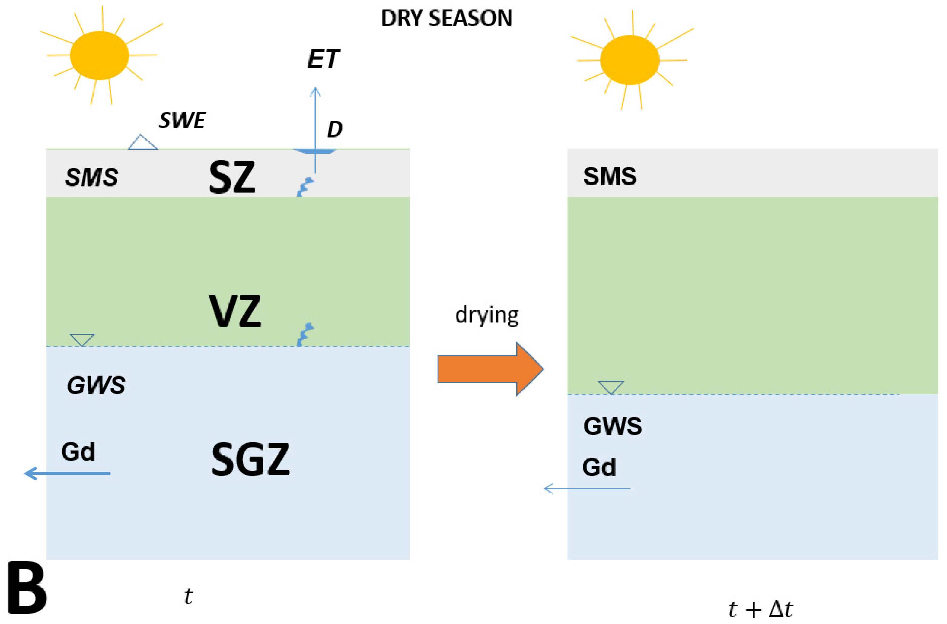
SGZGroundwater zone or saturated zone
SRSpatial resolution
SZSoil zone
SWESnow water equivalent
SWSSoil water storage
TWSTerrestrial water storage
VZVadose zone

References

  1. Darbeheshti, N.; Wöske, F.; Weigelt, M.; Wu, H.; Mccullough, C. Comparison of Spacewise and Timewise Methods for GRACE Gravity Field Recovery. In Geodetic Time Series Analysis in Earth Sciences; Montillet, J.P., Bos, M., Eds.; Springer Geophysics; Springer: Cham, Switzerland, 2020. [Google Scholar] [CrossRef]
  2. Tapley, B.D.; Bettadpur, S.; Watkins, M.; Reigber, C. The gravity recovery and climate experiment: Mission overview and early results. Geophys. Res. Lett. 2004, 31, L09607. [Google Scholar] [CrossRef]
  3. Darbeheshti, N.; Zhou, L.; Tregoning, P.; McClusky, S.; Purcell, A. The ANU GRACE visualization web portal. Comput. Geosci. 2013, 52, 227–233. [Google Scholar] [CrossRef]
  4. EGSIEM. European Gravity Service for Improved Emergency Management Report No. 11. 2018. Available online: http://www.egsiem.eu/images/Newsletters/EGSIEM_newsletter_no_11.pdf (accessed on 30 March 2022).
  5. Wahr, J.; Molenaar, M.; Bryan, F. Time variability of the Earth’s gravity field: Hydrological and oceanic effects and their possible detec-tion using GRACE. J. Geophys. Res. 1998, 30, 205–229. [Google Scholar] [CrossRef]
  6. Seo, K.W.; Wilson, C.R.; Famiglietti, J.S.; Chen, J.L.; Rodell, M. Terrestrial water mass load changes from Gravity Recovery and Climate Experiment (GRACE). Water Resour. Res. 2006, 42, W05417. [Google Scholar] [CrossRef]
  7. Landerer, F.W.; Swenson, S.C. Accuracy of scaled GRACE terrestrial water storage estimates. Water Resour. Res. 2012, 48, W04531. [Google Scholar] [CrossRef]
  8. Frappart, F.; Ramillien, G. Monitoring Groundwater Storage Changes Using the Gravity Recovery and Climate Experiment (GRACE) Satellite Mission: A Review. Remote Sens. 2018, 10, 829. [Google Scholar] [CrossRef]
  9. Rodell, M.; Famiglietti, J.S. An analysis of terrestrial water storage variations in Illinois with implications for the Gravity Recovery and Climate Experiment (GRACE). Water Resour. Res. 2001, 37, 1327–1339. [Google Scholar] [CrossRef]
  10. García-García, D.; Ummenhofer, C.C.; Zlotnicki, V. Australian water mass variations from GRACE data linked to Indo-Pacific climate variability. Remote Sens. Environ. 2011, 115, 2175–2183. [Google Scholar] [CrossRef]
  11. Longuevergne, L.; Scanlon, B.R.; Wilson, C.R. GRACE Hydrological estimates for small basins: Evaluating processing approaches on the High Plains Aquifer, USA. Water Resour. Res. 2011, 46, W11517. [Google Scholar] [CrossRef]
  12. Shamsudduha, M.; Taylor, R.G.; Longuevergne, L. Monitoring groundwater storage changes in the highly seasonal humid tropics: Validation of GRACE measurements in the Bengal Basin. Water Resour. Res. 2012, 48, W02508. [Google Scholar] [CrossRef]
  13. Alshehri, F.; Mohamed, A. Analysis of Groundwater Storage Fluctuations Using GRACE and Remote Sensing Data in Wadi As-Sirhan, Northern Saudi Arabia. Water 2023, 15, 282. [Google Scholar] [CrossRef]
  14. Rodell, M.; Famiglietti, J.S. The potential for satellite-based monitoring of groundwater storage changes using GRACE: The High Plains aquifer, Central US. J. Hydrol. 2002, 263, 245–256. [Google Scholar] [CrossRef]
  15. Strassberg, G.; Scanlon, B.R.; Rodell, M. Comparison of seasonal terrestrial water storage variations from GRACE with groundwater-level measurements from the High Plains Aquifer (USA). Geophys. Res. Lett. 2007, 34, L14402. [Google Scholar] [CrossRef]
  16. Döll, P.; Hoffmann-Dobrev, H.; Portmann, F.T.; Siebert, S.; Eicker, A.; Rodell, M.; Strassberg, G.; Scanlon, B.R. Impact of water withdrawals from groundwater and surface water on continental water storage variations. J. Geodyn. 2012, 59, 143–156. [Google Scholar] [CrossRef]
  17. Taylor, R.G.; Scanlon, B.; Döll, P.; Rodell, M.; Van Beek, R.; Wada, Y.; Longuevergne, L.; Leblanc, M.; Famiglietti, J.S.; Edmunds, M.; et al. Ground water and climate change. Nat. Clim. Chang. 2013, 3, 322–329. [Google Scholar] [CrossRef]
  18. Russo, T.A.; Lall, U. Depletion and response of deep groundwater to climate-induced pumping variability. Nat. Geosci. 2017, 10, 105–108. [Google Scholar] [CrossRef]
  19. Farr, T.G.; Jones, C.; Liu, Z. Progress Report: Subsidence in the Central Valley, California. 2015. Available online: https://cawaterlibrary.net/wp-content/uploads/2017/05/JPL-subsidence-report-final-for-public-dec-2016.pdf (accessed on 14 September 2015).
  20. Miller, M.M.; Shirzaei, M.; Argus, D. Aquifer mechanical properties and decelerated compaction in Tucson, Arizona. J. Geophys. Res. Solid Earth 2017, 122, 8402–8416. [Google Scholar] [CrossRef]
  21. Galloway, D.L.; Burbey, T.J. Review: Regional land subsidence accompanying groundwater extraction. Hydrogeol. J. 2011, 19, 1459–1486. [Google Scholar] [CrossRef]
  22. Famiglietti, J.S.; Lo, M.; Ho, S.L.; Bethune, J.; Anderson, K.J.; Syed, T.H.; Swenson, S.C.; de Linage, C.R.; Rodell, M. Satellites measure recent rates of groundwater depletion in California’s Central Valley. Geophys. Res. Lett. 2011, 38, L03403. [Google Scholar] [CrossRef]
  23. Gorelick, S.M.; Zheng, C. Global Change and the Groundwater Management Challenge. Water Resour. Res. 2015, 51, 3031–3051. [Google Scholar] [CrossRef]
  24. Richey, A.S.; Thomas, B.F.; Lo, M.H.; Reager, J.T.; Famiglietti, J.S.; Voss, K.; Swenson, S.; Rodell, M. Quantifying renewable groundwater stress with GRACE. Water Resour. Res. 2005, 51, 5217–5238. [Google Scholar] [CrossRef] [PubMed]
  25. Van Loon, A.F.; Kumar, R.; Mishra, V. Testing the use of standardized indices and GRACE satellite data to estimate the European 2015 groundwater drought in near-real time. Hydrol. Earth Syst. Sci. 2017, 21, 1947–1971. [Google Scholar] [CrossRef]
  26. Tapley, B.D.; Watkins, M.M.; Flechtner, F.; Reigber, C.; Bettadpur, S.; Rodell, M.; Sasgen, I.; Famiglietti, J.S.; Landerer, F.W.; Chambers, D.P.; et al. Contributions of GRACE to Understanding Climate Change. Nat. Clim. Chang. 2019, 9, 358–369. [Google Scholar] [CrossRef] [PubMed]
  27. Lemoine, J.-M.; Bourgogne, S.; Bruinsma, S.; Gégout, P.; Reinquin, F.; Biancale, R. GRACE RL03-v2 Monthly Time Series of Solutions from CNES/GRGS; European Geosciences Union: Vienna, Austria, 2015; id. 1 4461.
  28. Seo, K.-W.; Oh, S.; Eom, J.; Chen, J.; Wilson, C.R. Constrained Linear Deconvolution of GRACE Anomalies to Correct Spatial Leakage. Remote Sens. 2020, 12, 1798. [Google Scholar] [CrossRef]
  29. Vishwakarma, B.D.; Devaraju, B.; Sneeuw, N. What is the spatial resolution of GRACE satellite products in Hydrology? Remote Sens. 2018, 10, 852. [Google Scholar] [CrossRef]
  30. Chilès, J.-P.; Delfiner, P. Geostatistics: Modeling Spatial Uncertainty, 2nd ed.; Wiley: Hoboken, NJ, USA, 2012; 699p. [Google Scholar]
  31. Bevington, P.R.; Robinson, D.K. Data Reduction and Error Analysis for The Physical Sciences, 2nd ed.; WCB-McGraw-Hill: New York, NY, USA, 1996; 328p. [Google Scholar]
  32. Boergens, E.; Kvas, A.; Eicker, A.; Dobslaw, H.; Schawohl, L.; Dahle, C.; Murböck, M.; Flechtner, F. Uncertainties of GRACE-based terrestrial water storage anomalies for arbitrary averaging regions. J. Geophys. Res. Solid Earth 2022, 127, e2021JB022081. [Google Scholar] [CrossRef]
  33. Swenson, S.; Wahr, J. Post-processing removal of correlated errors in GRACE data. Geophys. Res. Lett. 2006, 33, L08402. [Google Scholar] [CrossRef]
  34. Chen, J.L.; Wilson, C.R.; Famiglietti, J.S.; Rodell, M. Attenuation effect on seasonal basin-scale water storage changes from GRACE time-variable gravity. J. Geod. 2007, 81, 237–245. [Google Scholar] [CrossRef]
  35. Bruinsma, S.; Lemoine, J.-M.; Biancale, R.; Valès, N. CNES/GRGS 10-day gravity field models release 2 and their evaluation. Adv. Space Res. 2010, 45, 587–601. [Google Scholar] [CrossRef]
  36. Save, H.; Bettadpur, S.; Tapley, B.D. High resolution CSR GRACE RL05 mascons. J. Geophys. Res. Solid Earth 2016, 121, 7547–7569. [Google Scholar] [CrossRef]
  37. Narasimhan, T. Hydrological Cycle Water Budgets in the Encyclopedia of Inland Waters; Likens, G.E., Ed.; Elsevier: Amsterdam, The Netherlands, 2009. [Google Scholar]
  38. Weber, K.; Stewart, M. A critical analysis of the cumulative rainfall departure concept. Ground Water 2004, 42, 935–938. [Google Scholar]
  39. Micale, F.; Cammalleri, C. Drought News August 2014, Report from the European Drought Observatory. 2014. Available online: https://edo.jrc.ec.europa.eu/documents/news/EDODroughtNews201408.pdf (accessed on 30 March 2022).
  40. Jin, S.; Zou, F. Re-Estimation of Glacier Mass Loss in Greenland from GRACE with Correction of Land-Ocean Leakage Effects. Glob. Planet. Chang. 2015, 135, 170–178. [Google Scholar] [CrossRef]
  41. Reager, J.T.; Famiglietti, J.S. Characteristic mega-basin water storage behavior using GRACE. Water Resour. Res. 2013, 49, 3314–3329. [Google Scholar] [CrossRef]
  42. Herrera, S.; Gutiérrez, J.M.; Ancell, R.; Pons, M.R.; Frías, M.D.; Fernández, J. Development and Analysis of a 50-year high-resolution daily gridded precipitation dataset over Spain (Spain02). Int. J. Climatol. 2012, 32, 74–85. [Google Scholar] [CrossRef]
  43. Chen, J.L.; Wilson, C.R.; Li, J.; Zhang, Z. Reducing Leakage Error in GRACE-Observed Long-Term Ice Mass Change. J. Geod. 2015, 89, 925–940. [Google Scholar] [CrossRef]
  44. Ospina, D.L.; Vargas, C.A. Monitoring runoff coefficients and groundwater levels using data from GRACE, GLDAS, and hydrometeorological stations: Analysis of a Colombian foreland basin. Hydrogeol. J. 2018, 26, 2769–2779. [Google Scholar] [CrossRef]
  45. Pardo-Igúzquiza, E.; Rodríguez-Tovar, F.J. Spectral and cross-spectral analysis of uneven time series with the smoothed Lomb-Scargle periodogram and Monte Carlo evaluation of statistical significance. Comput. Geosci. 2012, 49, 207–216. [Google Scholar] [CrossRef]
  46. Sumner, G.; Homar, V.; Ramis, C. Precipitation seasonality in eastern and southern coastal Spain. Int. J. Climatol. 2001, 21, 219–247. [Google Scholar] [CrossRef]
  47. Pozo-Vázquez, D.; Esteban-Parra, M.J.; Rodrigo, F.S.; Castro-Díez, Y. An analysis of the variability of the North Atlantic Oscillation in the time and the frequency domains. Int. J. Climatol. 2000, 20, 1675–1692. [Google Scholar] [CrossRef]
  48. Hurrell, J.M.; van Loon, H. Decadal variations in climate associated with the North Atlantic Oscillation. Clim. Chang. 1997, 36, 301–326. [Google Scholar] [CrossRef]
  49. García-Herrera, R.; Paredes, D.; Trigo, R.M.; Trigo, I.F.; Hernandez, E.; Barriopedro, D.; Mendes, M.A. The Outstanding 2004/05 Drought in the Iberian Peninsula: Associated Atmospheric Circulation. J. Hydrometeorol. 2007, 8, 483–498. [Google Scholar] [CrossRef]
  50. Borrego-Marín, M.M.; Gutiérrez-Martín, C.; Berbel, J. Water Productivity under Drought Conditions Estimated Using SEEA-Water. Water 2016, 8, 138. [Google Scholar] [CrossRef]
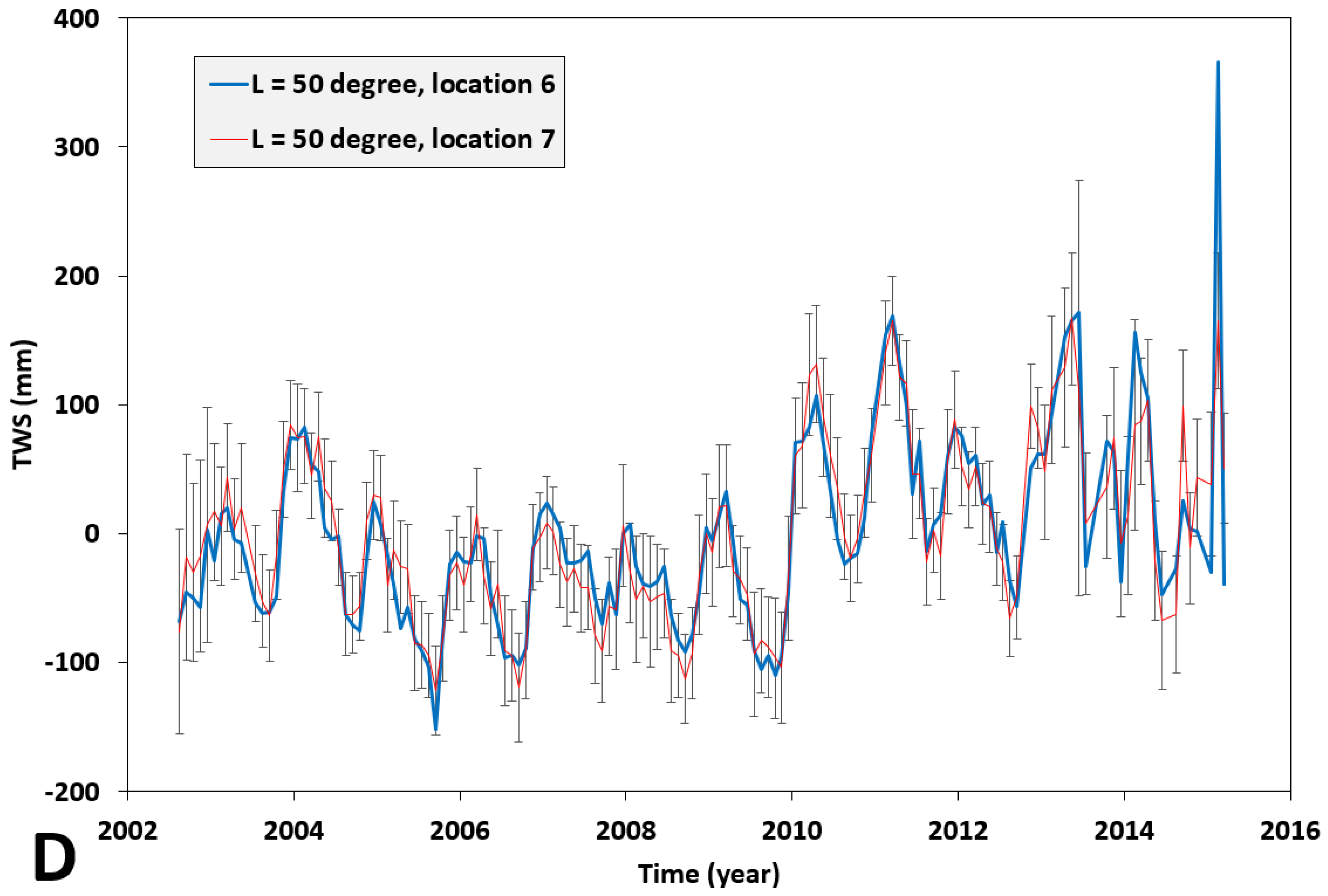
Figure 1. Relationship between rainfall and terrestrial water storage (TWS). TWS comprises surface water storage (SWS) in the surface zone, soil moisture storage (SMS) in the soil zone (SZ) and groundwater storage (GWS) in the saturated groundwater zone (SGZ). Water storage in the vadose zone (VZ) is considered to be in transit from the SMS to the GWS. P is precipitation, R is runoff, I is infiltration, ET is evapotranspiration, SWE is snow water equivalent, D is water in dams and Gd is groundwater discharge. (A): Following rainfall events, TWS increases as the result of changes in SWS, SMS, GWS and the water in transit across the VZ. Changes in GWS by recharge from rainfall are delayed by the transit through the VZ. (B): In the dry season, the TWS decreases because there is a decrease in SWS, SMS and GWS. In (A,B), grey color represents the soil zone (SZ), green color represents the vadose zone (VZ) and blue color represents the saturated zone (SGZ).
Hydrology 10 00187 g001aHydrology 10 00187 g001b
Figure 2. Geographical location of the study area in Andalucía, Southern Spain. The small purple dots are the centres of a regular grid of square cells with side lengths of 5 km. The large purple dots are eight locations at which the gravity-derived TWS time series are calculated. The red square is a 200 km × 200 km square centred at point 7. The dashed blue square represents a 400 km × 400 km square centred at point 7. The dashed green square represents a 400 km × 400 km square centred at point 6.
Hydrology 10 00187 g002
Figure 3. (A): Terrestrial water storage (TWS) for the 144 months between 2002 and 2015 for location 7 and maximum degrees for the spherical harmonics of L = 30 and L = 50. There is an evident annual cycle superimposed on the other cycles of longer periods. The high-frequency variations increase from a maximum degree of L = 30 to L = 50. (B): Terrestrial water storages (TWSs) for the same maximum degree L = 50 for two different locations 6 and 7. Note that the point location is a reference at which the support of the measurement is centred. The values are averages of squares of around 400 km side length for maximum degree L = 50 and 680 km for maximum degree L = 30. (C): Time series of the uncertainties of the TWS time series for location 7 and where the uncertainty was evaluated by the standard error (SE) or square root of the variance of the error described by Equation (2). (D): Time series of TWS for locations 6 and 7 (as in (B)) but where the TWS ±   SE is shown for location 7. The TWS for location 6 is within the TWS ±   SE of location 7 and thus both time series of locations 6 and 7 are indistinguishable if the uncertainties are considered.
Hydrology 10 00187 g003aHydrology 10 00187 g003bHydrology 10 00187 g003c
Figure 4. (A). Mean areal monthly rainfall around location 7 using a window of 200 km × 200 km and total rainfall for the entire Andalucía region. (B). Comparison of the mean rainfall for the 200 km × 200 km (red rectangle in Figure 2) and the TWS (mm) derived from the GRACE data using maximum degree L = 50.
Hydrology 10 00187 g004aHydrology 10 00187 g004b
Figure 5. Variation in the TWS using GRACE data for maximum degree L = 50 together with variation in mean temperature. The maximum temperature in summer corresponds to the minimum TWS, whereas the minimum temperature in winter corresponds to the maximum TWS due to the rainy season occurring in winter and spring.
Hydrology 10 00187 g005
Figure 6. (A). Periodogram for rainfall and TWS calculated from GRACE data for maximum degrees L = 30 (blue solid line) and L = 50 (red solid line). The main periodicities represent the yearly hydrologic cycle with a bimodal wet season and the climatic cycles. (B). Squared coherence spectrum between rainfall and TWS calculated from GRACE data for maximum degrees L = 50. (C). Achieved confidence level (%) of the squared coherence. (D). Phase spectrum (degree) between rainfall and TWS calculated from GRACE data for maximum degrees L = 50.
Hydrology 10 00187 g006aHydrology 10 00187 g006bHydrology 10 00187 g006c
Figure 7. Accumulated differences from the mean for rainfall (blue line) and TWS data (black line) for location 7, exhibiting three significant trends in the time series (red arrows). The first increases from the start of the time series at (a) to the maximum at (b). The second decreases from (b) to the minimum at (c). The third is from (c) to the end of the time series at (e). (d) is a significant inflexion in rainfall that does not appear as strongly in the TWS accumulated time series; the variability in TWS is less than that of rainfall because rainfall includes TWS and the water that was lost by runoff and evapotranspiration.
Hydrology 10 00187 g007
Figure 8. The 189 polygons (shaded grey) are the Andalucía groundwater bodies, each comprising one or more aquifers and, in total, comprising 62% of the total surface of the region. Between the groundwater bodies there are large zones with low-permeability lithologies (e.g., flysch, detritic mélange, metamorphic rocks) that are not proper aquifers but aquicludes and aquitards. The figure shows the spatial complexity of the distribution, which makes detailed monitoring of groundwater levels very difficult. In addition, most of the aquifers are subjected to pumping for irrigation and potable water and only a small number of piezometers can be regarded as being unaffected and measuring the real evolution of water levels. An expert selection of 11 representative piezometers (black dots) were used in this study; they are irregularly distributed and monitor only a small number of groundwater bodies.
Hydrology 10 00187 g008
Figure 9. Time series of the water head evolution for four of the piezometers shown in Figure 8 for the purpose of illustrating the complex nature of the groundwater level evolution in different aquifers.
Hydrology 10 00187 g009
Figure 10. Mean groundwater head anomaly calculated as the average of the groundwater head anomaly of the 11 piezometers shown in Figure 11. This is our best estimate of the evolution of GWS in Andalucía. First, all anomalies for each piezometer were calculated with respect to each mean and these were then averaged. Next, the anomalies were referred to the mean of the 2004–2009 period that is covered by the GRACE data.
Hydrology 10 00187 g010
Figure 11. Accumulated differences from the mean for rainfall (orange line), TWS data (black line) for location 7 and groundwater (blue line), for anomalies with respect to the mean for the period 2004–2009. The groundwater curve shows the general trends described in Figure 7, with a decrease (depletion) over a five-year period and a partial recovery in the following six years.
Hydrology 10 00187 g011
Figure 12. (A) TWS (GRACE maximum degree L = 30) time series and groundwater head anomalies in which there is a good correspondence between both signals over the annual cycle and the multi-year trends. (B) Time series of the rainfall and groundwater head anomalies in which there is a deficit of rain (drought) and a negative anomaly of the groundwater head that may imply depletion of groundwater resources. (C) TWS (GRACE maximum degree L = 30) time series and rainfall anomalies in which there is a good correspondence between both signals but with higher variability in rainfall. The very large spikes in rainfall do not correspond to the acute spikes in TWS because there is a proportional loss of water mass by runoff.
Hydrology 10 00187 g012aHydrology 10 00187 g012b
Figure 13. Time series of trends for the TWS (GRACE maximum degree L = 30) and groundwater head anomalies. A moving average filter, with a half-bandwidth of 12 months, was used. The trend shows similar behaviour between TWS and GWS but with a delay in the groundwater signal.
Hydrology 10 00187 g013
Table 1. Geographical co-ordinates of the 8 purple points represented in Figure 2.
PointLongitude (Degree)Latitude (Degree)
1−5.00436.745
2−2.76336.701
3−7.27838.543
4−4.97838.545
5−2.67838.501
6−6.12337.651
7−3.84537.628
8−1.58837.562
Disclaimer/Publisher’s Note: The statements, opinions and data contained in all publications are solely those of the individual author(s) and contributor(s) and not of MDPI and/or the editor(s). MDPI and/or the editor(s) disclaim responsibility for any injury to people or property resulting from any ideas, methods, instructions or products referred to in the content.

