Machine Learning-Based Predictions for Half-Heusler Phases

Abstract

Machine learning models (Support Vector Regression) were applied for predictions of several targets for 18-electron half-Heusler phases: a lattice parameter, a bulk modulus, a band gap, and a lattice thermal conductivity. The training subset, which consisted of 47 stable phases, was studied with the use of Density Functional Theory calculations with two Exchange-Correlation Functionals employed (GGA, MBJGGA). The predictors for machine learning models were defined among the basic properties of the elements. The most optimal combinations of predictors for each target were proposed and discussed. Root Mean Squared Errors obtained for the best combinations of predictors for the particular targets are as follows: 0.1 Å (lattice parameters), 11–12 GPa (bulk modulus), 0.22 eV (band gaps, GGA and MBJGGA), and 9–9.5 W/mK (lattice thermal conductivity). The final results of the predictions for a large set of 74 semiconducting half-Heusler compounds were disclosed and compared to the available literature and experimental data. The findings presented in this work encourage further studies with the use of combined machine learning and ab initio calculations.

1. Introduction

Half-Heusler (hH) phases continue to draw unwavering interest due to various possible applications, e.g., in optoelectronics [1,2], thermoelectric devices [1,3,4], and ferromagnets [5]. The stable hH compounds are limited to the 18 valence electron systems, i.e., ternary phases with stoichiometry of 1:1:1, XYZ (space group no $F\overline{4}3m$), where Z is a main group element, while X and Y are transition metals. Electronegativity determines the order of elements (Z is an anion) and their distribution in a unit cell, with Wyckoff positions X(1/4, 1/4, 1/4), Y(0, 0, 0), and Z(1/2, 1/2, 1/2).

Machine learning (ML) methods are nowadays widely used for cost-effective predictions of various parameters for half-Heusler (hH) phases, e.g., stability [6], atomic site preferences [7], band structures [8], lattice parameters [9], band gaps [10], lattice thermal conductivity [11,12,13], and spin polarization [14]. Furthermore, the lattice thermal conductivity was investigated for the double hH alloys [15], which exhibit relatively larger and more complex unit cells than those in hH materials. Such findings highly encourage further investigations of the possible ML support for ab initio methods and assure that the elemental properties can be successfully used for the predictions of structural and electronic properties of various intermetallics. Moreover, the ML approach is highly efficient when compared to the high-throughput DFT calculations. The ab initio studies may be very resource-consuming, due to the use of advanced Exchange-Correlation Functionals (XCF) such as hybrid functionals with an exact-exchange term. Expanding the database of potentially valuable hH systems may be accelerated thanks to a reasonable set of previously studied materials (training subset); further investigations may be optimized and supported via ML methods. It was already revealed that elemental features of ions may be sufficient input for predictions of various properties of hH alloys. Predictors proposed by Miyazaki et al. [12] were atomic mass and radius, density of a solid, molar volume, and Debye temperature. Additionally, Zhang et al. [9] considered electronegativity as a key predictor for modeling of lattice parameters.

In this work, several targets for a large set of stable hH alloys are investigated: lattice parameter a, bulk modulus B, band gap $E_{XCF}$ (where $XCF=GGA,MBJ$), and lattice thermal conductivity ${\kappa }_L$. These properties for the training subset are also explicitly calculated by employing the Density Functional Theory (DFT), and the results of the ML predictions and DFT calculations are compared. The ML approach used is Support Vector Regression (SVR) with Gaussian Radial Basis Function. Numerous sets of feature spaces are considered with the Valence Electron Count (VEC) and the first, second, and third ionization energies included. The selection of predictors is carefully studied and discussed. A satisfactory accordance between the predicted and available theoretical and experimental data for various hH phases is found. Furthermore, numerous novel materials are considered and characterized.

2. Computational Details

Compounds investigated in this paper were limited by the valence electron count of 18, which is crucial for stability of hH alloys [16]. DFT calculations were performed with the use of VASP [17,18,19,20] with spin–orbit coupling included. The cut-off energy of the plane–wave basis was set to 500 eV, and the XCF parameterizations employed were Generalized Gradient Approximation (GGA) [21] and modified Becke–Johnson GGA (MBJGGA) [22]. Lattice thermal conductivity ${\kappa }_L$ was calculated following Slack’s equation [23,24,25].

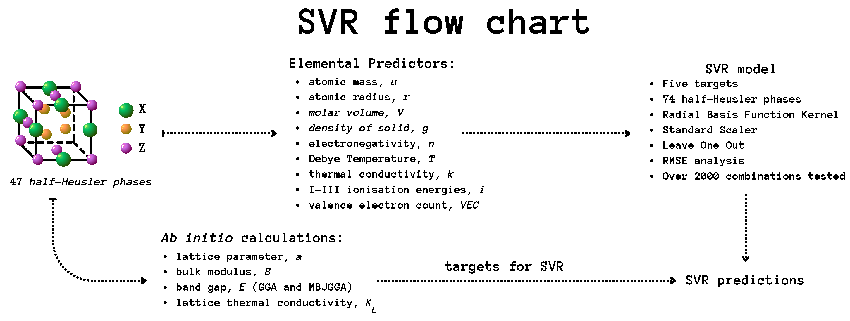
The general idea behind ML is to solve the regression issue and, therefore, to find a function that provides mapping from an input to a training sample target. Methods of solving the regression problem are numerous, based on the different mathematical models, e.g., Random Forest Regression [11], Multiple Linear Regression, and Boosted Decision Tree Regression [12]. SVR models perform the hyperplane analysis in the feature space, which maximizes the number of points that are inside the decision boundary line [26]. Different types of kernel functions enable the best model fit, depending on the data provided [27]. SVR was already shown to be successful in similar applications [28]. The methodology used in this work is depicted in Figure 1.

The elemental features for predictor sets were taken from the WebElements periodic table (University of Sheffield [29]). SVR methods implemented in sklearn library [30] with Gaussian Radial Basis Function [31] were used. SVR parameters, i.e., C and $\gamma$ (responsible for the trade-off between regularization and fitting the training data and for the flexibility of the model), were determined as one and $1/(n\ast X_{VAR})$, where n is the number of features and $X_{VAR}$ is a variation in the predictors subset. The feature scaling (Standard Scaler) was applied. The cross-validation of models tested was the Leave One Out (LOO) approach [32]. The quantitative accuracy of SVR models was determined by Root Mean Squared Error (RMSE) defined as $\sqrt{\frac{1}{n}{\sum }_{i=1}^n{(a_i^{calc}-a_i^{pred})}^2}$, where a is a studied quantity.

3. Results

The training subset of 47 18-valence electron hH phases considered in this work consists of 32 stable compounds (according to the Open Quantum Materials Database, OQMD [33]), as reported in the literature [34], and 15 systems with hull distance less or equal to 0.1 eV, which in many cases indicates stable phases (Aykol et al. [35]). The 32 stable compounds were already comprehensively investigated as candidates for thermoelectric materials [4]. The structural and electronic properties of 15 additional phases are gathered in

Table 1. The 18-valence electron hH systems with hull distance: 0 eV < $E_{HD}$ ≤ 0.1 eV [33,35]. Structural and electronic parameters: lattice parameter a (Å), bulk modulus B (GPa), band gap with GGA parameterization $E_{GGA}$ (eV), band gap with MBJGGA parameterization $E_{MBJ}$ (eV), lattice thermal conductivity ${\kappa }_L$ (W/mK).

Comp.	a	B	${\mathit{E}}_{\mathit{GGA}}$	${\mathit{E}}_{\mathit{MBJ}}$	${\mathit{\kappa }}_{\mathit{L}}$
TiPdPb	6.328	103.88	0.352	0.324	55.57
TiPdGe	5.964	131.38	0.619	0.584	45.00
VRhGe	5.796	172.54	0.433	0.748	38.73
ZrCoAs	5.831	147.58	1.203	1.228	68.47
ZrRhAs	6.110	143.97	1.117	1.292	59.94
HfPdGe	6.142	133.71	0.552	0.506	66.63
HfRhAs	6.063	160.02	0.282	0.816	58.39
TaRhGe	5.973	185.13	1.044	1.026	64.25
VRuSb	6.044	165.64	0.189	0.631	42.96
ZrNiGe	5.893	141.57	0.679	0.654	74.56
ScPdAs	6.098	111.31	0.432	0.451	42.58
NbRuAs	5.961	183.13	0.337	0.506	53.07
TiNiPb	6.038	115.66	0.341	0.292	66.00
NbRuBi	6.307	151.77	0.383	0.557	57.56
LuNiAs	5.989	106.94	0.408	0.475	65.65

. It is crucial to note that the further training of ML models is based on systems that are expected to be stable and feasible to be synthesized.

Some properties of the systems presented in Table 1 were already investigated in the literature, e.g., the cubic lattice parameters (a) of 5.964 and 6.327 Å were theoretically calculated for TiPdGe and TiPdPd, respectively [36]. The reported values of the bulk modulus (B) were 132.41 and 104.14 GPa, while band gaps ($E_g$) were 0.66 and 0.386 eV (PBE-GGA), for the Ge- and Pb-bearing systems. The results presented in this work for TiPdGe and TiPdPb are very similar to the literature data. Furthermore, the GGA predictions were also reported for VRhGe [37], indicating a of 5.73 Å, B of 186.1 GPa, and $E_g$ of 0.34 eV. While the lattice parameter calculated here is almost the same, the bulk modulus and band gap are slightly different from the literature data. The discrepancy may be caused by the different XCF and DFT implementations used. Bendahma et al. [38] predicted a for HfPdGe of 11.62 Bohr, B of 137.33 GPa, and $E_g$ of 0.55 eV, which are very close to the results obtained here. Interestingly, TaRhGe was experimentally synthesized in the TiNiSi-type hexagonal structure [39]. Theoretical studies of lattice parameters, bulk modulus, GGA, and MBJGGA band gaps for VRuSb led to the following values: 5.940 Å, 190.35 GPa, 0.22 eV, and 0.64 eV, respectively [40,41]. The arsenide ScPdAs was predicted as a phase with a of 6.14 Å, B of 106.90 GPa, and $E_g$ of 0.44 eV [42]. The value of ${\kappa }_L$ (35 W/mK at 300 K) calculated according to the modified Debye–Callaway model is very close to the results obtained for this system via Slack’s formula. Nearly the same ${\kappa }_L$ was also obtained for LuNiAs, which is clearly lower than the one presented in this work, although other properties obtained for this system are in good accordance. Calculations for TiNiPb presented by Hong et al. [43] revealed an a value which differs by 0.1 Å. The value of ${\kappa }_L$ for ZrCoAs was estimated by Carrete et al. [11] to be 24.0 W/mK, whereas, for NiPbTi, it was 109 W/mK. Similar values of ${\kappa }_L$ were obtained for BBeGa and BMgGa by Sun et al. with the Slack-derived methodology [24].

The number of hH materials gathered in Table 1 is limited by the assumption about the acceptable hull distance for stable phases [35]. One should also perceive the training subset as versatile enough to prepare the feature space related to compounds with different values of the targets desired, as pointed out by Tranås et al. [13]. For the training subset, the lattice parameters range from 5.496 (VFeAs) to 6.525 Å (ScPdBi), the bulk moduli range from 85.35 (ScPdBi) to 203.24 GPa (VIrGe), the GGA band gaps range from 0.071 (ScPdBi) to 1.300 eV (TiCoAs), the MBJGGA band gaps range from 0.121 (ScPdBi) to 1.361 eV (HfCoAs), and the lattice thermal conductivities range from 38.73 (VRhGe) to 113.52 W/mK (HfNiSn). Such wide ranges of structural and electronic properties indicate that multiple diverse ternary systems with various parameters were used for the model training. Finally, the various ions present in the training subset enable wide and reliable predictions for numerous ternary systems.

The feature space (Figure 1) used for the description of the hH systems consisted of the following elemental properties [29]:

• Atomic mass, u;
• Atomic radius, r;
• Molar volume, V;
• Density of solid, g;
• Electronegativity, n;
• Debye temperature, T;
• Thermal conductivity, k;
• I–III ionization energies, i(I), i(II), i(III);
• Valence Electron Count, VEC.

The parameters listed above were regarded for all ions with all atomic sites, i.e., denoting that parameter $\alpha$ was included in the feature space means that ${\alpha }_X$, ${\alpha }_Y$, and ${\alpha }_Z$ were included. This approach, well described by Miyazaki et al. [12], provides comprehensive insight about the distribution of the particular property in the whole set of ternary systems investigated.

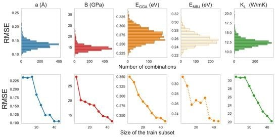
The convergence of the SVR models as a function of the size of the training subset was determined based on RMSE, as presented in Figure 2 (learning curves with targets split into subplots (a) and (b) due to the order of magnitude). For lattice parameters and band gaps with both XCF regarded, one can note a clear decrease in RMSE and all 3 curves reach a plateau at the point of 40 records in the training set. Therefore, there may be no need to acquire more input data calculations for the training since the performance of the model may not significantly improve. RMSE for a, $E_{GGA}$, and $E_{MBJ}$ improved from 0.235 to 0.105 Å, from 0.350 to 0.235 eV, and from 0.314 to 0.225 eV, respectively.

As depicted in Figure 2b, no clear plateau is observed in learning curves for B and ${\kappa }_L$. However, the value of RMSE obtained for B is already relatively low. Although a further extension of the training set is expected to decrease RMSE of ${\kappa }_L$, one may also consider that an arbitrary selection of the predictor set for this quantity is less favorable than in the cases of simple structural properties such as a or B. The decreases in RMSE between the minimal and 47 compound training sets are about 15 GPa for bulk modulus and 11 W/mK for lattice thermal conductivity. The final values of RMSE for B and ${\kappa }_L$ are about 13 GPa and 20 W/mK, respectively, which seems to be a good accuracy, according to the order of magnitude of these parameters. The training set of 47 hH alloys is, therefore, large enough to derive reliable and repeatable results for further predictions.

Contrary to the five-fold cross-validation used by Miyazaki et al. [12], the Leave One Out (LOO) cross-validation approach was used in this work. This choice was motivated by the LOO efficiency within the Support Vector Machine family [44,45]. In this method, only one record among the whole feature space set is determined as the value to be predicted and compared with the actual result. Iteration of such a method over all the records in the feature space enables achieving a constant RMSE among the models for a particular set of predictors. Depending on the combinations of predictors used, RMSE may further vary. In general, one may expect that a lower RMSE would characterize a better model. However, in fact, low RMSE does not unequivocally determine the best combination of predictors. The particular subset of parameters in each combination of the elemental features may yield better predictions for some phases and worse results for others. The fact that RMSE is an average is worth considering in many cases.

Numerous ML band gap predictions for organic [46] and inorganic solids [28,47], MXenes [48], perovskites [49], and other systems [50,51,52] were carefully discussed in the literature. However, there are still few reports on band gap predictions for hH phases [10]. Olsthoorn et al. [46] obtained the lowest RMSE of 0.519 eV, whereas the results of Lee et al. [28] exhibited RMSE of 0.24 eV. Finally, Choudhary et al. [10] disclosed RMSE of 0.286 eV, which is also larger than the RMSE obtained in our research (about 0.22 eV).

For each target, over 2000 combinations of the elemental predictors were tested, from 1-element feature spaces (e.g., atomic radii of XYZ ions: $r_X,r_Y,r_Z$) to the most complex feature space consisting of 11 predictors for each ion in the particular phase. The summaries of RMSE as a function of the number of elemental predictors are depicted in Figure 3. As one may expect, the discrepancy between the ML- and DFT-derived results is maximal for one predictor feature spaces due to oversimplification. While the extension of the predictor set generally improves the model performance, the best sets are based on 3–4 elemental features, which are characteristic of particular targets. This effect is related to the fact that bigger predictor sets include many features that may be unsuitable for SVR in each case.

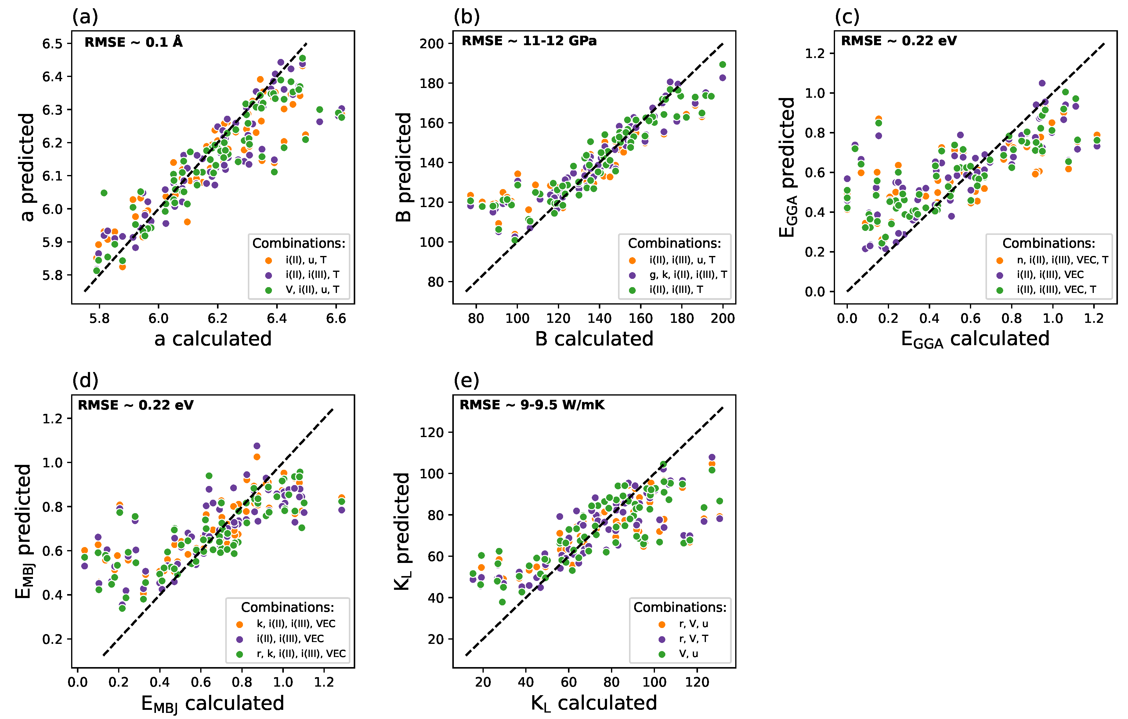
The scatter plots (ML-predicted vs. DFT-calculated) for three favorable combinations of predictors are depicted for all targets in Figure 4. The Debye temperature and thermal conductivity occurred most often in the best RMSE combinations for the target of lattice parameter. An analysis of three combinations of predictors with the lowest and comparable RMSE of 0.1 Å provides different distributions of the predictions among the 47 systems, as presented in Figure 3a. The RMSE values among the predictor sets selected here are very close to each other. The four-predictor set [V, i(II), u, T] seems to be the best approach for the majority of compounds in the training set. However, in some cases, e.g., for VIrGe (a${}_{calc}$ = 5.818 Å), this set leads to a worse prediction when compared to those of [i(II), i(III), T] and [i(II), u, T]. The selection of the best predictor set is, therefore, a challenging task, which requires a careful analysis of the data presented in scatter plots.

The best models for bulk modulus are strongly connected with the third ionization energy. The predictor set with the lowest RMSE for bulk modulus (Figure 4b) is [i(II), i(III), T]. Merging the additional predictors to this feature space resulted in a slight increase in RMSE (0.32 GPa for additional [g, k] and 0.42 GPa for additional [u]). Enriched feature spaces neither provide better single predictions for the boundary cases nor yield lower RMSE.

For $E_{GGA}$ (Figure 4c) and $E_{MBJ}$ (Figure 4d), the second and third ionization energies of the constituent elements are present in sets with the lowest RMSE. The model based on [i(II), i(III), VEC, T] seems to perform slightly better than the other ones. Reasonable results for $E_{GGA}$ require VEC, which illustrates the importance of optimum distribution of the valence electrons in the hH alloys for insights into electronic structure of such systems. Similar findings are revealed for the best combinations of predictors for $E_{MBJ}$ (Figure 4d). In addition to the ionization energies, VEC, thermal conductivity, and ionic radius are favorable as the third predictor.

In the case of the lattice thermal conductivity (Figure 4e), the volume and atomic mass were regarded as the best predictors for SVR models. Combining or replacing them with the atomic radius or Debye temperature leads to higher RMSE. Models for this quantity do not require any of [i(II), i(III)], a fact which is related to Slack’s formula.

After analyses of the best predictor sets, the favorable ones for particular targets are as follows:

• a: [V, i(II), u, T];
• B: [i(II), i(III), T];
• $E_{GGA}$: [i(II), i(III), VEC, T];
• $E_{MBJ}$: [r, k, i(II), i(III), VEC];
• ${\kappa }_L$: [V, u].

One shall notice that the most common parameters are the ionization energies. The significance of the second and third ionization energies for various targets may be useful for further ML modeling for similar intermetallics.

The overall performance of SVR models is limited not only by the size of the training set and variation of elements, but also by the characteristic features of materials that exhibit extremal values of targets. As depicted in Figure 4b, the error in predictions for relatively low values of bulk modulus reaches 40 GPa, which is high when compared with RMSE of 12 GPa. The electronic structures of hH systems with narrow or relatively wide band gaps are also difficult to predict with ML methods. Namely, band structures of bisimides and antimonides are unique, and many hH systems are on the edge of a transition between the very narrow $E_g$ and topological insulator. The training set of semiconducting materials could be extended with phases with zero or negative band gaps. This finding may be an interesting direction for further ML-based studies on $E_g$ in intermetallics. A similar issue is found for predictions of ${\kappa }_L$, i.e., the most interesting values of ${\kappa }_L$ for thermoelectrics are low. The materials with low ${\kappa }_L$ are rare and difficult to predict even based on relatively large training sets because the SVR models are dominated by average properties of materials.

The final SVR predictions for 74 hH phases, which were not studied here with the DFT-based calculations, are gathered in

Table 2. Predicted values of the lattice parameter a (Å), bulk modulus B (GPa), band gap with GGA parametrization $E_{GGA}$ (eV), band gap with MBJGGA parametrization $E_{MBJ}$ (eV), and lattice thermal conductivity ${\kappa }_L$ (W/mK).

Comp.	a	B	E${}_{\mathit{GGA}}$	E${}_{\mathit{MBJ}}$	K${}_{\mathit{L}}$	Comp.	a	B	E${}_{\mathit{GGA}}$	E${}_{\mathit{MBJ}}$	K${}_{\mathit{L}}$
HfNiGe	5.893	151.53	0.74	0.70	79.52	TiNiSn	5.918	124.13	0.43	0.49	62.46
HfRhBi	6.331	128.63	0.64	0.76	86.65	TiPdSn	6.20	114.38	0.43	0.46	57.02
HfNiPb	6.175	129.51	0.46	0.48	94.83	TiPtPb	6.342	128.13	0.57	0.60	72.91
HfRhSb	6.284	138.78	0.65	0.78	104.5	TiCoSb	5.843	135.62	0.92	0.92	61.96
HfPdPb	6.353	124.08	0.39	0.39	92.69	TiRhSb	6.110	135.24	0.66	0.83	59.22
HfPtSn	6.348	143.19	0.69	0.82	95.28	TiIrAs	5.952	171.78	0.72	0.94	51.43
HfPtPb	6.369	138.14	0.62	0.70	92.82	TiIrBi	6.258	144.95	0.63	0.82	67.39
HfCoSb	6.028	134.71	0.97	0.96	101.62	VCoSn	5.813	150.09	0.57	0.82	50.27
LuNiSb	6.142	118.59	0.45	0.53	86.67	VRhSn	6.018	152.80	0.41	0.68	42.65
LuPdSb	6.300	118.32	0.39	0.42	90.92	VIrSn	6.052	171.75	0.38	0.65	55.34
LuNiBi	6.185	117.78	0.47	0.57	83.54	VRuAs	5.844	176.39	0.24	0.73	37.81
NbRhGe	5.942	176.72	0.78	0.88	53.10	VOsSb	6.051	163.10	0.32	0.60	59.10
NbOsAs	5.992	173.71	0.42	0.59	57.95	VRuBi	6.183	154.00	0.27	0.63	46.24
NbOsBi	6.319	153.33	0.46	0.53	73.17	VOsAs	5.854	173.33	0.32	0.65	44.98
NbRhSn	6.195	152.96	0.62	0.78	70.38	VOsBi	6.200	155.11	0.36	0.60	60.37
NbRhPb	6.317	142.94	0.58	0.67	67.46	VCoPb	6.004	142.22	0.53	0.62	56.36
NbIrPb	6.317	162.40	0.58	0.64	79.63	VRhPb	6.175	143.60	0.40	0.59	47.93
NbCoSn	5.940	150.13	0.81	0.92	74.59	VIrPb	6.192	161.41	0.41	0.61	62.40
NbCoPb	6.104	141.06	0.73	0.73	73.26	VFeBi	6.052	150.48	0.41	0.64	51.61
NbOsSb	6.228	162.70	0.43	0.52	83.18	YNiAs	6.058	124.92	0.53	0.54	58.54
NbFeSb	5.932	160.15	0.62	0.74	74.12	YNiSb	6.157	121.03	0.49	0.55	66.32
NbFeBi	6.144	145.50	0.62	0.70	66.30	YNiBi	6.209	120.66	0.48	0.57	67.77
ScNiAs	6.048	126.16	0.71	0.69	58.06	YPdAs	6.111	121.33	0.42	0.49	49.56
ScNiSb	6.172	111.29	0.60	0.59	66.83	YPdSb	6.290	118.01	0.35	0.45	65.94
ScNiBi	6.239	106.29	0.56	0.58	68.60	YPtSb	6.276	128.57	0.51	0.59	69.09
ScPdSb	6.348	100.79	0.34	0.34	66.58	ZrNiSn	6.072	123.54	0.48	0.52	85.14
ScPtSb	6.333	120.26	0.58	0.64	69.62	ZrNiPb	6.177	119.30	0.42	0.46	82.71
TaRhSn	6.131	162.94	0.82	0.89	87.23	ZrPdGe	6.149	130.13	0.63	0.55	62.95
TaRhPb	6.206	155.14	0.75	0.76	84.45	ZrPdPb	6.455	110.42	0.39	0.38	82.90
TaIrGe	6.015	189.33	0.80	0.85	69.30	ZrPtSn	6.389	130.93	0.71	0.84	89.55
TaIrSn	6.159	172.9	0.75	0.79	89.15	ZrCoSb	6.014	127.17	1.00	0.93	87.32
TaIrPb	6.212	164.16	0.71	0.70	86.42	ZrCoBi	6.155	119.47	0.91	0.84	78.01
TaRuSb	6.108	173.42	0.46	0.64	93.97	ZrRhSb	6.307	126.79	0.76	0.82	92.14
TaRuBi	6.195	161.39	0.49	0.61	79.00	ZrRhBi	6.384	118.40	0.71	0.77	74.73
TaOsSb	6.165	164.87	0.51	0.59	94.12	ZrIrAs	6.110	160.96	0.85	0.94	66.41
TaCoPb	6.086	153.94	0.89	0.82	88.35	ZrIrSb	6.304	147.57	0.76	0.82	96.04
TaFeBi	6.110	156.66	0.76	0.78	84.33	ZrIrBi	6.360	138.67	0.72	0.77	83.56

. The structural and electronic properties of some alloys among this set were already investigated in the literature. Adetunji et al. [53] reported some properties of the cubic HfNiGe phase, i.e., a of 5.861 Å, B of 143.1 GPa, and $E_g$ of 0.61 eV. These three values are very close to our predictions and are consistent with the RMSE of the related SVR models. Interestingly, the value of $E_g$ obtained here for NbRhGe is strongly underestimated when compared to the literature data [54], in spite of the fact that several novel germanides were included in the training set.

The electronic structure of ScNiAs was investigated by Jaishi et al. [55], revealing a of 5.84 Å and $E_g$ values of 0.48 (GGA) and 0.52 eV (MBJGGA). The lattice parameter predicted here is larger by 0.2 Å than the DFT result, whereas the $E_g$ values are close to the literature data. One may connect this fact with the presence of numerous arsenides present in our training set.

Previous theoretical investigations for HfRhBi revealed a, B, and $E_g$ of 6.41 Å, 127.62 GPa, and 0.17 eV, respectively [56]. The thermal conductivity of HfRhBi was reported as up to 40 W/mK at 300 K (significantly smaller than our predictions). Kangsabanik et al. [56] also reported similar results for ZrIrBi and ZrRhBi, disclosing ${\kappa }_L$ (W/mK) of up to 55 and 30 W/mK, respectively. The discrepancy between our predictions and the literature data for ${\kappa }_L$ is caused mainly by the methodology used for calculations (Slack’s formula vs. phonon spectra, etc.). There is also a significant discrepancy between the band gaps, i.e., predicted 0.71 eV versus calculated 0.26 eV and predicted 0.77 eV versus calculated 1.02 eV for ZrIrBi and ZrRhBi, respectively. One may explain this issue by considering that the band structures of these materials, the fact that the number of bisimides in our training set is limited, and the performance of our SVR approach is poor for narrow band gap materials. The reported a for TiIrBi ranged from 6.309 to 6.358 Å, depending on the alloy model [57], which is in good accordance with the value predicted here. The range of reported B was from 104.4 up to 123.7 GPa, which is slightly lower than our result. However, the GGA- and MBJGGA-derived band gaps (0.56 and 0.87 eV, respectively) are in very good accordance with the predictions presented here.

The analysis for ScMSb (M = Ni, Pd, and Pt) indicates very good accordance between the DFT-derived a and B and the SVR [58]. However, the SVR-predicted values of a for LuPdSb, YNiSb, and YPdSb differ from the calculated ones by 0.2–0.3 Å, which are clearly higher values than the RMSE of the model. Furthermore, the predicted band gaps for antimonides, ScMSb and (Lu;Y)(Ni;Pd)Sb, are strongly overestimated when compared with the calculated ones. This effect is connected with the characteristic features of electronic structures of hH antimonides and bisimides [58,59,60,61,62]. Bands at Valence Band Maximum (VBM) in these systems exhibit very small effective mass, which is not present in systems in our training set. Amont the hH antimonides, NbFeSb is the most studied material. The experimental lattice parameter value (5.949 Å [63]) and the calculated value (5.968 Å [64]) are in very good accordance with our predictions. The $E_g$ of 0.51 eV is also close to the predicted value of 0.62 eV, whereas the reported values of ${\kappa }_L$ are lower than that predicted here.

The SVR predictions for NbCoSn are in good agreement with the reported data [65]. The lattice thermal conductivity of CoSbZr was calculated by Carrete et al. [11] to be 25 W/mK, while ${\kappa }_L$ of 109 W/mK was calculated for FeNbP and NiPbTi. Furthermore, the calculated ${\kappa }_L$ for RuAsV (23.5 W/mK) with the declared standard deviation of 13% is in good accordance with our predicted value for VRuAs (37.81 W/mK).

4. Conclusions

In summary, all SVR models considered in this work lead to very good predictions for lattice parameters and bulk modulus. The ML-derived values of band gaps and lattice thermal conductivity may be strongly affected by specific electronic structures among the phases regarded, e.g., the direct–indirect type of the band gap and the spectrum of carrier concentration. The significance of the second and third ionization energies of the elements in the process of predicting different targets of complex alloys, i.e., lattice parameter, bulk modulus, and band gap (GGA and MBJGGA), is an important insight into the selection of feature spaces for ML support of the ab initio calculations. The predictions obtained here for 74 hH alloys are in good accordance with the available literature data, especially for the well-known NbFeSb compound, which indicates good predictive power of SVR models.

References

- Dubey, S.; Abraham, J.A.; Dubey, K.; Sahu, V.; Modi, A.; Pagare, G.; Gaur, N.K. DFT study of RhTiP half Heusler semiconductors: Revealing its mechanical, optoelectronic, and thermoelectric properties. Phys. B Condens. Matter 2024, 672, 415452. [Google Scholar] [CrossRef]
- Azzi, S.; Belkharroubi, F.; Ramdani, N.; Messaoud, I.S.; Belkilali, W.; Drici, L.; Blaha, L.; Ameri, I.; Al-Douri, Y.; Bouhemadou, A. Investigation of optoelectronic properties of half-Heusler KZnN and KZnP compounds. Rev. Mex. Fis. 2023, 69, 060501-1. [Google Scholar] [CrossRef]
- Sartipi, E.; Elahi, S.M.; Hantehzadeh, M.R.; Boochani, A.; Ghoranneviss, M. Giant magneto-optical Kerr effect and thermoelectric properties in CeBiPt half-Heusler by DFT. Mod. Phys. Lett. B 2023, 2350253. [Google Scholar] [CrossRef]
- Bilińska, K.; Winiarski, M.J. High-Throughput Exploration of Half-Heusler Phases for Thermoelectric Applications. Crystals 2023, 13, 1378. [Google Scholar] [CrossRef]
- Sudharsan, J.B.; Srinivasan, M.; Elavarasan, N.; Ramasamy, P.; Fujiwara, K. Ferrimagnetic half Heusler alloys for waste heat recovery application-First principle study using different exchange–correlation functionals. J. Magn. Magn. Mater. 2023, 588, 171409. [Google Scholar]
- Legrain, F.; Carrete, J.; van Roekeghem, A.; Madsen, G.K.; Mingo, N. Materials screening for the discovery of new half-Heuslers: Machine learning versus ab initio methods. J. Phys. Chem. B 2018, 122, 625–632. [Google Scholar] [CrossRef]
- Gzyl, A.S.; Oliynyk, A.O.; Adutwum, L.A.; Mar, A. Solving the Coloring Problem in Half-Heusler Structures: Machine-Learning Predictions and Experimental Validation. Inorg. Chem. 2019, 58, 9280–9289. [Google Scholar] [CrossRef]
- Dylla, M.T.; Dunn, A.; An, S.; Jain, A.; Snyder, G.J. Machine learning chemical guidelines for engineering electronic structures in half-heusler thermoelectric materials. Research 2020, 2020, 6375171. [Google Scholar] [CrossRef]
- Zhang, Y.; Xu, X. Machine learning modeling of lattice constants for half-Heusler alloys. AIP Adv. 2020, 10, 045121. [Google Scholar] [CrossRef]
- Choudhary, M.K.; Raj V, A.; Ravindran, P. Composition and Structure Based GGA Bandgap Prediction Using Machine Learning Approach. arXiv 2023, arXiv:2309.07424. [Google Scholar]
- Carrete, J.; Li, W.; Mingo, N.; Wang, S.; Curtarolo, S. Finding unprecedentedly low-thermal-conductivity half-Heusler semiconductors via high-throughput materials modeling. Phys. Rev. X 2014, 4, 011019. [Google Scholar] [CrossRef]
- Miyazaki, H.; Tamura, T.; Mikami, M.; Watanabe, K.; Ide, N.; Ozkendir, O.M.; Nishino, Y. Machine learning based prediction of lattice thermal conductivity for half-Heusler compounds using atomic information. Sci. Rep. 2021, 11, 13410. [Google Scholar] [CrossRef]
- Tranås, R.; Løvvik, O.M.; Tomic, O.; Berl, K. Lattice thermal conductivity of half-Heuslers with density functional theory and machine learning: Enhancing predictivity by active sampling with principal component analysis. Comput. Mater. Sci. 2022, 202, 110938. [Google Scholar] [CrossRef]
- Kurniawan, I.; Miura, Y.; Hono, K. Machine learning study of highly spin-polarized Heusler alloys at finite temperature. Phys. Rev. Mater. 2022, 6, L091402. [Google Scholar] [CrossRef]
- Filanovich, A.N.; Povzner, A.A.; Lukoyanov, A.V. Machine learning prediction of thermal and elastic properties of double half-Heusler alloys. Mater. Chem. Phys. 2023, 306, 128030. [Google Scholar] [CrossRef]
- Gautier, R.; Zhang, X.; Hu, L.; Yu, L.; Lin, Y.; Sunde, T.O.; Chon, D.; Paeppelmeirer, K.; Zunger, A. Prediction and accelerated laboratory discovery of previously unknown 18-electron ABX compounds. Nat. Chem. 2015, 7, 308–316. [Google Scholar] [CrossRef]
- Kresse, G.; Hafner, J. Ab initio molecular dynamics for open-shell transition metals. Phys. Rev. B 1993, 48, 13115. [Google Scholar] [CrossRef]
- Kresse, G.; Hafner, J. Ab initio molecular-dynamics simulation of the liquid-metal–amorphous-semiconductor transition in germanium. Phys. Rev. B 1994, 49, 14251. [Google Scholar] [CrossRef]
- Kresse, G.; Furthmüller, J. Efficiency of ab-initio total energy calculations for metals and semiconductors using a plane-wave basis set. Comput. Mater. Sci. 1996, 6, 15–50. [Google Scholar] [CrossRef]
- Kresse, G.; Furthmüller, J. Efficient iterative schemes for ab initio total-energy calculations using a plane-wave basis set. Phys. Rev. B 1996, 54, 11169. [Google Scholar] [CrossRef]
- Perdew, J.P.; Burke, K.; Ernzerhof, M. Generalized gradient approximation made simple. Phys. Rev. Lett. 1996, 77, 3865. [Google Scholar] [CrossRef]
- Tran, F.; Blaha, P. Accurate band gaps of semiconductors and insulators with a semilocal exchange-correlation potential. Phys. Rev. Lett. 2009, 102, 226401. [Google Scholar] [CrossRef]
- Slack, G.A. Nonmetallic crystals with high thermal conductivity. J. Phys. Chem. Solids 1973, 34, 321–335. [Google Scholar] [CrossRef]
- Sun, H.L.; Yang, C.L.; Wang, M.S.; Ma, X.G. Remarkably high thermoelectric efficiencies of the half-Heusler compounds BXGa (X = Be, Mg, and Ca). ACS Appl. Mater. Interfaces 2020, 12, 5838–5846. [Google Scholar] [CrossRef]
- Yang, K.; Wan, R.; Zhang, Z.; Lei, Y.; Tian, G. First-principle investigation on the thermoelectric and electronic properties of HfCoX (X = As, Sb, Bi) half-Heusler compounds. J. Solid State Chem. 2022, 312, 123386. [Google Scholar] [CrossRef]
- Awad, M.; Khanna, R.; Awad, M.; Khanna, R. Support vector regression. In Efficient Learning Machines: Theories, Concepts, and Applications for Engineers and System Designers; Springer: Berlin/Heidelberg, Germany, 2015; pp. 67–80. [Google Scholar]
- Rohmah, M.F.; Putra, I.K.G.D.; Hartati, R.S.; Ardiantoro, L. Comparison four kernels of svr to predict consumer price index. J. Phys. Conf. Ser. 2021, 1737, 012018. [Google Scholar] [CrossRef]
- Lee, J.; Seko, A.; Shitara, K.; Nakayama, K.; Tanaka, I. Prediction model of band gap for inorganic compounds by combination of density functional theory calculations and machine learning techniques. Phys. Rev. B 2016, 93, 115104. [Google Scholar] [CrossRef]
- WebElements. Available online: https://www.webelements.com (accessed on 13 November 2023).
- Pedregosa, F.; Varoquaux, G.; Gramfort, A.; Michel, V.; Thirion, B.; Grisel, O.; Blondel, M.; Prettenhofer, P.; Weiss, R.; Dubourg, V.V.; et al. Scikit-learn: Machine Learning in Python. J. Mach. Learn. Res. 2011, 12, 2825–2830. [Google Scholar]
- Fornberg, B.; Larsson, E.; Flyer, N. Stable computations with Gaussian radial basis functions. SIAM J. Sci. Comput. 2011, 33, 869–892. [Google Scholar] [CrossRef]
- Elisseeff, A.; Pontil, M. Leave-one-out error and stability of learning algorithms with applications. NATO Sci. Ser. III Comput. Syst. Sci. 2003, 190, 111–130. [Google Scholar]
- S Kirklin, S.; Saal, J.E.; Meredig, B.; Thompson, A.; Doak, J.W.; Aykol, M.; Rühl, S.; Wolverton, C. The Open Quantum Materials Database (OQMD): Assessing the accuracy of DFT formation energies. Npj Comput. Mater. 2015, 1, 15010. [Google Scholar] [CrossRef]
- Bilińska, K.; Winiarski, M.J. Search for semiconducting materials among 18-electron half-Heusler alloys. Solid State Commun. 2023, 365, 115133. [Google Scholar] [CrossRef]
- Aykol, M.; Dwaraknath, S.S.; Sun, W.; Persson, K.A. Thermodynamic limit for synthesis of metastable inorganic materials. Sci. Adv. 2018, 4, eaaq0148. [Google Scholar] [CrossRef]
- Kalita, D.; Limbu, N.; Ram, M.; Saxena, A. DFT study of structural, mechanical, thermodynamic, electronic, and thermoelectric properties of new PdTi Z (Z = Ge and Pb) half Heusler compounds. Int. J. Quantum Chem. 2022, 122, e26951. [Google Scholar] [CrossRef]
- Solola, G.T.; Bamgbose, M.K.; Adebambo, P.O.; Ayedun, F.; Adebayo, G.A. First-principles investigations of structural, electronic, vibrational, and thermoelectric properties of half-Heusler VYGe (Y = Rh, Co, Ir) compounds. Comput. Condens. Matter 2023, 36, e00827. [Google Scholar] [CrossRef]
- Bendahma, F.; Mana, M.; Terkhi, S.; Cherid, S.; Bestani, B.; Bentata, S. Investigation of high figure of merit in semiconductor XHfGe (X = Ni and Pd) half-Heusler alloys: Ab-initio study. Comput. Condens. Matter 2019, 21, e00407. [Google Scholar] [CrossRef]
- Dinges, T.; Eul, M.; Poettgen, R. TaRhGe with TiNiSi-type structure. Z. Naturforsch. B 2010, 65, 95–98. [Google Scholar] [CrossRef]
- Bencherif, K.; Yakoubi, A.; Della, N.; Miloud Abid, O.; Khachai, H.; Ahmed, R.; Khenata, R.; Omran, B.; Gupta, S.K.; Murtaza, G. First principles investigation of the elastic, optoelectronic and thermal properties of XRuSb:(X = V, Nb, Ta) semi-Heusler compounds using the mBJ exchange potential. J. Electron. Mater. 2016, 45, 3479–3490. [Google Scholar] [CrossRef]
- Kaur, K.; Kumar, R. On the possibility of thermoelectricity in half Heusler XRuSb (X= V, Nb, Ta) materials: A first principles prospective. J. Phys. Chem. 2017, 110, 108–115. [Google Scholar] [CrossRef]
- Musari, A.A. Systematic Study of Stable Palladium and Nickel Based Half-Heusler Compounds for Thermoelectric Generators. Available online: https://ssrn.com/abstract=4640619 (accessed on 21 November 2023).
- Hong, D.; Zeng, W.; Xin, Z.; Liu, F.S.; Tang, B.; Liu, Q.J. First-principles calculations of structural, mechanical and electronic properties of TiNi-X (X = C, Si, Ge, Sn, Pb) alloys. Int. J. Mod. Phys. B 2019, 33, 1950167. [Google Scholar] [CrossRef]
- Mao, W.; Mu, X.; Zheng, Y.; Yan, G. Leave-one-out cross-validation-based model selection for multi-input multi-output support vector machine. Neural. Comput. Appl. 2014, 24, 441–451. [Google Scholar] [CrossRef]
- Zhang, J.; Wang, S. A fast leave-one-out cross-validation for SVM-like family. Neural. Comput. Appl. 2016, 27, 1717–1730. [Google Scholar] [CrossRef]
- Olsthoorn, B.; Geilhufe, R.M.; Borysov, S.S.; Balatsky, A.V. Band gap prediction for large organic crystal structures with machine learning. Adv. Quantum Technol. 2019, 2, 1900023. [Google Scholar] [CrossRef]
- Zhuo, Y.; Mansouri Tehrani, A.; Brgoch, J. Predicting the band gaps of inorganic solids by machine learning. J. Phys. Chem. Lett. 2018, 9, 1668–1673. [Google Scholar] [CrossRef] [PubMed]
- Rajan, A.C.; Mishra, A.; Satsangi, S.; Vaish, R.; Mizuseki, H.; Lee, K.R.; Singh, A.K. Machine-learning-assisted accurate band gap predictions of functionalized MXene. Chem. Mater. 2018, 30, 4031–4038. [Google Scholar] [CrossRef]
- Gladkikh, V.; Kim, D.Y.; Hajibabaei, A.; Jana, A.; Myung, C.W.; Kim, K.S. Machine learning for predicting the band gaps of ABX3 perovskites from elemental properties. J. Phys. Chem. C 2020, 124, 8905–8918. [Google Scholar] [CrossRef]
- Wang, T.; Zhang, K.; Thé, J.; Yu, H. Accurate prediction of band gap of materials using stacking machine learning model. Comput. Mater. Sci. 2022, 201, 110899. [Google Scholar] [CrossRef]
- Huang, Y.; Yu, C.; Chen, W.; Liu, Y.; Li, C.; Niu, C.; Wang, F.; Jia, Y. Band gap and band alignment prediction of nitride-based semiconductors using machine learning. J. Mater. Chem. C 2019, 7, 3238–3245. [Google Scholar] [CrossRef]
- Venkatraman, V. The utility of composition-based machine learning models for band gap prediction. Comput. Mater. Sci. 2021, 197, 110637. [Google Scholar] [CrossRef]
- Adetunji, B.I.; Adebambo, P.O.; Bamgbose, M.K.; Musari, A.A.; Adebayo, G.A. Predicting the elastic, phonon and thermodynamic properties of cubic HfNiX (X = Ge and Sn) Half Heulser alloys: A DFT study. Eur. Phys. J. B 2019, 92, 1–7. [Google Scholar] [CrossRef]
- Popoola, A.I.; Odusote, Y.A. The properties of NbRhGe as high temperature thermoelectric material. IOSR J. Appl. Phys. 2019, 11, 51–56. [Google Scholar]
- Jaishi, D.R.; Sharma, N.; Karki, B.; Belbase, B.P.; Adhikari, R.P.; Ghimire, M.P. Electronic structure and thermoelectric properties of half-Heusler alloys NiTZ. AIP Adv. 2021, 11, 025304. [Google Scholar] [CrossRef]
- Kangsabanik, J.; Alam, A. Bismuth based half-Heusler alloys with giant thermoelectric figures of merit. J. Mater. Chem. A 2017, 5, 6131–6139. [Google Scholar]
- Candan, A.; Kushwaha, A.K. A first-principles study of the structural, electronic, optical, and vibrational properties for paramagnetic half-Heusler compound TiIrBi by GGA and GGA+ mBJ functional. Mater. Today Commun. 2021, 27, 102246. [Google Scholar] [CrossRef]
- Winiarski, M.J.; Bilińska, K.; Kaczorowski, D.; Ciesielski, K. Thermoelectric performance of p-type half-Heusler alloys ScMSb (M = Ni, Pd, Pt) by ab initio calculation. J. Alloys Compd. 2018, 762, 901–905. [Google Scholar] [CrossRef]
- Winiarski, M.J.; Bilińska, K. High termoelectric power factors of p-type half-Heusler alloys YNiSb, LuNiSb, YPdSb, and LuPdSb. Intermetallics 2019, 108, 55–60. [Google Scholar] [CrossRef]
- Winiarski, M.J.; Bilińska, K. Power Factors of p-type Half-Heusler alloys ScNiBi, YNiBi, and LuNiBi by ab initio calculations. Acta Phys. Pol. A 2020, 138, 3. [Google Scholar] [CrossRef]
- Li, S.; Zhao, H.; Li, D.; Jin, S.; Gu, L. Synthesis and thermoelectric properties of half-Heusler alloy YNiBi. J. Appl. Phys. 2015, 117, 205101. [Google Scholar] [CrossRef]
- Chen, J.; Li, H.; Ding, B.; Hou, Z.; Liu, E.; Xi, X.; Zhang, H.; Wu, G.; Wang, W. Structural and magnetotransport properties of topological trivial LuNiBi single crystals. J. Alloys Compd. 2019, 784, 822–826. [Google Scholar] [CrossRef]
- Fu, C.; Zhu, T.; Liu, Y.; Xie, H.; Zhao, X. Band engineering of high performance p-type FeNbSb based half-Heusler thermoelectric materials for figure of merit zT > 1. Energy Environ. Sci. 2015, 8, 216–220. [Google Scholar] [CrossRef]
- Fang, T.; Zheng, S.; Chen, H.; Cheng, H.; Wang, L.; Zhang, P. Electronic structure and thermoelectric properties of p-type half-Heusler compound NbFeSb: A first-principles study. RSC Adv. 2016, 6, 10507–10512. [Google Scholar] [CrossRef]
- Zerrouki, T.; Rached, H.; Rached, D.; Caid, M.; Cheref, O.; Rabah, M. First-principles calculations to investigate structural stabilities, mechanical and optoelectronic properties of NbCoSn and NbFeSb half-Heusler compounds. Int. J. Quantum Chem. 2021, 121, e26582. [Google Scholar] [CrossRef]
Figure 1.
A flow chart of the ML investigation methodology, including the elemental features regarded and the SVR parameters summed up.
Figure 2.
Learning curves of RMSE as a function of the size of the training subset: (a) lattice parameter (Å), bulk modulus (GPa), GGA band gap (eV), and (b) MBJGGA band gap (eV), lattice thermal conductivity (W/mK).
Figure 3.
Histograms for all the possible combinations of eleven elemental predictors with their RMSE for (a) lattice parameter (Å), (b) bulk modulus (GPa), (c) GGA-derived band gap (eV), (d) MBJGGA-derived band gap (eV), and (e) lattice thermal conductivity (W/mK).
Figure 4.
The comparisons of the predicted and calculated values for 47 systems creating the training subset for (a) lattice parameter (Å), (b) bulk modulus (GPa), (c) GGA-derived band gap (eV), (d) MBJGGA-derived band gap (eV), and (e) lattice thermal conductivity (W/mK).